ZABR -- Expansions for the Masses

ZABR -- Expansions for the Masses

Preliminary Version

December 2011

Jesper Andreasen and Brian Huge

Danske Markets, Copenhagen

2

Abstract

We extend the widely used SABR model (see Hagan et al (2002)) to include a general local volatility function and a CEV power on the stochastic volatility process itself. Using a short time expansion we derive results for the local volatility function which in turn is inserted into a single time step finite difference scheme to generate arbitrage free option prices. Our approach has a number of advantages over the standard SABR model: a. it eliminates problems with arbitrage for low and high strikes, b. it allows for an exact fit to a set of discrete option quotes, and c. it gives more explicit control over the wings both for low (and potentially negative) strikes and for very high strikes, through the local volatility function and the CEV stochastic volatility process. All of the this without sacrificing speed in the implementation.

Introduction

Interest rate option desks need to maintain large amounts of interlinked volatility data. For each currency there might be 20 expiries and 20 tenors i.e. 400 volatility smiles. Furthermore, the smiles might be linked across different currencies. Interpolation of observed discrete quotes to a continuous curve is needed for the pricing of general caps and swaptions. At the same time they need to extrapolate option quotes for CMS pricing. For these purposes the industry standard has been the SABR model using expansions as in Hagan et. al. (2002). The implied volatility expansions have the advantages that they are fast, simple to code and have become the market standard. However, the expansions imply negative densities for low strikes and occasionally also for high strikes. With the low rates we have today this problem is more acute than ever. Furthermore, the SABR model only has 4 parameters to handle the above mentioned tasks which is not enough flexibility to exactly fit all option quotes.

As in Balland (2006) and Lewis (2007) we extend the stochastic volatility process to include a CEV skew on the volatility of volatility. The CEV volatility process allows us to have more explicit control of the extrapolated high strikes volatilities which in turn allows better control of CMS prices.

Further, we will use a non-parametric volatility function for the spot process which enables us to have a perfect fit to all the observed quotes and gives us the ability to model negative option strikes.

Rather than going through lengthy heat kernel expansions as in Hagan et al (2002) , we follow Ballnad (2006) and use a short maturity expansion to derive the local volatility function, a la Dupire (1994), for the considered model. The local volatility function is used in a single time step implicit finite difference discretisation of the Dupire (1994) forward PDE. This avoids negative densities, and thus precludes arbitrage. We also derive an adjustment for the local volatilities to compensate for the pricing in a one, rather than multiple time steps.

The one step finite difference grid generates all prices in one go and this can in turn be used for calibrating the model directly to observed CMS prices.

implicit calibration method can be used to fit the model to 10 discrete strikes in approximately 1ms of CPU time.

Finally, we show how we are able to control the wings of the smile and the impact it has on CMS pricing.

Short Maturity Expansion

First, we will outline the short maturity expansion following the approach used in the Balland (2006) presentation. We consider the model

( ) ( )

ds z s dW

dz z dZ

 



 (1)

where W and Z are Brownian motions with correlation .

The non-parametric form of the volatility function 

 

fit to any, discrete or continuous, set of observed arbitrage free option quotes.

We can write the price of a European call option as

( ) t[( ( ) ) ] ( , ( ), ( ))

c t E s T k  g t s t v t

where v t

 

pricing formula

( , , ) ( ) (s k) (s k) ,

g s v s k v T t

v v

  

 

 

      (2)

Applying Ito to (2) yields

2 2

1 1

2 2

s ss v vv sv

dc g dt_ g ds g ds g dv g dv g dsdv (3)

where subscripts denote partial derivatives.

Define x (s k) /v and again use Ito to find

2

2 2 3

2 2 2 2

2

1 1

1

( ) ( )

1

( 2 )

s k s k

dx ds dv dsdv dv

v v v v

ds xdv O dt v

dx ds x dv xdsdv v

 

   

  

  

(4)

2

2

( )

1 0

2

v ss

vv ss

sv ss

ss

g v g

s k

g g

v

s k

g g

v

g_ v g



  

  

  

Now, take expectations in (3), use that E dc[ ]0 (since c is a martingale), the properties of g and insert (4). We find





2 2 2 2

2 2

0 2 [ ] 2

2 [ ]

v dt ds v E dv x dv xdsdv

v dx dt v E dv

 

     

  

For very small maturities  0_{, we conclude that the condition is}

2 2

1 x

dx dt

  

Note that this is a diffusion condition rather than the drift conditions that we normally see in financial mathematics.

The strategy is to define x as a function of the state variables x s z( , ) then

2 2 2 2 2 2 2

1x (x dss x dzz ) /dtz ( )s xs ( )z xz 2 z ( ) ( )s  z x xs z

Given the functions  , we need to solve this non-linear first order differential equation with boundary condition x s( k z, )0. From this we find the implied normal volatility as

( , )

s k v

x s z

 

We note that that the error of the implied volatility is O( ) .

The above non-linear differential equation is termed an Eikonal equation and its solution represents the shortest (geodesic) distance between the point ( , )s z and the line {sk} on a sphere with metric defined by the local covariance of (ds dz, ). As we are not going to use this connection here we will omit the proof.

It is worth noting that we could also have chosen to derive the short maturity expansion in Black-Scholes implied log normal volatility v . Instead of x _{we should}

ln /

v s k v  sk

Deterministic Volatility

First we will consider the case with ( )z 0 then the diffusion condition becomes

2 2

( ) 1 s

x s 

Using the boundary condition x s( k)0 we find the solution

1 ( ) s k

x du

u





_

with implied normal and Black volatilities

1

1

( )

ln( / )

( )

s k s k

s k v

u du

s k v

u du







  







We note that this results appears in many places, for example in Andersen and Ratcliffe (2002).

From this we can also extract the local volatility function 

 

1 ( )

x

k  k

 _{ }



Hence, we can conclude that if we have x from a stochastic _{volatility model and let}

 _{be given by}

1

( )k ( x)

k

 _{ }  

 (5)

then we will reproduce the implied normal volatilities of the stochastic volatility model with the deterministic volatility model

( )

ds s dW (6)

2 2 2 0

( ) lim [ ( ) / | ( ) ] ( ) t

x k E ds t dt s t k

k

 





  



The SABR Model

In this section we will re-derive the main result of Hagan et. al. (2002) by solving the diffusion condition for the log-normal volatility process case, ( )z   z.

First, we use the transformation

 

1 s 1 k

y du

z  u





to get

2 2 1/2

( )

[1 2 ] ( )

( ) ( )

dy dW ydZ O dt

y y dB O dt

J y dB O dt



 

  

   

 

where B is a new Brownian motion. As y s( k)0, we can now get x by normalizing the volatility of y hence

1 0

1 ( )

( ) ln

1

ln( / )

y J y y

x J u du

s k

v x

s k v

x

 

 

  

 

 







(7)

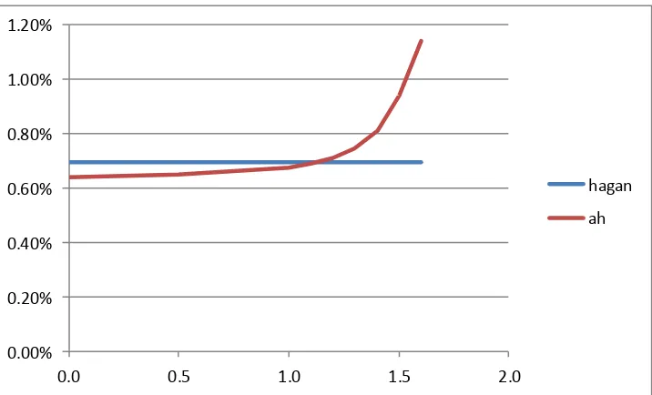
Figure 1: Implied Black volatility for our short maturity expansions in Black or normal volatility compared to Hagan’s formula. Parameters 

 

We can use (7) to retrieve the local volatility function of SABR from

 

1 1 1

( )

( )

x x y

k y k J y z k

 _  _{ }

  

Hence,

 

   

  

This result can also be found in Doust (2010) but it seems that our approach is more direct.

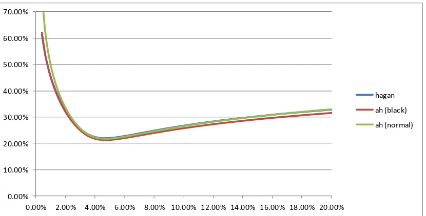
Figure 2 compares the volatility function ( )s to the local volatility function ( )k . 0.00%

10.00% 20.00% 30.00% 40.00% 50.00% 60.00% 70.00%

0.00% 2.00% 4.00% 6.00% 8.00% 10.00% 12.00% 14.00% 16.00% 18.00% 20.00%

hagan

ah (black)

Figure 2: Volatility ( )s 0.0873s0.7 compared to the local volatility ( )k J y z( ) ( )k for the case of  0.47, 0.48,T 10.

The ZABR Model

Next, we will consider the extended SABR model where the volatility process is of the CEV type 

 

Again, we will introduce an intermediate variable

 

2 1

s k

y z du

u

  



_

For which Ito expansion yields









1

2 ( )

dyz dW  ydZ O dt

Define xz1 f y

 

1

( ) (1 ) ( ) ( )

( ) [( 2) ( ) (1 ) ( )] ( )

dx z f y dy f y dZ O dt

f y dW yf y f y dZ O dt

 _{ }

  

 _

   

 

     

We conclude that the diffusion condition is satisfied if f is the solution to the ODE

0.0000% 0.5000% 1.0000% 1.5000% 2.0000% 2.5000% 3.0000% 3.5000% 4.0000% 4.5000%

0.0000% 2.0000% 4.0000% 6.0000% 8.0000% 10.0000%

 

2

2 2 2

2

2 2

1 ( ) ( ) ( ) ( ) ( ) ( ) 1 ( 2) 2 ( 2) ( ) 2 (1 ) 2(1 )( 2)

(1 ) 0 0

A y f y B y f y f y C

A y y y

B y y

C f                               

The ODE can be rearranged as

2 2 2

( ) ( ) 4 ( )( 1)

( ) ( , )

2 ( )

B y f B y f A y Cf

f y F y f

A y

   

  

which can be solved e.g. by for example Runge-Kutta. We can evaluate the solution for all strikes in one sweep by

2 1

1 1 1 1 1

( )

( ) ( , ) ( )

( ) ( ) 0

y

z k

k

x f y

z z f y z F y z x k

k k k

x k s y k s

              _{ }   _  _{ }  _{ }        (8)

Again, we can find the local volatility function as

1 1 1

( )k ( x) z ( )k f ( )y z ( ) ( ,k F y z x)

k



 _{ }   _  _{ }   

 (9)

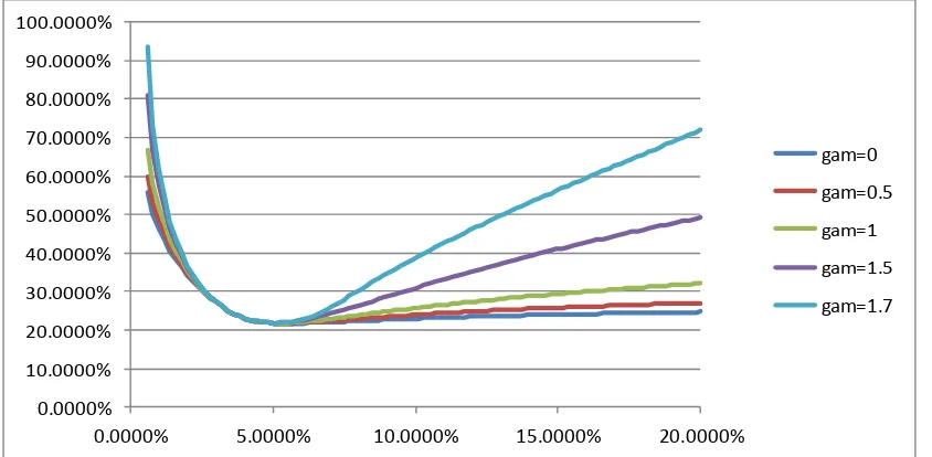
By adding  we get better control over the volatility for high strikes which in turn gives us better control over the CMS prices. This is illustrated in Figure 3.

Figure 3: Implied Black volatility smiles for different choices of . Other parameters the same as in Figure 1. 0.0000% 10.0000% 20.0000% 30.0000% 40.0000% 50.0000% 60.0000% 70.0000% 80.0000% 90.0000% 100.0000%

0.0000% 5.0000% 10.0000% 15.0000% 20.0000%

Finite Difference Volatility

Using the implied normal volatility coming from the short maturity expansion directly for pricing using (2) will not give arbitrage free option prices. In Figure 4 we have plotted the volatilities and the implied density coming from the Hagan expansion. We can see that there are negative densities and therefore arbitrages.

Figure 4: Density and implied Black Scholes volatilities from the Hagan expansion. Parameters as in figure 1.

As in Dupire (1994) we can use the local volatilities in the forward pricing PDE

2

1

( , ) ( ) ( , ) 2

(0, ) ( )

t kk

c t k k c t k

c k s k







 

(10)

The usual way of solving this is to set up a time discretisation and then use a finite difference solver. However, to gain speed we will instead use the 1 step finite difference approach introduced in Andreasen and Huge (2011). Here we need to solve the ODE

2

1

( , ) ( ) ( , ) ( )

2 kk

c t k  t k c t k  s k  (11)

In Andreasen and Huge (2011) it is shown that this approach generates a set of arbitrage free call prices for any choice of . It is also shown that the 1 step finite difference price is the Laplace transform of the solution to (10). The Laplace transform of the Gaussian distribution is the Laplace distribution

2

/ 2

2 0

1

( )

2

T s k

t T s k T v

e dt e

v

v t v t

 

   _



which is peaked at ks. Therefore if we choose   we will also get a peak in the densities.

-30 -20 -10 0 10 20 30

0 0.1 0.2 0.3 0.4 0.5 0.6 0.7 0.8

0 0.02 0.04 0.06 0.08 0.1 0.12

Instead, we will find an adjustment for the local volatility function based on the normal option pricing formula. As option prices generated by (10) and (11) should be

the same, we can substitute 2

2 / kk t

c  c  from (10) into (11) and rearrange to find









2 2

2

2 1/ 2

2 2

( , ) ( )

( ) ( )

( , )

1

( , , ( ) )

( )

, , /

( )

( ) 2(1 ) , | |

( )

( ) ( )

t

c t k s k

k k

tc t k

g t s v s k

t k

g t s v t

k x t

k P x

 





  

  





  



  

 

 

   

 

where the second (approximate) equality involves approximating the option prices by our expansion result.

We note that P x( )2 conveniently can be approximated with a 3rd or 5th order polynomial. See for example Abramowitz and Stegun (1972), (26.2.16) and (26.2.17).

The finite difference discretisation of (11) is

2

1

[1 ( ) ] ( , ) ( ) 2t k kk c t k s k



  

where kk is the second order difference operator. This equation can be represented as

a tridiagonal matrix equation on the grid { , ,k k0 1 ,kn}which in turn can be solved for { ( , )}c t ki in linear time using the tridag() algorithm in Press et al (1992). In this

matrix solution we use the expansion as boundary values at the edges of the grid:

0 0

( , ) ( , , ( ))

( , _n) ( , , ( ))_n

c t k g t s v k

c t k g t s v k

 

Figure 5: The density with and without the local volatility adjustment. Parameters as in Figure 1.

Calibrating the Volatility Function

First consider the case where we have a continuous surface of arbitrage free option prices. E.g. generated by the Andreasen and Huge (2011) interpolation scheme or from another ZABR model. Compute the local volatility function by the discrete Dupire equation

 

2 ( , ) ( )

( ) 2

, kk

c t k s k k

t c t k







  

Using (9) we can calibrate the volatility function

1

( , ) ( ) ( )

( )

F y z x k k

zP x

 _

  

where ,x y are found from (8) as the solution to the ODE.

1 1

( ) ( ) ( , )

( ) ( )

( ) ( ) 0

y z P x

k k F y z x x P x

k k

y k s x k s

  

 



 _{ }



 _{ }



   

(12)

We note that (12) can be solved for all strikes in one sweep.

However, typically, we prefer to calibrate directly to the observed discrete quotes. This is done by solving the ODE in (8) and (9) including the 1 step finite difference adjustment

-0.04 -0.03 -0.02 -0.01 0 0.01 0.02 0.03 0.04

0.0000% 2.0000% 4.0000% 6.0000% 8.0000% 10.0000%

2

1

1

( ) ( , )

( ) ( ) ( ) ( )

( , )

( ) ( ) 0

y z

k k

x F y z x

k z k

P x z k k

F y z x x k s y k s





 

  







   

 _{ }





   

(13)

Then we find the option prices using the 1 step finite difference pricer in (11). This procedure is very fast, using a non-linear solver we calibrate a non-parametric volatility function with 10 knot points to a given smile in approximately 0.001s = 1ms of CPU time. Further, as we get all option prices in one sweep, we can also include CMS forwards and option quotes in the calibration with no additional computational costs.

Though we generally use (13) in conjunction with a non-linear solver for the calibration, the direct calibration methodology (12) is relevant as it allows to directly calibrate one ZABR model to another.

Controlling the Wings

In this section we will give a few examples to illustrate how we are able to control the behaviour of the wings of the smile. Consider a model with

( )s ( )(s s s)

  

where  is a non parametric curve. s is the lower bound of the spot process. For

1

  we have absorption at s and for  1 the barrier is unattainable. In Figure 5 we fit this model to Hagan prices for  0.5,1 and s 0.02 and we see that the fit is good for positive strikes.

Figure 6: Implied Black volatilities from the ZABR model that is calibrated to the Hagan expansion for strikes in

[0.02, 0.06]. Hagan parameters as in Figure 1. 0.0000%

20.0000% 40.0000% 60.0000% 80.0000% 100.0000% 120.0000%

0.0000% 2.0000% 4.0000% 6.0000% 8.0000% 10.0000%

In Figure 7 we have plotted the resulting densities. As before the Hagan expansion produces negative densities for low positive strikes. For  0.5 we have absorption at the barrier and for  1 we see that the density below 0 is spread out.

Figure 7: Densities for Hagan and two ZABR models with  0.5,1. The ZABR models are calibrated to the Hagan expansion prices for strikes in [0.02, 0.06]. Parameters as in Figure 1.

We now use the model with  1 to illustrate the effect of . For different levels of

 we have calibrated the model to Hagan for strikes between 0.02 and 0.06. In Figure 7 we can see that all models are well calibrated. We can also see the biggest impact is for high strikes.

Figure 8: Calibration result for different choices of . All model calibrated to Hagan expansion prices for strikes in [0.02, 0.06]. Parameters as in Figure 1.

Now,  can be fixed to match CMS forwards or option quotes. In Figure 9 we have shown the impact on a CMS convexity adjustment.

-20.00 -10.00 0.00 10.00 20.00 30.00 40.00 50.00 60.00

-2.0000% 0.0000% 2.0000% 4.0000% 6.0000% 8.0000% 10.0000%

hagan

dens (beta l=0.5) dens (beta l=1)

0.0000% 20.0000% 40.0000% 60.0000% 80.0000% 100.0000% 120.0000%

0.0000% 2.0000% 4.0000% 6.0000% 8.0000%10.0000%12.0000%14.0000%16.0000%18.0000%20.0000%

hagan

ah (0)

ah (0.5)

ah (1)

ah (1.3)

Figure 9: Convexity adjustment for a CMS forward 10 x 10 for different choices of . ZABR models calibrated to Hagan expansion option prices for strikes in [0.02, 0.06].

Concluding Remarks

We have used a simple method to derive short maturity expansions for local volatilities from stochastic volatility models. The solution is an ODE which can be solved numerically for all strikes in one sweep including adjustment of the local volatility function to compensate for the 1 step finite difference option pricing. Finally, we generate use the 1 step finite difference scheme to generate option prices. The approach is very fast and it generates arbitrage free option prices. We have added flexibility to the original SABR model to get an exact fit of all quoted option prices and better control of the wings of the smile for improved CMS pricing. Also we can add CMS prices to the calibration without any extra computational costs.

0.00% 0.20% 0.40% 0.60% 0.80% 1.00% 1.20%

0.0 0.5 1.0 1.5 2.0

hagan

References

Abramowitz, M. and I. Stegun (1972): Handbook of Mathematical Functions. Dover Publications, New York.

Andersen L. and R. Ratcliffe (2002): “Extended Libor Market Models with Stochastic Volatility.” Working paper, General Re Financial Products.

Andreasen, J. and B. Huge (2011): “Volatility Interpolation.” Risk March, 86-89.

Balland, P. (2006): “Forward Smile.” ICBI Global Derivatives Presentation.

Doust, P. (2010): “No Arbitrage SABR.” Royal Bank of Scotland, working paper.

Dupire, B. (1994): “Pricing with a Smile.” Risk July, 18-20.

Hagan, Kumar, Lesniewski and Woodward (2002): “Managing Smile Risk.” Wilmott Magazine. September, 84-108.

Lewis, A. (2007): Geometries and Smile Asymptotics for a Class of Stochastic Volatility Models. UC Santa Barbara Presentation.