Article
LOGICAL ENTROPY: INTRODUCTION TO
CLASSICAL AND QUANTUM LOGICAL
INFORMATION THEORY
David Ellerman1
1 University of California Riverside; david@ellerman.org
Abstract: Logical information theory is the quantitative version of the logic of partitions just as logical probability theory is the quantitative version of the dual Boolean logic of subsets. The resulting notion of information is about distinctions, differences, and distinguishability, and is formalized using the distinctions (‘dits’) of a partition (a pair of points distinguished by the partition). All the definitions of simple, joint, conditional, and mutual entropy of Shannon information theory are derived by a uniform transformation from the corresponding definitions at the logical level. The purpose of this paper is to give the direct generalization to quantum logical information theory that similarly focuses on the pairs of eigenstates distinguished by an observable, i.e., qudits of an observable. The fundamental theorem for quantum logical entropy and measurement establishes a direct quantitative connection between the increase in quantum logical entropy due to a projective measurement and the eigenstates (cohered together in the pure superposition state being measured) that are distinguished by the measurement (decohered in the post-measurement mixed state). Both the classical and quantum versions of logical entropy have simple interpretations as "two-draw" probabilities for distinctions. The conclusion is that quantum logical entropy is the simple and natural notion of information for quantum information theory focusing on the distinguishing of quantum states.
Keywords:logical entropy; partition logic; qudits of an observable
1. Introduction
The formula for ‘classical’ logical entropy goes back to the early twentieth century [17]. It is the derivation of the formula from basic logic that is new and accounts for the name. The ordinary Boolean logic of subsets has a dual logic of partitions [12] since partitions (= equivalence relations = quotient sets) are category-theoretically dual to subsets. Just as the quantitative version of subset logic is the notion of logical finite probability, so the quantitative version of partition logic is logical information theory using the notion of logical entropy [13]. This paper generalizes that ‘classical’ (i.e., non-quantum) logical information theory to the quantum version. The classical logical information theory is briefly developed before turning to the quantum version.1
2. Duality of Subsets and Partitions
The foundations for classical and quantum logical information theory are built on the logic of partitions–which is dual (in the category-theoretic sense) to the usual Boolean logic of subsets. F. William Lawvere called a subset or, in general, a subobject a “part” and then noted: “The dual notion (obtained by reversing the arrows) of ‘part’ is the notion ofpartition.” [24, p. 85] That suggests that the Boolean logic of subsets has a dual logic of partitions ([11], [12]).
1 Applications of logical entropy have already been developed in several special mathematical settings; see [26] and the
references cited therein.
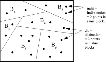
This duality can be most simply illustrated using a set function f : X → Y. The image f(X) is asubsetof the codomainYand the inverse-image or coimage2 f−1(Y)is apartitionon the domain X–where apartitionπ={B1, ...,BI}on a setUis a set of subsets or blocksBithat are mutually disjoint and jointly exhaustive (∪iBi =U). But the duality runs deeper than between subsets and partitions. The dual to the notion of an “element” (an ‘it’) of a subset is the notion of a “distinction” (a ‘dit’) of a partition, where(u,u0)∈U×Uis adistinctionorditofπif the two elements are in different blocks.
Let dit(π) ⊆ U×U be the set of distinctions orditsetofπ. Similarly an indistinctionorinditofπ
is a pair(u,u0) ∈ U×Uin the same block ofπ. Let indit(π) ⊆ U×Ube the set of indistinctions
orinditsetofπ. Then indit(π)is the equivalence relation associated withπand dit(π) =U×U−
indit(π)is the complementary binary relation that might be called apartition relationor anapartness
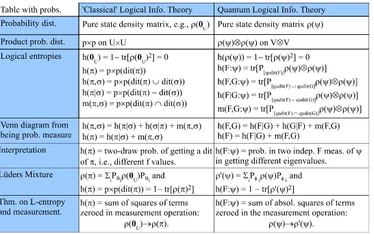
relation. The notions of a distinction and indistinction of a partition are illustrated in Figure 1.
Figure 1: Distinctions and indistinctions of a partition.
The relationships between Boolean subset logic and partition logic are summarized in Table 1 which illustrates the dual relationship between the elements (‘its’) of a subset and the distinctions (‘dits’) of a partition.
Table 1: Dual Logics: Boolean subset logic of subsets and partition logic.
3. From the logic of partitions to logical information theory
George Boole [4] developed the quantitative version of his logic of subsets by starting with the size or number of elements|S|in a subsetS ⊆U, which could then be normalized to ||US|| and given
2 In category theory, the duality between subobject-type constructions (e.g., limits) and quotient-object-type constructions
the probabilistic interpretation as the probability that a randomly drawn element fromUwould be an element ofS.
The algebra of partitionsπonUis isomorphically represented by the algebra of ditsets dit(π)⊆
U×U, so the parallel quantitative development of the logic of partitions would start with the size or number of distinctions|dit(π)|in a partitionπonU, which could then be normalized to ||dit(U×πU)||.
It has the probabilistic interpretation as the probability that two randomly drawn elements fromU (with replacement) would be a distinction ofπ.
In Gian-Carlo Rota’s Fubini Lectures [31] (and in his lectures at MIT), he remarked in view of duality between partitions and subsets that, quantitatively, the “lattice of partitions plays for information the role that the Boolean algebra of subsets plays for size or probability” [22, p. 30] or symbolically:
Logical Probability Theory Boolean Logic of Subsets =
Logical Information Theory Logic of Partitions .
Since “Probability is a measure on the Boolean algebra of events” that gives quantitatively the “intuitive idea of the size of a set”, we may ask by “analogy” for some measure to capture a property for a partition like “what size is to a set.” Rota goes on to ask:
How shall we be led to such a property? We have already an inkling of what it should be: it should be a measure of information provided by a random variable. Is there a candidate for the measure of the amount of information? [31, p. 67]
We have just seen that the parallel development suggests the normalized number of distinctions of a partition as “the measure of the amount of information”.
4. The logical theory of information
Andrei Kolmogorov has suggested that information theory should start with sets, not probabilities.
Information theory must precede probability theory, and not be based on it. By the very essence of this discipline, the foundations of information theory have a finite combinatorial character. [21, p. 39]
The notion of information-as-distinctions does start with theset of distinctions, theinformation set, of a partitionπ={B1, ...,BI}on a finite setUwhere that set of distinctions (dits) is:
dit(π) ={(u,u0):∃Bi,Bi0 ∈π,Bi6=Bi0,u∈Bi,u0∈ Bi0}.
The normalized size of a subset is the logical probability of the event, and the normalized size of the ditset of a partition is, in the sense of measure theory, “the measure of the amount of information” in a partition. Thus we define thelogical entropyof a partitionπ = {B1,...,BI}, denotedh(π), as the
size of the ditset dit(π)⊆U×Unormalized by the size ofU×U:
h(π) = ||dit(U×πU)|| = |U×U|−∑
I i=1|Bi×Bi|
|U×U| =1−∑iI=1 |B
i|
|U|
2
=1−∑I
i=1Pr(Bi)2.
In two independent draws fromU, the probability of getting a distinction of πis the probability of
not getting an indistinction.
Given any probability measurep :U →[0, 1]onU= {u1, ...,un}which definespi = p(ui)for i=1, ...,n, theproduct measure p×p:U×U→[0, 1]has for any binary relationR⊆U×Uthe value of:
p×p(R) =∑(ui,uj)∈Rp(ui)p uj
=∑(u
Thelogical entropyofπin general is the product-probability measure of its ditset dit(π)⊆U×U,
where Pr(B) =∑u∈Bp(u):
h(π) =p×p(dit(π)) =∑(u
i,uj)∈dit(π)pipj=1−∑B∈πPr(B) 2
.
There are two stages in the development of logical information. Before the introduction of any probabilities, the information set of a partitionπonUis its ditset dit(π). Then given a probability
measurep :U → [0, 1]onU, the logical entropy of the partition is just the product measure on the ditset, i.e.,h(π) =p×p(dit(π)). The standard interpretation ofh(π)is the two-draw probability of
getting a distinction of the partitionπ–just as Pr(S)is the one-draw probability of getting an element
of the subset-eventS.
5. Compound logical entropies
The compound notions of logical entropy are also developed in two stages, first as sets and then, given a probability distribution, as two-draw probabilities. After observing the similarity between the formulas holding for the compound Shannon entropies and the Venn diagram formulas that hold for any measure (in the sense of measure theory), the information theorist, Lorne L. Campbell, remarked in 1965 that the similarity:
suggests the possibility that H(α) and H(β) are measures of sets, that H(α,β) is the
measure of their union, that I(α,β)is the measure of their intersection, and thatH(α|β)
is the measure of their difference. The possibility that I(α,β) is the entropy of the
“intersection” of two partitions is particularly interesting. This “intersection,” if it existed, would presumably contain the information common to the partitionsαandβ. [6, p. 113]
Yet, there is no such interpretation of the Shannon entropies as measures of sets, but the logical entropies precisely fulfill Campbell’s suggestion (with the “intersection” of two partitions being the intersection of their ditsets). Moreover, there is a uniform requantifying transformation (see next section) that obtains all the Shannon definitions from the logical definitions and explains how the Shannon entropies can satisfy the Venn diagram formulas (e.g., as a mnemonic) while not being defined by a measure on sets.
Given partitionsπ ={B1, ...,BI}andσ=C1, ...,CJ onU, thejoint information setis the union of the ditsets which is also theditset for their joinis: dit(π)∪dit(σ) = dit(π∨σ) ⊆ U×U. Given
probabilitiesp ={p1, ...,pn}onU, thejoint logical entropyis the product probability measure on the union of ditsets:
h(π,σ) =h(π∨σ) =p×p(dit(π)∪dit(σ)) =1−∑i,jPr Bi∩Cj2.
The information set for theconditional logical entropy h(π|σ)is the difference of ditsets, and thus that
logical entropy is:
h(π|σ) =p×p(dit(π)−dit(σ)) =h(π,σ)−h(σ).
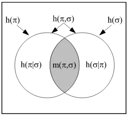
The information set for the logical mutual information m(π,σ) is the intersection of ditsets, so that
logical entropy is:
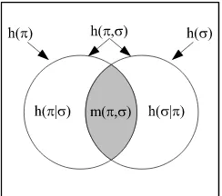
m(π,σ) =p×p(dit(π)∩dit(σ)) =h(π,σ)−h(π|σ)−h(σ|π) =h(π) +h(σ)−h(π,σ).
Figure 2: Venn diagram for logical entropies as values of a probability measurep×ponU×U. At the level of information sets (w/o probabilities), we have theinformation algebra I(π,σ)which
is the Boolean subalgebra of℘(U×U)generated by ditsets and their complements. 6. Deriving the Shannon entropies from the logical entropies
Instead of being defined as the values of a measure, the usual notions of simple and compound entropy ‘burst forth fully formed from the forehead’ of Claude Shannon [33] already satisfying the standard Venn diagram relationships.3 Since the Shannon entropies are not the values of a measure, many authors have pointed out that these Venn diagram relations for the Shannon entropies can only be taken as “analogies” or “mnemonics” ([6]; [1]). Logical information theory explains this situation since all the Shannon definitions of simple, joint, conditional, and mutual information can be obtained by a uniform requantifying transformation from the corresponding logical definitions, and the transformation preserves the Venn diagram relationships.
This transformation is possible since the logical and Shannon notions of entropy can be seen as two different ways to quantify distinctions–and thusboththeories are based on the foundational idea ofinformation-as-distinctions.
Consider the canonical case ofn equiprobable elements, pi = n1. The logical entropy of 1 = {B1, ...,Bn}whereBi ={ui}withp=
n 1 n, ...,1n
o is:
|U×U−∆| |U×U| = n
2−n
n2 =1−1n =1−Pr(Bi).
The normalized number of distinctions or ‘dit-count’ of the discrete partition1is 1−1
n =1−Pr(Bi). The general case of logical entropy for anyπ={B1, ...,BI}is the average of the dit-counts 1−Pr(Bi) for the canonical cases:
h(π) =∑iPr(Bi) (1−Pr(Bi)).
In the canonical case of 2n equiprobable elements, the minimum number of binary partitions (“yes-or-no questions” or “bits”) whose join is the discrete partition1 = {B1, ...,B2n}with Pr(Bi) =
1
2n, i.e., that it takes to uniquelyencodeeach distinct element, isn, so the Shannon-Hartley entropy [18] is the canonical bit-count:
n=log2(2n) =log21/21n
=log2Pr(1B i)
.
The general case Shannon entropy is the average of these canonical bit-counts log2Pr(1B i)
:
H(π) =∑iPr(Bi)log2
1 Pr(Bi)
.
TheDit-Bit Transform essentially replaces the canonical dit-counts by the canonical bit-counts. First express any logical entropy concept (simple, joint, conditional, or mutual) as an average of canonical dit-counts 1−Pr(Bi), and then substitute the canonical bit-count log
1 Pr(Bi)
to obtain the corresponding formula as defined by Shannon. Table 2 gives examples of the dit-bit transform.
Table 2: Summary of the dit-bit transform
For instance,
h(π|σ) =h(π,σ)−h(σ) =∑i,jPr Bi∩Cj 1−Pr Bi∩Cj−∑jPr Cj 1−Pr Cj is the expression forh(π|σ)as an average over 1−Pr Bi∩Cjand 1−Pr Cj, so applying the dit-bit transform gives:
∑i,jPr Bi∩Cj
log 1/ Pr Bi∩Cj
−∑jPr Cj
log 1/ Pr Cj
=H(π,σ)−H(σ) =H(π|σ).
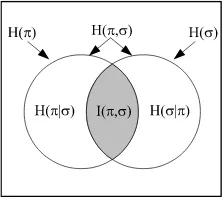
The dit-bit transform is linear in the sense of preserving plus and minus, so the Venn diagram formulas, e.g.,h(π,σ) =h(σ) +h(π|σ), which are automatically satisfied by logical entropy since it
is a measure, carry over to Shannon entropy, e.g.,H(π,σ) = H(σ) +H(π|σ)as in Figure 3, in spite
of it not being a measure (in the sense of measure theory):
Figure 3: Venn diagram mnemonic for Shannon entropies
7. Shannon information theory for coding and communications
All the compound definitions of the Shannon information theory can be derived from the logical definitions which are a product probability measure on the sets generated by the set operations on ditsets (e.g., union, difference, and intersection). Hence the question of the relation between the two theories naturally arises. The claim here is that the logical theory is the foundational theory that explains what information is at the logical level (information as distinctions) while the Shannon theory is a specialized theory for the purposes of coding and communications theory [33]. In spite of its great success in these fields, the specialized and non-foundational nature of the Shannon theory is emphasized by the way its definitions can breakdown when extended in a number of ways while the logical definitions are stable in all the same cases (see Table 3).
e.g., [8, p. 48] or [38, p. 30]. But for a countably infinite probability distribution p = (p1,p2, ...), we have∑ipi = 1 soh(p) = 1−∑ip2i is perfectly well-defined. In the process of moving from a discrete distributionpto a continuous distribution f(x), the term log∆1x
i
blows up [27, pp. 34-38] as the mesh size∆xi →0 so the continuous definitionH(f) = −R f(x)log(f(x))dxis chosen by analogy and "is not in any sense a measure of the randomness ofX" [27, p. 38] in addition to possibly having negative values [37, p. 74]. But for a continuous distributionR
f(x)dx = 1, so the logical entropyh(f) =1−R
f(x)2dxis always well-defined. Perhaps the most surprising case is that the conventional mutual informationI(X,Y,Z)for three or more random variables can be negative and thus uninterpretable as is noted in many texts, e.g., [1, pp. 128-131], [15, p. 58], [9, p. 52-3], [8, p. 49], and [38, pp.103-4]. In contrast, all the logical entropy notions for any number of random variables have two-draw probability interpretations and thus take values in the half-open interval[0, 1).
Table 3: Comparisons of generalizations of Shannon and logical entropy
Finally, although not directly related to the comparison with logical entropy, it might be noted that much has been written over the years as if Shannon entropy had the same functional form as Boltzmann’s entropy formula lnn n!
1!...nm!
in statistical mechanics–even to the point of using phrases like “Shannon-Boltzmann entropy.” But the Shannon entropy is obtained as a numerical approximation by using the first two terms in one form of the Stirling series:
ln(n!) =
Shannon
z }| {
nln(n)−n+12ln(2πn) +(12)1n −(360)1n3 +(1260)1 n5 − (1680)1 n7 +....
By using more terms, one gets an infinite series ofbetter and betterapproximations to the Boltzmann entropy formula in statistical mechanics (see [25, p. 2] for a similar point).
8. Logical entropy via density matrices
The transition to quantum logical entropy is facilitated by reformulating the classical logical theory in terms of density matrices. Let U = {u1, ...,un} be the sample space with the point probabilitiesp= (p1, ...,pn). An eventS⊆Uhas the probability Pr(S) =∑uj∈Spj.
For any eventSwith Pr(S)>0, let |Si= √1
Pr(S)(χS(u1) √
p1, ...,χS(un)√pn)t
(the superscripttindicates transpose) which is a normalized column vector inRn whereχS : U → {0, 1}is the characteristic function forS, and lethS| be the corresponding row vector. Since |Siis normalized,hS|Si= 1. Then thedensity matrixrepresenting the eventSis then×nsymmetric real matrix:
ρ(S) =|Si hS|so that(ρ(S))j,k=
( 1
Pr(S) √
pjpkforuj,uk∈S
Thenρ(S)2=|Si hS|Si hS|=ρ(S)so borrowing language from quantum mechanics,ρ(S)is said to
be apure statedensity matrix.
Given any partitionπ= {B1, ...,BI}onU, its density matrix is the average of the block density matrices:
ρ(π) =∑iPr(Bi)ρ(Bi).
Then ρ(π) represents the mixed state, experiment, or lottery where the event Bi occurs with probability Pr(Bi). A little calculation connects the logical entropy h(π) of a partition with the
density matrix treatment:
h(π) =1−∑iI=1Pr(Bi)2=1−tr h
ρ(π)2
i
=h(ρ(π))
whereρ(π)2is substituted for Pr(Bi)2and the trace is substituted for the summation.
For the throw of a fair die,U = {u1,u3,u5,u2,u4,u6}(note the odd faces ordered before the even faces in the matrix rows and columns) whereujrepresents the numberjcoming up, the density matrixρ(0)is the “pure state” 6×6 matrix with each entry being 16.
ρ(0) =
1/6 1/6 1/6 1/6 1/6 1/6 1/6 1/6 1/6 1/6 1/6 1/6 1/6 1/6 1/6 1/6 1/6 1/6 1/6 1/6 1/6 1/6 1/6 1/6 1/6 1/6 1/6 1/6 1/6 1/6 1/6 1/6 1/6 1/6 1/6 1/6 u1 u3 u5 u2 u4 u6 .
The nonzero off-diagonal entries represent indistinctions or indits of the partition 0, or in quantum terms, “coherences,” where all 6 “eigenstates” cohere together in a pure “superposition” state. All pure states have logical entropy of zero, i.e.,h(0) = 0 (i.e., no dits) since tr[ρ] =1 for any
density matrix so ifρ(0)2=ρ(0), then tr
h
ρ(0)2
i
=tr[ρ(0)] =1 andh(0) =1−tr
h
ρ(0)2
i =0. The logical operation ofclassifyingundistinguished entities (like the six faces of the die before a throw to determine a face up) by a numerical attribute makes distinctions between the entities with different numerical values of the attribute. Classification (also called sorting, fibering, or partitioning [23, Section 6.1]) is the classical operation corresponding to the quantum operation of ‘measurement’ of a superposition state by an observable to obtain a mixed state.
Now classify or “measure” the die-faces by the parity-of-the-face-up (odd or even) partition (observable) π = {Bodd,Beven} = {{u1,u3,u5},{u2,u4,u6}}. Mathematically, this is done by the Lüders mixture operation [2, p. 279], i.e., pre- and post-multiplying the density matrixρ(0)byPodd and byPeven, the projection matrices to the odd or even components, and summing the results:
Poddρ(0)Podd+Pevenρ(0)Peven
=
1/6 1/6 1/6 0 0 0
1/6 1/6 1/6 0 0 0
1/6 1/6 1/6 0 0 0
0 0 0 0 0 0
0 0 0 0 0 0
0 0 0 0 0 0
+
0 0 0 0 0 0
0 0 0 0 0 0
0 0 0 0 0 0
0 0 0 1/6 1/6 1/6
0 0 0 1/6 1/6 1/6
0 0 0 1/6 1/6 1/6
=
1/6 1/6 1/6 0 0 0
1/6 1/6 1/6 0 0 0
1/6 1/6 1/6 0 0 0
0 0 0 1/6 1/6 1/6
0 0 0 1/6 1/6 1/6
0 0 0 1/6 1/6 1/6
Theorem 1 (Fundamental (Classical)). The increase in logical entropy, h(ρ(π))−h(ρ(0)), due to a
Lüders mixture operation is the sum of amplitudes squared of the non-zero off-diagonal entries of the beginning density matrix that are zeroed in the final density matrix.
Proof. Since for any density matrixρ, trρ2= ∑i,jρij 2
[16, p. 77], we have:h(ρ(π))−h(ρ(0)) =
1−trhρ(π)2
i
−1−trhρ(0)2
i
= trhρ(0)2
i
−trhρ(π)2
i
= ∑i,j ρij(0)
2
− ρij(π)
2 . If (ui,ui0) ∈ dit(π), then and only then are the off-diagonal terms corresponding toui andui0zeroed by the Lüders operation.
The classical fundamental theorem connects the concept of information-as-distinctions to the process of ‘measurement’ or classification which uses some attribute (like parity in the example) or ‘observable’ to make distinctions.
In the comparison with the matrix ρ(0) of all entries 16, the entries that got zeroed in the
Lüders operation ρ(0) −→ ρ(π) correspond to the distinctions created in the transition 0 =
{{u1, ...,u6}} −→ π = {{u1,u3,u5},{u2,u4,u6}}, i.e., the odd-numbered faces were distinguished from the even-numbered faces by the parity attribute. The increase in logical entropy = sum of the
squares of the off-diagonal elements that were zeroed =h(π)−h(0) =2×9×
1 6
2
= 1836 = 12. The
usual calculations of the two logical entropies are:h(π) =2×
1 2
2
= 12andh(0) =1−1=0. Since, in quantum mechanics, a projective measurement’s effect on a density matrixisthe Lüders mixture operation, that means that the effects of the measurement are the above-described “making distinctions” by decohering or zeroing certain coherence terms in the density matrix, and the sum of the absolute squares of the coherences that were decohered is the increase in the logical entropy.
9. Quantum Logical Information Theory: Commuting Observables
The idea of information-as-distinctions carries over to quantum mechanics.
[Information] is the notion of distinguishability abstracted away from what we are distinguishing, or from the carrier of information. ...And we ought to develop a theory of information which generalizes the theory of distinguishability to include these quantum properties... . [3, p. 155]
Let F : V → V be a self-adjoint operator (observable) on a n-dimensional Hilbert space V with the real eigenvalues φ1, ...,φI and let U = {u1, ...,un} be an orthonormal (ON) basis of eigenvectors ofF. The quantum version of a dit, aqudit, is a pair of states definitely distinguishable bysome observable4–which is analogous classically to a pair(u,u0) of distinct elements of U that are distinguishable by some partition (i.e.,1). In general, aquditisrelativized to an observable–just as classically a distinction is a distinctionof a partition. Then there is a set partitionπ = {Bi}i=1,...,Ion the ON basisUso thatBiis a basis for the eigenspace of the eigenvalueφiand|Bi|is the "multiplicity" (dimension of the eigenspace) of the eigenvalueφi fori =1, ...,I. Note that the real-valued function f : U → Rthat takes each eigenvector in uj ∈ Bi ⊆ Uto its eigenvalue φi so that f−1(φi) = Bi contains all the information in the self-adjoint operatorF : V →V sinceFcan be reconstructed by defining it on the basisUasFuj = f ujuj.
The generalization of ‘classical’ logical entropy to quantum logical entropy is straightforward using the usual ways that set-concepts generalize to vector-space concepts: subsets→subspaces, set partitions→direct-sum decompositions of subspaces5, Cartesian products of sets→tensor products
4 Any nondegenerate self-adjoint operator such as∑n
k=1kP[uk], whereP[uk]is the projection to the one-dimensional subspace generated byuk, will distinguish all the vectors in the orthonormal basisU.
5 Hence the ‘classical’ logic of partitions on a set will generalize to the quantum logic of direct-sum decompositions [14] that
of vector spaces, and ordered pairs (uk,uk0) ∈ U×U →basis elements uk⊗uk0 ∈ V⊗V. The eigenvalue function f : U → R determines a partition
f−1(φi) i∈I on Uand the blocks in that partition generate the eigenspaces ofFwhich form a direct-sum decomposition ofV.
Classically, adit of the partition
f−1(φi) i∈I onUis a pair(uk,uk0)of points in distinct blocks of the partition, i.e., f(uk) 6= f(uk0). Hence aqudit of Fis a pair(uk,uk0)(interpreted asuk⊗uk0 in the context ofV⊗V) of vectors in the eigenbasis definitely distinguishable byF, i.e., f(uk)6= f(uk0), distinctF-eigenvalues. LetG :V →Vbe another self-adjoint operator onVwhich commutes with Fso that we may then assume thatUis an orthonormal basis of simultaneous eigenvectors ofFand G. Let
γj j∈Jbe the set of eigenvalues ofGand letg:U →Rbe the eigenvalue function so a pair
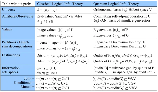
(uk,uk0)is aqudit of Gifg(uk)6=g(uk0), i.e., if the two eigenvectors have distinct eigenvalues ofG. As in classical logical information theory, information is represented by certain subsets–or, in the quantum case, subspaces–prior to the introduction of any probabilities. Since the transition from classical to quantum logical information theory is straightforward, it will be presented in table form in Table 5 (which does not involve any probabilities)–where the qudits (uk,uk0)are interpreted as uk⊗uk0.
Table 5: The parallel development of classical and quantum logical information prior to probabilities.
The information subspace associated with F is the subspace [qudit(F)] ⊆ V⊗V generated by the qudits uk⊗uk0 of F. If F = λI is a scalar multiple of the identity I, then it has no qudits so its
information space[qudit(λI)]is the zero subspace. It is an easy implication of the Common Dits
Theorem of classical logical information theory ([10, Proposition 1] or [11, Theorem 1.4]) that any two nonzero information spaces[qudit(F)]and[qudit(G)]have a nonzero intersection, i.e., have a nonzero mutual information space. That is, there are always two eigenvectorsuk anduk0 that have different eigenvalues both byFand byG.
In a measurement, the observables do not provide the point probabilities; they come from the pure (normalized) stateψbeing measured. Let|ψi=∑jn=1uj|ψ uj
=∑nj=1αj uj
be the resolution of|ψiin terms of the orthonormal basisU = {u1, ...,un}of simultaneous eigenvectors forFandG. Thenpj=αjα∗j (α∗j is the complex conjugate ofαj) forj=1, ...,nare the point probabilities onUand the pure state density matrixρ(ψ) = |ψi hψ|(wherehψ| = |ψi†is the conjugate-transpose) has the
entries: ρjk(ψ) = αjα∗k so the diagonal entriesρjj(ψ) = αjα∗j = pjare the point probabilities. Table 6 gives the remaining parallel development with the probabilities provided by the pure stateψwhere
Table 6: The parallel development of classical and quantum logical entropies for commutingFand G.
The formulah(ρ) =1−trρ2is hardly new. Indeed, trρ2is usually called thepurityof the
density matrix since a stateρispureif and only if trρ2 =1 soh(ρ) =0, and otherwise trρ2 <1
soh(ρ)> 0 and the state is said to bemixed. Hence the complement 1−trρ2has been called the
“mixedness” [20, p. 5] or “impurity” of the stateρ.6 What is new is not the formula but the whole
backstory of partition logic outlined above which gives the logical notion of entropy arising out of partition logic as the normalized counting measure on ditsets–just as logical probability arises out of Boolean subset logic as the normalized counting measure on subsets. The basic idea of information is differences, distinguishability, and distinctions ([10], [13]), so the logical notion of entropy is the measure of the distinctions or dits of a partition and the corresponding quantum version is the measure of the qudits of an observable.
The classical dit-bit transform connecting the logical theory to the Shannon theory also carries over to the quantum version. Writing the quantum logical entropy of a density matrixρ ash(ρ) =
tr[ρ(1−ρ)], the quantum version of the dit-bit transform(1−ρ)−→ −log(ρ)yields the usual Von
Neumann entropyS(ρ) = −tr[ρlog(ρ)][28, p. 510]. The fundamental theorem connecting logical
entropy and the operation of classification-measurement also carries over to the quantum case.
10. Two Theorems about quantum logical entropy
Classically, a pair of elements uj,uk
either ‘cohere’ together in the same block of a partition onU, i.e., are an indistinction of the partition, or they don’t, i.e., are a distinction of the partition. In the quantum case, the nonzero off-diagonal entriesαjα∗k in the pure state density matrixρ(ψ) =
|ψi hψ|are called quantum “coherences” ([7, p. 303]; [2, p.177]) because they give the amplitude of
the eigenstates uj
and |uki“cohering” together in the coherent superposition state vector|ψi =
∑n j=1
uj|ψ uj
= ∑jαj uj
. The coherences are classically modelled by the nonzero off-diagonal entries√pjpkfor the indistinctions uj,uk∈Bi×Bi, i.e., coherences≈indistinctions.
For an observable F, let φ : U → R be for F-eigenvalue function assigning the eigenvalue
φ(ui) = φi for each ui in the ON basis U = {u1, ...,un} of F-eigenvectors. The range of φis the
set of F-eigenvalues {φ1, ...,φI}. Let Pφi : V → V be the projection matrix in the U-basis to the eigenspace ofφi. The projectiveF-measurement of the stateψtransforms the pure state density matrix ρ(ψ)(represented in the ON basisUofF-eigenvectors) to yield the Lüders mixture density matrix ρ0(ψ) = ∑iI=1Pφiρ(ψ)Pφi [2, p. 279]. The off-diagonal elements of ρ(ψ)that are zeroed in ρ
0(
ψ)
6 It is also called by the misnomer “linear entropy” [5] even though it is obviously quadratic inρ–so we will not continue
are the coherences (quantum indistinctions orquindits) that are turned into ‘decoherences’ (quantum distinctions or qudits of the observable being measured).
For any observableFand a pure stateψ, a quantum logical entropy was defined ash(F:ψ) =
trhP[qudit(F)]ρ(ψ)⊗ρ(ψ)
i
. That definition was the quantum generalization of the ‘classical’ logical entropy defined as h(π) = p×p(dit(π)). When a projective F-measurement is performed on ψ, the pure state density matrix ρ(ψ) is transformed into the mixed state density matrix by the
quantum Lüders mixture operation which then defines the quantum logical entropyh(ρ0(ψ)) =1−
trhρ0(ψ)2
i
. The first test of how the quantum logical entropy notions fit together is showing that these two entropies are the same:h(F:ψ) =h(ρ0(ψ)). The proof shows that they are both equal to classical
logical entropy of the partitionπ(F:ψ)defined on the ON basisU = {u1, ...,un}ofF-eigenvectors by theF-eigenvalues with the point probabiltiespj =α∗jαj. That is, the inverse-imagesBi =φ−1(φi) of the eigenvalue functionφ : U → R define the eigenvalue partition π(F:ψ) = {B1, ...,BI}on the ON basisU = {u1, ...,un}with the point probabilities pj = α∗jαj provided by the state |ψifor
j = 1, ...,n. The classical logical entropy of that partition is: h(π(F:ψ)) = 1−∑iI=1p(Bi)2where p(Bi) =∑uj∈Bipj.
We first show that h(F:ψ) = tr
h
P[qudit(F)]ρ(ψ)⊗ρ(ψ) i
= h(π(F:ψ)). Now qudit(F) =
uj⊗uk :φ uj6=φ(uk) and[qudit(F)]is the subspace ofV⊗Vgenerated by it. Then×npure state density matrix ρ(ψ) has the entries ρjk(ψ) = αjα∗k, andρ(ψ)⊗ρ(ψ) is an n2×n2 matrix.
The projection matrix P[qudit(F)] is an n2×n2 diagonal matrix with the diagonal entries, indexed by j,k = 1, ...,n: hP[qudit(F)]
i
jjkk = 1 if φ uj
6
= φ(uk) and 0 otherwise. Thus in the product
P[qudit(F)]ρ(ψ)⊗ρ(ψ), the nonzero diagonal elements are thepjpkwhereφ uj
6
= φ(uk)and so the trace is∑nj.k=1
pjpk :φ uj6=φ(uk) which, by definition, ish(F:ψ). Since∑nj=1pj =∑iI=1p(Bi) = 1,∑Ii=1p(Bi)
2
=1=∑Ii=1p(Bi)2+∑i6=i0p(Bi)p(Bi0). By grouping thepjpkin the trace according to the blocks ofπ(F:ψ), we have:
h(F:ψ) =tr
h
P[qudit(F)]ρ(ψ)⊗ρ(ψ)
i
=∑nj.k=1
pjpk :φ uj6=φ(uk) =∑i6=i0∑pjpk:uj∈Bi,uk∈Bi0 =∑i6=i0p(Bi)p(Bi0)
=1−∑I
i=1p(Bi)2=h(π(F:ψ)).
To show thath(ρ0(ψ)) =1−tr
h
ρ0(ψ)2
i
=h(π(F:ψ))forρ0(ψ) =∑Ii=1Pφiρ(ψ)Pφi, we need to compute trhρ0(ψ)2
i
. An off-diagonal element inρjk(ψ) =αjα∗k ofρ(ψ)survives (i.e., is not zeroed
and has the same value) the Lüders operation if and only ifφ uj = φ(uk). Hence thejthdiagonal element ofρ0(ψ)2is
∑n k=1
n
α∗jαkαjα∗k :φ uj
=φ(uk) o
=∑nk=1
pjpk:φ uj
=φ(uk) = pjp(Bi)
whereuj ∈ Bi. Then grouping thejthdiagonal elements foruj ∈ Bigives∑uj∈Bi pjp(Bi) = p(Bi) 2.
Hence the whole trace is: trhρ0(ψ)2
i
=∑iI=1p(Bi)2and thus:
h(ρ0(ψ)) =1−tr
h
ρ0(ψ)2
i
=1−∑I
i=1p(Bi)2=h(F:ψ).
This completes the proof of the following theorem.
Theorem 2. h(F:ψ) =h(π(F:ψ)) =h(ρ0(ψ)).
classifying the faces of a die by their parity. The fundamental theorem about quantum logical entropy and projective measurement shows how the quantum logical entropy created (starting with h(ρ(ψ)) =0 for the pure stateψ) by the measurement can be computed directly from the coherences
ofρ(ψ)that are decohered inρ0(ψ).
Theorem 3(Fundamental (Quantum)). The increase in quantum logical entropy, h(F:ψ) = h(ρ0(ψ)),
due to the F-measurement of the pure stateψis the sum of the absolute squares of the nonzero off-diagonal
terms [coherences] inρ(ψ)(represented in an ON basis of F-eigenvectors) that are zeroed [‘decohered’] in the
post-measurement Lüders mixture density matrixρ0(ψ) =∑iI=1Pφiρ(ψ)Pφi.
Proof. h(ρ0(ψ))−h(ρ(ψ)) =
1−trhρ0(ψ)2
i
−1−trhρ(ψ)2
i =∑jk
ρjk(ψ)
2
− ρ
0
jk(ψ)
2 .
Ifujandukare a qudit ofF, then and only then are the corresponding off-diagonal terms zeroed by the Lüders mixture operation∑I
i=1Pφiρ(ψ)Pφi to obtainρ
0(
ψ)fromρ(ψ).
Density matrices have long been a standard part of the machinery of quantum mechanics. The Fundamental Theorem for logical entropy and measurement shows there is a simple, direct, and quantitative connection between density matrices and logical entropy. The Theorem directly connects the changes in the density matrix due to a measurement (sum of absolute squares of zeroed off-diagonal terms) with the increase in logical entropy due to theF-measurementh(F:ψ) =
trhP[qudit(F)]ρ(ψ)⊗ρ(ψ) i
=h(ρ0(ψ))(whereh(ρ(ψ)) =0 for the pure stateψ).
This direct quantitative connection between state discrimination and quantum logical entropy reinforces the judgment of Boaz Tamir and Eli Cohen ([34], [35]) that quantum logical entropy is a natural and informative entropy concept for quantum mechanics.
We find this framework of partitions and distinction most suitable (at least conceptually) for describing the problems of quantum state discrimination, quantum cryptography and in general, for discussing quantum channel capacity. In these problems, we are basically interested in a distance measure between such sets of states, and this is exactly the kind of knowledge provided by logical entropy [Reference to [10]]. [34, p. 1]
Moreover, the quantum logical entropy has a simple “two-draw probability” interpretation, i.e., h(F:ψ) =h(ρ0(ψ))is the probability that two independentF-measurements ofψwill yield distinct
F-eigenvalues, i.e., will yield a qudit ofF. In contrast, the Von Neumann entropy has no such simple interpretation and there seems to be no such intuitive connection between pre- and post-measurement density matrices and Von Neumann entropy–although Von Neumann entropy also increases in a projective measurement [28, Theorem 11.9, p. 515].
11. Quantum Logical Information Theory: Non-commuting Observables
11.1. Classical logical information theory with two sets X and Y
The usual (‘classical’) logical information theory for a probability distribution{p(x,y)}onX×Y (finite) in effect uses the discrete partition onXandY[13]. For the general case of quantum logical entropy for not-necessarily commuting observables, we need to first briefly develop the classical case with general partitions onXandY.
Given two finite setsXand Yand real-valued functions f : X → R with values{φi}iI=1 and
g:Y→Rwith values
γj J
j=1, each function induces a partition on its domain:
π=f−1(φi) i∈I ={B1, ...,BI}onX, andσ=
g−1 γ
j j∈J =
C1, ...,CJ onY.
A partitionπ = {B1, ...,BI}onXand a partitionσ =C1, ...,CJ onYdefine aproduct partition
π×σ on X×Y whose blocks areBi×Cj i,j. Then π inducesπ×0Y onX×Y (where0Y is the indiscrete partition onY) andσinduces0X×σonX×Y. The corresponding ditsets or information
sets are:
• dit(π×0Y) ={((x,y),(x0,y0)): f(x)6= f(x0)} ⊆(X×Y)2; • dit(0X×σ) ={((x,y),(x0,y0)):g(y)6=g(y0)} ⊆(X×Y)2;
• dit(π×σ) =dit(π×0Y)∪dit(0X×σ); and so forth.
Given a joint probability distributionp :X×Y →[0, 1], the product probability distribution is p×p:(X×Y)2→[0, 1].
All the logical entropies are just the product probabilities of the ditsets and their union, differences, and intersection:
• h(π×0Y) =p×p(dit(π×0Y)); • h(0X×σ) =p×p(dit(0X×σ));
• h(π×σ) =p×p(dit(π×σ)) = p×p(dit(π×0Y)∪dit(0X×σ));
• h(π×0Y|0X×σ) =p×p(dit(π×0Y)−dit(0X×σ));
• h(0X×σ|π×0Y) =p×p(dit(0X×σ)−dit(π×0Y)); • m(π×0Y,0X×σ) =p×p(dit(π×0Y)∩dit(0X×σ)).
All the logical entropies have the usual two-draw probability interpretation where the two independent draws fromX×Yare(x,y)and(x0,y0)and can be interpreted in terms of the f-values andg-values:
• h(π×0Y)= probability of getting distinct f-values; • h(0X×σ)= probability of getting distinctg-values;
• h(π×σ)= probability of getting distinct f orgvalues;
• h(π×0Y|0X×σ)= probability of getting distinct f-values but sameg-values;
• h(0X×σ|π×0Y)= probability of getting distinctg-values but samef-values; • m(π×0Y,0X×σ)= probability of getting distinctf and distinctgvalues.
We have defined all the logical entropies by the general method of the product probabilities on the ditsets. In the first three cases, h(π×0Y),h(0X×σ), and h(π×σ), they were the logical
entropies of partitions onX×Yso they could equivalently be defined using density matrices. The case ofh(π×σ)illustrates the general case. Ifρ(π)is the density matrix defined forπonXandρ(σ)
the density matrix forσonY, thenρ(π×σ) = ρ(π)⊗ρ(σ)is the density matrix forπ×σdefined
onX×Y, and:
h(π×σ) =1−tr
h
ρ(π×σ)2
i .
The marginal distributions are: pX(x) = ∑yp(x,y) and pY(y) = ∑xp(x,y). Since π is a partition onX, there is also the usual logical entropyh(π) = pX×pX(dit(π)) = 1−tr
h
ρ(π)2
i = h(π×0Y)where dit(π)⊆X×Xand similarly forpY.
Since the context should be clear, we may henceforth adopt the old notation from the case where
π andσ were partitions on the same setU, i.e.,h(π) = h(π×0Y),h(σ) = h(0X×σ),h(π,σ) =
h(π×σ), etc.
Figure 4: Venn diagram for logical entropies as values of a probability measurep×pon(X×Y)2. The previous treatment ofh(X),h(Y),h(X,Y),h(X|Y),h(Y|X), andm(X,Y)in [13] was just the special cases whereπ=1Xandσ=1Y.
11.2. Quantum logical entropies with non-commuting observables
As before in the case of commuting observables, the quantum case can be developed in close analogy with the previous classical case. Given a finite-dimensional Hilbert space V and not necessarily commuting observables F,G : V → V, let X be an orthonormal basis of V of F-eigenvectors and letYbe an orthonormal basis forVofG-eigenvectors (so|X|=|Y|).
Let f : X →Rbe the eigenvalue function forFwith values{φi}iI=1, and letg : Y → Rbe the eigenvalue function forGwith values
γj J j=1.
Each eigenvalue function induces a partition on its domain:
π=f−1(φi) ={B1, ...,BI}onX, andσ=g−1 γj =C1, ...,CJ onY.
We associated with the ordered pair(x,y), the basis elementx⊗yin the basis{x⊗y}x∈X,y∈Yfor V⊗V. Then each pair of pairs((x,y),(x0,y0))is associated with the basis element(x⊗y)⊗(x0⊗y0) in(V⊗V)⊗(V⊗V) = (V⊗V)2.
Instead of ditsets or information sets, we now have qudit subspaces or information subspaces. ForR⊆(V⊗V)2, let[R]be the subspace generated byR. We simplify notation ofqudit(π×0Y) = qudit(π) ={(x⊗y)⊗(x0⊗y0): f(x)6= f(x0)}, etc.
• [qudit(π)] = [{(x⊗y)⊗(x0⊗y0): f(x)6= f(x0)}];
• [qudit(σ)] = [{(x⊗y)⊗(x0⊗y0):g(y)6=g(y0)}];
• [qudit(π,σ)] = [qudit(π)∪qudit(σ)], and so forth.7
A normalized state|ψionV⊗Vdefines a pure state density matrixρ(ψ) = |ψi hψ|. Letαx,y = hx⊗y|ψi so if P[x⊗y] is the projection to the subspace (ray) generated by x⊗y in V⊗V, then a probability distribution onX×Yis defined by:
p(x,y) =αx,yα∗x,y=tr
h
P[x⊗y]ρ(ψ) i
,
or more generally, for a subspaceT ⊆V⊗V, a probability distribution is defined on the subspaces by:
Pr(T) =tr[PTρ(ψ)].
Then the product probability distribution p×p on the subspaces of (V⊗V)2 defines the quantum logical entropies when applied to the information subspaces:
7 It is again an easy implication of the aforementioned Common Dits Theorem that any two nonzero information spaces
• h(F:ψ) =p×p([qudit(π)]) =tr
h
P[qudit(π)](ρ(ψ)⊗ρ(ψ)) i
;
• h(G:ψ) =p×p([qudit(σ)]) =tr
h
P[qudit(σ)](ρ(ψ)⊗ρ(ψ))
i ;
• h(F,G:ψ) =p×p([qudit(π)∪qudit(σ)]) =tr
h
P[qudit(π)∪qudit(σ)](ρ(ψ)⊗ρ(ψ)) i
;
• h(F|G:ψ) =p×p([qudit(π)−qudit(σ)]) =tr
h
P[qudit(π)−qudit(σ)](ρ(ψ)⊗ρ(ψ))
i ;
• h(G|F:ψ) =p×p([qudit(σ)−qudit(π)]) =tr
h
P[qudit(σ)−qudit(π)](ρ(ψ)⊗ρ(ψ)) i
;
• m(F,G:ψ) =p×p([qudit(π)∩qudit(σ)]) =tr
h
P[qudit(π)∩qudit(σ)](ρ(ψ)⊗ρ(ψ))
i .
The observableF :V →Vdefines an observableF⊗I :V⊗V→V⊗Vwith the eigenvectors x⊗v for any nonzerov ∈ V and with the same eigenvaluesφ1, ...,φI.8 Then in two independent
measurements ofψby the observableF⊗I, we have:
h(F:ψ)= probability of getting distinct eigenvaluesφiandφi0, i.e., of getting a qudit ofF. In a similar manner, G : V → V defines the observable I⊗G : V⊗V → V⊗V with the eigenvectorsv⊗yand with the same eigenvaluesγ1, ...,γJ. Then in two independent measurements
ofψby the observableI⊗G, we have:
h(G:ψ)= probability of getting distinct eigenvaluesγjandγj0.
The two observables F,G : V → V define an observable F⊗G : V⊗V → V⊗V with the eigenvectors x⊗y for(x,y) ∈ X×Y and eigenvalues f(x)g(y) = φiγj. To cleanly interpret the
compound logical entropies, we assume there is no accidental degeneracy so there are noφiγj =φi0γj0 fori6=i0andj=6 j0. Then for two independent measurements ofψbyF⊗G, the compound quantum
logical entropies can be interpreted as the following “two-measurement” probabilities:
• h(F,G:ψ)= probability of getting distinct eigenvaluesφiγj 6=φi0γj0wherei6=i0orj6=j0; • h(F|G:ψ)= probability of getting distinct eigenvaluesφiγj6=φi0γjwherei6=i0;
• h(G|F:ψ)= probability of getting distinct eigenvaluesφiγj6=φiγj0wherej6=j0;
• m(F,G:ψ)= probability of getting distinct eigenvaluesφiγj 6=φi0γj0wherei6=i0andj6=j0. All the quantum logical entropies have been defined by the general method using the information subspaces, but in the first three casesh(F:ψ), h(G:ψ), and h(F,G:ψ), the density
matrix method of defining logical entropies could also be used. Then the fundamental theorem could be applied relating the quantum logical entropies to the zeroed entities in the density matrices indicating the eigenstates distinguished by the measurements.
The previous set identities for disjoint unions now become subspace identities for direct sums such as:
[qudit(π)∪qudit(σ)] = [qudit(π)−qudit(σ)]⊕[qudit(π)∩qudit(σ)]⊕[qudit(σ)−qudit(π)].
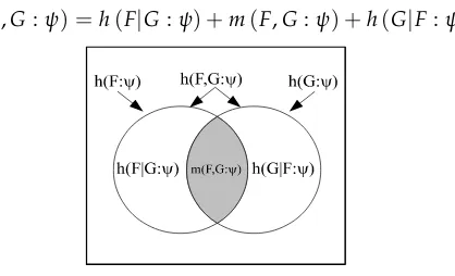
Hence the probabilities are additive on those subspaces as shown in Figure 5:
h(F,G:ψ) =h(F|G:ψ) +m(F,G:ψ) +h(G|F:ψ).
Figure 5: Venn diagram for quantum logical entropies as probabilities on(V⊗V)2.
11.3. Quantum logical entropies of density operators in general
The extension of the classical logical entropyh(p) = 1−∑n
i=1p2i of a probability distribution p = (p1, ...,pn) to the quantum case is h(ρ) = 1−trρ2 where a density matrix ρ replaces the
probability distribution p and the trace replaces the summation. In the previous section, quantum logical entropies were defined in terms of given observablesF,G:V→V(as self-adjoint operators) as well as a stateψand its density matrixρ(ψ). An arbitrary density operatorρ, representing a pure
or mixed state onV, is also a self-adjoint operator onVso quantum logical entropies can be defined where density operators play the double role of providing the measurement basis (as self-adjoint operators) as well as the state being measured.
Let ρ and τ be two non-commuting density operators on V. Let X = {ui}i=1,...,n be an orthonormal (ON) basis ofρeigenvectors and let{λi}i=1,...,nbe the corresponding eigenvalues which must be non-negative and sum to 1 so they can be interpreted as probabilities. LetY =
vj j=1,...,n be an ON basis of eigenvectors forτand letµj j=1,...,nbe the corresponding eigenvalues which are also non-negative and sum to 1.
Each density operator plays a double role. For instance, ρ acts as the observable to supply
the measurement basis of{ui}iand the eigenvalues{λi}i as well as being the state to be measured supplying the probabilities{λi}i for the measurement outcomes. Hence we could define quantum logical entropies as in the previous section. That analysis would analyze the distinctions between probabilitiesλi6=λi0since they are the eigenvalues too. But that analysis would not give the quantum analogue ofh(p) =1−∑ip2i which in effect uses the discrete partition on the index set{1, ...,n}and pays no attention to when the probabilities of different indices are the same or different. Hence we will now develop the analysis as in the last section but by using the discrete partition1X on the set of ‘index’ statesX = {ui}iand similarly for the discrete partition1YonY =
vj j, the ON basis of eigenvectors forτ.
The qudit sets of (V⊗V) ⊗ (V⊗V) are then defined according to the identity and difference on the index sets and independent of the eigenvalue-probabilities, e.g., qudit(1X) = n
ui⊗vj⊗
ui0⊗vj0
:i6=i0o. Then the qudit subspaces are the subspaces of(V⊗V)2generated by the qudit sets of generators:
• [qudit(1X)] = h
ui⊗vj⊗
ui0⊗vj0
:i6=i0i; • [qudit(1Y)] =
h
ui⊗vj⊗
ui0⊗vj0
:j6=j0i; • [qudit(1X,1Y)] = [qudit(1X)∪qudit(1Y)] =
h
ui⊗vj⊗
ui0⊗vj0
:i6=i0orj6= j0i; • [qudit(1X|1Y)] = [qudit(1X)−qudit(1Y)] =
h ui⊗vj
⊗ui0⊗vj0
:i6=i0andj= j0i; • [qudit(1Y|1X)] = [qudit(1Y)−qudit(1X)] =
h ui⊗vj
⊗ui0⊗vj0
:i=i0andj6= j0i; and • [qudit(1Y&1X)] = [qudit(1Y)∩qudit(1X)] =
h ui⊗vj
⊗ui0⊗vj0
:i6=i0andj6=j0i. Then as qudit sets: qudit(1X,1Y) = qudit(1X|1Y)] qudit(1Y|1X)] qudit(1Y&1X), and the corresponding qudit subspaces stand in the same relation where the disjoint union is replaced by the disjoint sum.
The density operator ρ is represented by the diagonal density matrix ρX in its own ON basis X with (ρX)ii = λi and similarly for the diagonal density matrix τY with (τY)jj = µj. The density operators ρ,τ on V define a density operator ρ⊗τ on V⊗V with the ON basis
of eigenvectors
ui⊗vj i,j and the eigenvalue-probabilities of λiµj i,j. The operator ρ⊗τ is
represented in its ON basis by the diagonal density matrixρX⊗τYwith diagonal entriesλiµjwhere 1= (λ1+...+λn) (µ1+...+µn) =∑ni,j=1λiµj. The probability measurep ui⊗vj=λiµjonV⊗V defines the product measure p×p on(V⊗V)2 where it can be applied to the qudit subspaces to define the quantum logical entropies as usual.
h(1X:ρ⊗τ) =p×p([qudit(1X)]) =∑ n
λiµjλi0µj0:i6=i0 o
=∑i6=i0λiλi0∑j,j0µjµj0 =∑i6=i0λiλi0 =1−∑iλi2=1−trρ2=h(ρ)
and similarlyh(1Y:ρ⊗τ) = h(τ). Since all the data is supplied by the two density operators, we
can use simplified notation to define the corresponding joint, conditional, and mutual entropies:
• h(ρ,τ) =h(1X,1Y:ρ⊗τ) =p×p([qudit(1X)∪qudit(1Y)]); • h(ρ|τ) =h(1X|1Y:ρ⊗τ) =p×p([qudit(1X)−qudit(1Y)]); • h(τ|ρ) =h(1Y|1X :ρ⊗τ) =p×p([qudit(1Y)−qudit(1X)]); and • m(ρ,τ) =h(1Y&1X :ρ⊗τ) =p×p([qudit(1Y)∩qudit(1X)]).
Then the usual Venn diagram relationships hold for the probability measurep×pon(V⊗V)2, e.g., h(ρ,τ) =h(ρ|τ) +h(τ|ρ) +m(ρ,τ),
and probability interpretations are readily available. There are two probability distributions λ =
{λi}i and µ =
µj j on the sample space {1, ...,n}. Two pairs (i,j) and (i0,j0) are drawn with replacement, the first entry in each pair is drawn according to λ and the second entry according
toµ. Thenh(ρ,τ)is the probability thati6=i0orj6=j0(or both);h(ρ|τ)is the probability thati6=i0
andj = j0; and so forth. Note that this interpretation assumes no special significance to aλiandµi having the same index since we are drawing a pair of pairs.
In the classical case of two probability distributions p = (p1, ...,pn)andq = (q1, ...,qn)on the same index set, thelogical cross-entropy is defined as: h(p||q) = 1−∑ipiqi, and interpreted as the probability of getting different indices in drawing a single pair, one from p and the other from q. However, this cross-entropy assumes some special significance topi andqi having the same index. But in our current quantum setting, there is no correlation between the two sets of ‘index’ states {ui}i=1,...,n and
vj j=1,...,n. But when the two density operators commute, τρ = ρτ, then we can
take{ui}i=1,...,n as an ON basis of simultaneous eigenvectors for the two operators with respective eigenvalues λi and µi forui with i = 1, ...,n. In that special case, we can meaningfully define the quantum logical cross-entropyash(ρ||τ) =1−∑ni=1λiµi, but the general case awaits further analysis
below.
12. The logical Hamming distance between two partitions
The development of logical quantum information theory in terms of some given commuting or non-commuting observables gives an analysis of the distinguishability of quantum states using those observables. Without any given observables, there is still a natural logical analysis of the distance between quantum states that generalizes the ‘classical’ logical distance h(π|σ) +h(σ|π)
between partitions on a set. In the classical case, we have the logical entropy h(π) of a partition
where the partition plays the role of the direct-sum decomposition of eigenspaces of an observable in the quantum case. But we also have just the logical entropyh(p) of a probability distribution p = (p1, ...,pn) and the related compound notions of logical entropy given another probability distributionq= (q1, ...,qn)indexed by the same set.
First we review that classical treatment to motivate the quantum version of the logical distance between states. A binary relationR ⊆ U×UonU = {u1, ...,un}can be represented by an n×n incidence matrix I(R)where
I(R)ij = (
1 if ui,uj∈R 0 if ui,uj∈/R.
TakingRas the equivalence relation indit(π)associated with a partitionπ={B1, ...,BI}, thedensity matrix ρ(π) of the partition π (with equiprobable points) is just the incidence matrix I(indit(π))
ρ(π) = |U1|I(indit(π)).
From coding theory [27, p. 66], we have the notion of the Hamming distance between two 0, 1 vectors or matrices(of the same dimensions) which is the number of places where they differ. Since logical information theory is about distinctions and differences, it is important to have a classical and quantum logical notion of Hamming distance. The powerset ℘(U×U) can be viewed as a vector space over Z2 where the sum of two binary relations R,R0 ⊆ U×U is the symmetric difference, symbolizedR∆R0 = (R−R0)∪(R0−R) =R∪R0−R∩R0, which is the set of elements (i.e., ordered pairs ui,uj ∈ U×U) that are in one set or the other but not both. Thus the Hamming distanceDH(I(R),I(R0)) between the incidence matrices of two binary relations is just the cardinality of their symmetric difference: DH(I(R),I(R0)) = |R∆R0|. Moreover, the size of the symmetric difference does not change if the binary relations are replaced by their complements: |R∆R0|= U2−R
∆
U2−R0 .
Hence given two partitions π = {B1, ...,BI} and σ = C1, ...,CJ on U, the unnormalized Hamming distance between the two partitions is naturally defined as:9
D(π,σ) =DH(I(indit(π)),I(indit(σ))) =|indit(π)∆indit(σ)|=|dit(π)∆dit(σ)|,
and theHamming distance betweenπandσis defined as the normalizedD(π,σ):
d(π,σ) = D|U(π×,Uσ)| = |dit(|πU)×∆Udit(| σ)| = |dit(|πU)×−Udit(| σ)|+|dit(|σU)−×dit(U|π)| =h(π|σ) +h(σ|π).
This motivates the general case of point probabilitiesp = (p1, ...,pn)where we define theHamming distancebetween the two partitions as the sum of the two logical conditional entropies:
d(π,σ) =h(π|σ) +h(σ|π) =2h(π∨σ)−h(π)−h(σ).
To motivate the bridge to the quantum version of the Hamming distance, we need to calculate it using the density matricesρ(π)andρ(σ)of the two partitions. To compute the trace tr[ρ(π)ρ(σ)],
we compute the diagonal elements in the product ρ(π)ρ(σ) and add them up: [ρ(π)ρ(σ)]kk =
∑lρ(π)klρ(σ)lk = ∑l √
pkpl √
plpkwhere the only nonzero terms are whereuk,ul ∈ B∩Cfor some B ∈ πandC ∈ σ. Thus ifuk ∈ B∩C, then[ρ(π)ρ(σ)]kk = ∑ul∈B∩Cpkpl. So the diagonal element foruk is the sum of thepkpl forul in the same intersection B∩Casuk so it is pkPr(B∩C). Then when we sum over the diagonal elements, then for all theuk∈ B∩Cfor any givenB,C, we just sum ∑uk∈B∩CpkPr(B∩C) =Pr(B∩C)2so that tr[ρ(π)ρ(σ)] =∑B∈π,C∈σPr(B∩C)
2=1−h(
π∨σ).
Hence if we define thelogical cross-entropyofπandσas:
h(π||σ) =1−tr[ρ(π)ρ(σ)],
then for partitions onUwith the point probabilitiesp= (p1, ...,pn), the logical cross-entropyh(π||σ)
of two partitions is the same as the logical joint entropy which is also the logical entropy of the join:
h(π||σ) =h(π,σ) =h(π∨σ).
Thus we can also express the logical Hamming distance between two partitions entirely in terms of density matrices:
d(π,σ) =2h(π||σ)−h(π)−h(σ) =tr
h
ρ(π)2
i
+trhρ(σ)2
i
−2 tr[ρ(π)ρ(σ)].
13. The quantum logical Hamming distance
The quantum logical entropyh(ρ) = 1−trρ2of a density matrixρ generalizes the classical
h(p) = 1−∑ip2i for a probability distributionp = (p1, . . . ,pn). As a self-adjoint operator, a density matrix has a spectral decompositionρ= ∑ni=1λi|uii hui|where{|uii}i=1,...,n is an orthonormal basis forVand where all the eigenvaluesλiare real, non-negative, and∑ni=1λi =1. Thenh(ρ) =1−∑iλ2i
so h(ρ) can be interpreted as the probability of getting distinct indicesi 6= i0 in two independent
measurements of the stateρ with {|uii}as the measurement basis. Classically, it is the two-draw probability of getting distinct indices in two independent samples of the probability distributionλ=
(λ1, . . . ,λn), just ash(p)is the probability of getting distinct indices in two independent draws onp. For a pure stateρ, there is oneλi =1 with the others zero, andh(ρ) =0 is the probability of getting
distinct indices in two independent draws onλ= (0, . . . , 0, 1, 0, . . . , 0).
In the classical case of the logical entropies, we worked with the ditsets or sets of distinctions of partitions. But everything could also be expressed in terms of the complementary sets of indits or indistinctions of partitions (ordered pairs of elements in the same block of the partition) since: dit(π)]indit(π) =U×U. When we switch to the density matrix treatment of ‘classical’ partitions,
then the focus shifts to the indistinctions. For a partitionπ= {B1, . . . ,BI}, the logical entropy is the sum of the distinction probabilities:h(π) =∑(uk,ul)∈dit(π)pkplwhich in terms of indistinctions is:
h(π) =1−∑(uk,ul)∈indit(π)pkpl =1−∑iI=1Pr(Bi)2. When expressed in the density matrix formulation, then trhρ(π)2
i
is the sum of the indistinction probabilities:
trhρ(π)2
i =∑(u
k,ul)∈indit(π)pkpl =∑iI=1Pr(Bi)2.
The nonzero entries in ρ(π) have the form √pkpl for (uk,ul) ∈ indit(π); their squares are the
indistinction probabilities. That provides the interpretive bridge to the quantum case.
The quantum analogue of an indistinction probability is the absolute square|ρkl|2of a nonzero entryρklin a density matrixρand trρ2=∑k,l|ρkl|2is the sum of those ‘indistinction’ probabilities.
The nonzero entries in the density matrixρmight be called “coherences” so thatρklmay be interpreted as the amplitudes for the statesuk and ul to cohere together in the stateρ so trρ2 is the sum of
the coherence probabilities–just as trhρ(π)2
i
= ∑(u
k,ul)∈indit(π)pkpl is the sum of the indistinction probabilities. The quantum logical entropyh(ρ) = 1−trρ2may then be interpreted as the sum
of thedecoherence probabilities–just ash(ρ(π)) = h(π) = 1−∑(uk,ul)∈indit(π)pkpl is the sum of the
distinction probabilities.
This motivates the general quantum definition of the joint entropy h(π,σ) = h(π∨σ) =
h(π||σ)which is the:
h(ρ||τ) =1−trρ†τ
quantum logical cross-entropy.
To work out its interpretation, we again take ON eigenvector bases{|uii}in=1forρand
vj n j=1 for τ with λi and µj as the respective eigenvalues, and compute the operation of τ†ρ : V → V.
Now|uii = ∑j
vj|ui vj
so ρ|uii = λi|uii = ∑jλi
vj|ui vj
and then forτ† = ∑j vj vj
µj, so τ†ρ|uii = ∑jλiµjvj|ui vj
. Thus τ†ρ in the {ui}i basis would have the diagonal entries
ui|τ†ρ|ui=∑jλiµjvj|ui ui|vjso the trace is: tr
τ†ρ=∑i
ui|τ†ρ|ui
=∑i,jλiµj
vj|ui ui|vj
=tr
ρ†τ