www.ijiset.com
1
Bayesian Panel Data by Means Integrated Nested
Laplace
I Gede Nyoman Mindra Jaya
P 1*P
, Neneng Sunengsih
P 2P
1
P
Department Statistics, Universitas Padjadjaran, Indonesia
P
2
P
Department Statistics, Universitas Padjadjaran, Indonesia
Abstract
Selection between fixed and random effect model becomes a crucial problem in panel data analysis. Hausman test is a popular tool that usually used to define whether a fixed or random-effect model as the best model for the data. However, in recent years, this method has been criticized. The Hausman may be misleading for some conditions. If the number of time points greater than number of cross-section unit, the Hausman-test tends to wrongly reject the Null-hypothesis of uncorrelated unit effects. Bayesian numerical analysis by means integrated nested Laplace (INLA) is the one alternative that can be used to model panel data. Bayesian approach provides several criteria for model selection between pooled, fixed and random effect model. Those criteria are deviance information criterion (DIC) and marginal predictive likelihood (MPL) and Bayes Factors (BF). Bayesian INLA is applied to model stock price LQ45 on the current ratio (CR) and return on equity (ROE).
Keywords: Bayesian46T, Hausman test, Fixed and Random
effect, Stock price
1. Introduction
40T
Bayesian methods are going to more popular in applied
and theoretical research [1]40T. The main reason to use
Bayesian statistics is that facilitate the uncertainty in the parameters values. Maximum likelihood or ordinary least square and the other frequentist approach assumes that the values of the parameters are fixed. In fact the parameters values may change over time and conditions. The advantage of Bayesian approach is that accommodate the
prior information [2]40T.
Panel data refers to the merging of observations on a cross-section of households, districts, firms, etc. over several time periods [3]. This can be done by collecting a number of households or individuals regularly. Some
study used panel data to present more informative results and satisfy the statistical assumptions [4].
Maximum likelihood, ordinary least square and method of moment are the most popular estimators that usually use to estimate the parameter of panel data models and the standard assumptions such as homoscedasticity, non-autocorrelation, and normality must be fulfilled ( [5], [6]). Two common models was introduce for panel data structure to take account of the special time structure are fixed and random effects models ( [3], [5], [7]). A Hausman (1978) [8] test can be used to choose between the fixed and random effect models, whether fixed effects are needed for controlling of unit heterogeneity or whether more efficient random effects can be use instead ( [9], [5]). However, this test have been criticized in simulation studies for both its over rejection of false nulls and underwhelming power ( [10], [11]). In other hand, Hausman test will choose one of both models although both models are inadequate description of the data because of in frequentist approach only will decide accepted or rejected the null hypothesis. Additional tests are available that can provide evidence of model adequacy [7].
Bayesian approach might be used as an alternative solution and more flexible for violation of the standard assumptions and gives some model selection criteria might be more useful to select the best model and define the best fit to the data ( [12], [13]). The most popular model selection criteria are deviance information criterion (DIC), marginal predictive likelihood (MPL) and pseudo Bayes factor (BF) ( [14] [15]).
www.ijiset.com
2
The structure of the remainder of this paper is as follows. Section 2 presents the panel data model and summarizes its estimation by INLA. Section 3 applies the method to stock price of LQ45, Indonesia. Section 4 presents the conclusions.
2. Method 2.1. Panel Data
Panel data analysis needs data in panel specific structure. The data are structured as a repetition of observations for each cross-section units (e.g., firm, household, district). Least square estimator may be used to estimate the parameter models and must be fulfilled the standard regression assumption to obtain Best Linear Unbiased Estimate and we called this model as pooled model. However, the units heterogeneity may lead to heteroscedastic problem. In panel data we assume there are unique chrematistics of cross-section units that do not vary over time. This unique characteristics may or may not be correlated with the covariates. Fixed effect and random effect models are the two most popular models in panel data analysis [6]. Fixed effect model is better used when the individual characteristics are correlated with independent variables, and random effect model when the unit characteristics are random. Pooled model may presents unbiased and consistent parameters estimates even when time constant characteristics are present, but random effect model will be more efficient. Using feasible generalized least square which is asymptotically, fixed effect model more efficient than Pooled model when
constant characteristics are present. Random effects
adjusts for the serial correlation which is induced by unobserved time constant attributes [18]. In frequentist approach, Chow test can be used to choose between pooled model versus fixed effect model, Hausman test to compare fixed and random effect model and Lagrange multiplier test to choose between pooled model versus random effect model.
2.1.1. Fixed effect model
The fixed effect model can be written as:
𝑦𝑖𝑡 = (𝛼+𝜇𝑖) +� 𝛽𝑘𝑥𝑖𝑡𝑘 𝐾
𝑘=1
+𝜀𝑖𝑡 (1)
where 𝑦𝑖𝑡 denotes the response variable for unit cross-section 𝑖 and time 𝑡, 𝛼 is an intercept, 𝜇𝑖 individual characteristic which constant over time and sometimes we write (𝛼+𝜇𝑖) =𝛼𝑖 . The 𝑘 − 𝑡ℎ independent variables for unit cross-section 𝑖 and time 𝑡 is denoted by 𝑥𝑖𝑡𝑘 and its slop coefficient is 𝛽𝑘. The random error (𝜀𝑖𝑡) which is assumed independent and identically distribution with zero mean and variance 𝜎2. For hypothesis testing purpose, 𝜀𝑖𝑡 is assumed follows normal distribution ( [5], [4]). Here, fixed effect term is used due to 𝜇𝑖 is assume as a fixed
parameter. Least square dummy variables can be used to estimate the model (1).
2.1.2. Random effect model
The random effect model can be written as:
𝑦𝑖𝑡=𝛼+� 𝛽𝑘𝑥𝑖𝑡𝑘 𝐾
𝑘=1
+ (𝜇𝑖+𝜀𝑖𝑡) (2)
In contrast with fixed effect model, in random effect model we assume 𝜇𝑖 is a random component with zero mean and variance 𝜎2. Generalized least square can be used to estimate the model (2) ( [3], [5], [4]).
2.1.3. Model comparison by means frequentist approach
2.1.3.1 Chow test
Chow test is used to choose between pooled and fixed
effects model whit the hypothesis 𝐻0:𝜇1=⋯=𝜇𝑛= 0
by performing Chow test with the restricted residual sum squares (RRSS) being that least square on the pooled model and the unrestricted residual sums of square (URSS) being that on the LSDV regression [3].
𝐹0=(𝑅𝑅𝑆𝑆 − 𝑈𝑅𝑆𝑆𝑈𝑅𝑆𝑆/(𝑛𝑇 − 𝑛 − 𝐾)/(𝑛 −) ~1) 𝐹𝑛−1,𝑛(𝑇−1)−𝐾 (3)
Fixed effect model is selected if the test rejectHR0
2.1.3.2. Hausman test
Hausman test is used to choose between fixed and random
effects model whit the hypothesis 𝐻0:𝐸(𝜇𝑖|𝑥𝑖𝑡𝑘) = 0.
Under the null hypothesis we test [3]:
𝑊= (𝜷𝑅𝐸− 𝜷𝐹𝐸)′𝚺�−𝟏(𝜷𝑅𝐸− 𝜷𝐹𝐸)~𝜒2(𝑘) (4)
where 𝚺�= Var(𝜷𝑅𝐸)− Var(𝜷𝐹𝐸) denotes the covariance
of an efficient estimator with its difference from an inefficient estimator. Fixed effect model is selected if the
test reject HR0
2.1.3.3 Lagrange multiplier test
Lagrange multiplier test is used to choose between pooled and random effects model whit the hypothesis
𝐻0:𝑉(𝜇𝑖) = 0. Under the null hypothesis we test [3]:
𝐿𝑀=2(𝑇 −𝑛𝑇1)�∑∑𝑛𝑖=1(∑∑𝑡=1𝑇 𝑒̂𝑖𝑡)2 𝑒̂𝑖𝑡2 𝑇 𝑡=1 𝑛
𝑖=1 −1�
2
~𝜒2(1) (5)
where 𝑒̂𝑖𝑡 is residual from pooled model.
Random effect model is selected if the test reject HR0
2.2. INLA Modeling
2.2.1 Integrated Nested Laplace Approximation: INLA
INLA is a Bayesian numerical method with three stages processes. The first stage defines the observational model
𝝅(𝒚|𝝑), where 𝒚denotes the response variable a vector
column. The second stage defines the latent Gaussian field
www.ijiset.com
3
defines controlling hyperparameter model [19]. For the first stage, we assume that response variable follow
Gaussian distribution 𝑦𝑖𝑡~𝐺𝑎𝑢𝑠𝑠𝑖𝑎𝑛(𝛼+𝒙𝑖𝑡′𝜷,𝜎2), where
𝒚= [𝑦11, … ,𝑦𝑛𝑇]′.
𝑓(𝒚|𝜼) =� � 𝑓(𝑦𝑖𝑡|𝚽) 𝑇
𝑡=1 n
i=1
(6)
where 𝚽is the vector parameter 𝚽= (𝛼,𝜷,𝜎2)′
𝑓(𝑦𝑖𝑡|𝜂𝑖𝑡) = 1
√2𝜋𝜎2exp�− 1
2𝜎2(𝑦𝑖𝑡− 𝒙𝑖𝑡′ 𝜷)2�
For fixed effect and random effect model,
𝑦𝑖𝑡~𝐺𝑎𝑢𝑠𝑠𝑖𝑎𝑛(𝛼+𝒙′𝑖𝑡𝜷+𝜇𝑖,𝜎2).
The second stage defines the latent Gaussian field
(GMRF) with precision matrix 𝑸(see [19] for detail).
We need to define the hyperprior distribution of the
hyperparameter (κ0= 1/𝜎2). Commonly, the distribution
of the inverse of hyperparameter are defined. The inverse
is its variance (𝜎2= 1
κ0) and we taking IG(1, 0.00005).
Fixed effect model assume 𝜇𝑖is a fixed and for random
effect model 𝜇𝑖~𝑁�0,𝜎𝜇2� and 𝜎𝜇2~𝐼𝐺(1, 0.00005)
2.2.2 Bayesian model selection
Deviance information criterion (DIC) is the most popular model selection criteria in Bayesian setting. This criteria consider both fit and complexity [20]. It defines as:
DIC =𝐷�𝚽� �+ 2pDIC, (7)
where 𝚽� =𝐸[𝚽|𝐲] and where 𝐷�𝚽� � is the model’s
deviance, i.e. 𝐷�𝚽� �=−2 log𝑝�𝐲�𝚽� �, and pDIC denotes
the effective number of parameters.
Another method is marginal predictive likelihood (MPL), defined as:
MPL =� �log(CPOit) 𝑇
𝑡=1 𝑛
𝑖=1
. (8)
where conditional predictive ordinate (CPO) is defined as:
CPO−failureit=�failure𝑖𝑡,𝑗𝑝�𝛕(𝑗)�𝐲�∆𝑗 𝐽
𝑗=1
(9)
with where failure𝑖𝑡,𝑗𝑝�𝛕(𝑗)�𝐲� indicates the misfit of
𝑝�𝛕(𝑗)�𝐲� for observation y
𝑖𝑡 at the 𝑗𝑡ℎ grid, and ∆𝑗 is the
corresponding weight. The larger the MPL, the better the prediction.
We also can use the probability integral transform (PIT) is the value of the predicted cumulative distribution
function at observation 𝑦𝑖𝑡 [19]:
PIT𝑖𝑡 =� 𝑝(𝑦�𝑖𝑡 ≤ 𝑦𝑖𝑡|𝚽)𝑝(𝚽|𝒚−𝑖𝑡)𝑑𝚽. (10)
The PIT histogram indicates the model fit across all panel data. The closer the PIT histogram is to the uniform distribution histogram, the better the fit [19]. Another model selection criterion is the Pesudo Bayes Factor (BF). It is defined as follows. Assume two models,
𝑀1 and 𝑀2. For models 𝑀1 and 𝑀2, the PBF reads [21]:
PBF = exp�MPL(𝑀1)−MPL(𝑀2)� (11)
A PBF < 1 indicates that the data favour 𝑀2 over𝑀1. Other measures of predictability are the mean absolute error (MAE), the root mean square error (RMSE)
and the adjusted pseudo-coefficient of determination (R�2).
3. Result and Discussion
3.1. Data description
Data used in this study is LQ45 which is obtained from
Indonesia stock exchange (44TUhttps://www.idx.co.id/U44T) on
period 2013-2016. Total number of sample is 21 companies incorporated in LQ45. We used stock price as
dependent variable (𝑦) and two independent variables are
current ratio (xR1R) and return on equity (xR2R).
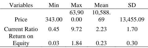
Table 1. Descriptive statistics of variables.
Variables Min Max Mean SD
Price 343.00
63,90 0.00
10,588.
69 13,455.09
Current Ratio 0.45 9.72 2.23 1.70
Return on
Equity 0.03 1.84 0.23 0.30
Table 1 shows the descriptive statistics of the price (P), current ratio (CR) and returns on equity (ROE). The minimum price of LQ45 stock is IDR 343, and the maximum price is IDR 63,900 with the average IDR
www.ijiset.com
4
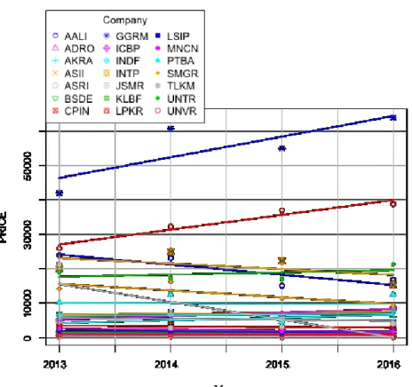
Figure 1. Temporal trend of stock price for each firm (2013-2016)
Some firms have high stock price over 2013 to 2016 and some firms have lower stock price. Every firm seem has linear temporal trend where with some of firms have a positive gradient and the other have negative gradients. The high variability of stock price over firms might and there is no non-linear temporal trend be modeled by means panel data analysis.
There are three candidates model will be evaluates induced: pooled, fixed and random effect model. Two different estimators will be applied, frequentist and Bayesian INLA approaches.
3.3. Data panel modeling
There are three type of panel data model will be constructed: pooled, fixed, and random effects models. We applied frequentist estimator and Bayesian INLA to model panel data included pooled, fixed and random effects models. The results are shown in Table 2.
Table 2. Parameters estimate of panel model by means least square and INLA methods
Parameter
Least square INLA
Pooled Fixed
Effect
Random
Effect Pooled
Fixed Effect
Random Effect
Intercept 10.1315
(0.3552)
8.9548 (0.3090)
10.1315 (0.3491)
8.9467 (0.2931)
log(Current Ratio) -0.1541
(0.1962)
0.0976 (0.1390)
0.0495 (0.1339)
-0.1541 (0.1928)
0.0994 (0.1380)
0.0533 (0.1233)
log(Return on Equity) 0.8210
(0.1875)
0.2060 (0.0885)
0.2434 (0.0883)
0.8210 (0.1843)
0.2034 (0.0879)
0.2402 (0.0811)
Note: (.) its standard error estimate
Table 3. Model comparison by means frequentist approaches
Test Statistics Decision
Pooled vs Fixed
HR0R: Pooled effect model
HR1R: Fixed effect model
F = 55.182,
dfR1R = 20,
dfR2R = 61,
p-value < 2.2e-16
Reject HR0
Fixed vs Random
HR0R: Random effect model
HR1R: Fixed effect model
Chisq = 132.91, df = 2,
p-value < 2.2e-16
Reject HR0
Table 4. Model comparison by means Bayesian approaches
Model DIC MAE RMSE RP
2
MPL
Pooled 264.5446 0.9079 1.1275 0.2231 -132.1164
Fixed 60.3781 0.1710 0.2580 0.9592 -32.08262
Random 57.8861 0.1744 0.2593 0.9319 -32.53193
www.ijiset.com
5
Table 5. Pseudo Bayes Factor
Test PBF Decision
Pooled vs Fixed
MR1R: Pooled effect model
MR2R: Fixed effect model
𝑃𝐵𝐹12= exp�MPL(𝑀1)−MPL(𝑀2)� = 0
MR2R: Fixed effect model
Pooled vs Random
MR1R: Pooled effect model
MR3R: Random effect model
𝑃𝐵𝐹13= exp�MPL(𝑀1)−MPL(𝑀3)� = 0
MR2R: Random
Fixed vs Random
MR2R: Random effect model
MR3R: Fixed effect model
𝑃𝐵𝐹23= exp�MPL(𝑀2)−MPL(𝑀3)� = 1.567
MR2R: Fixed effect model
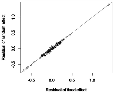
Table 2 shows the parameters estimate of panel model by means least square and INLA methods. The results are almost similar between frequentist and Bayesian methods. Table the model comparison by means frequentist approach. Using Chow test and Hausman test (chi-square), fixed effect model is the best model. Hausman test is strongly support that the fixed effect is better than random
effect. Table 4 and 5 presents the Bayesian model selection criterion. Using Bayesian approach, the fixed and random effect models have similar performance. The DIC,
RP
2
P
, RMSEA, and MAE are not significantly different. PBF also presents the small values < 3 which indicates both of model have similar performance.
Figure 2. Model evaluation of fixed effect
Figure 3. Model evaluation of random effect
Figure 4. Residual of fixed effect vs random effect
www.ijiset.com
6
5. ConclusionThe Hausman may be misleading for some conditions. If the number of time points greater than number of cross-section unit, the Hausman-test tends to wrongly reject the Null-hypothesis of uncorrelated unit effects. Bayesian numerical analysis by means integrated nested Laplace is the one alternative that can be used to model panel data. Bayesian approach provides several criteria for model selection between pooled, fixed and random effect model. Those criteria are deviance information criterion (DIC) and marginal predictive likelihood (MPL) and Bayes Factors (BF). Using Bayesian approach we have similar parameters estimates result with least square approach. However, Bayesian approach found that the fixed effect and random effect models have similar performance in modelling stock price. This result is very different from Hausman statistics which informed that fixed effect model is the best model. However, there is no high different in parameters estimates between fixed and random effect model. Those models concluded that only return on equity has significant effect on the stock price LQ45.
Acknowledgments
This paper is funded by the RFU Unpad contract: 1732 d/UN6.RKT/LT/2018. The authors thank Rector Universitas Padjadjaran and to the anonymous referee whose valuable checking has improved this paper
Reference
[1] R. v. d. Schoot, D. Kaplan, J. Denissen, J. B. Asendorpf, F. J. Neyer and M. A. v. Aken, "A Gentle Introduction to Bayesian Analysis: Applications to Developmental Research," Child Development, vol. 85, no. 3, p. 842–860, 2014.
[2] F. J. Samaniego, A Comparison of the Bayesian and Frequentist Approaches to Estimation, New York: Springer, 2010.
[3] B. H. Baltagi, Econometric Analysis of Panel Data, West Sussex: John Wiley & Sons, 2005.
[4] J. M. Wooldridge, Econometric Analysis of Cross Section and Panel Data, Massachusetts London: The MIT Press, 2001.
[5] W. H. Greene, Econometric Analysis, New Jersey: Prentice Hall, 2006.
[6] U. Morawetz, "Bayesian modelling of panel data with individual effects applied to simulated data," University of Natural Resources and Applied Life Sciences, Vienna, 2006.
[7] K. A. Bollen and J. E. Brand, "A General Panel Model With Random And Fixed Effects: A
Structural Equations Approach," Soc Forces, vol. 89, no. 1, pp. 1-34, 2010.
[8] Hausman, "Specification Tests in Econometrics," Econometrica, vol. 46, no. 6, pp. 1251-1271, 1978. [9] C. Cameron and P. Trivedi, Microeconometrics
Methods and Applications, New York: Cambridge University Press, 2005.
[10] T. S. Clark and D. A. Linzer, "Should I Use Fixed or Random Effects?," Political Science Research and Methods, vol. 3, no. 2, pp. 399-408, 2015.
[11] T. Sheytanova, "The Accuracy of the Hausman Test in Panel Data: a Monte Carlo Study," Orebro University, Sweden, 2004.
[12] G. Koop, D. J. Poirier and J. L. Tobias, Bayesian Econometric Methods, New York: Cambridge Press, 2007.
[13] J. P. LeSage, "Spatial econometric panel data model specification: A Bayesian approach," Spatial Statistics, vol. 19, no. 1, pp. 122-145, 2014.
[14] A. Gelman, J. Hwang and A. Vehtari,
"Understanding predictive information criteria for Bayesian models," Stat Comput, vol. 24, no. 1, p. 997–1016, 2014.
[15] M. Blangiardo and M. Cameletti, Spatial and Spatio-temporal Bayesian Models with R - INLA, Chichester: John Wiley & Sons, 2015.
[16] I. Jaya, H. Folmer, B. N. Ruchjana, F. Kristiani and A. Yudhie, "Modeling of Infectious Diseases: A Core Research Topic for the Next Hundred Years," in Regional Research Frontiers - Vol. 2 Methodological Advances, Regional Systems Modeling and Open Sciences, USA, Springer International Publishing, 2017, pp. 239-254.
[17] I. Jaya, H. Folmer, B. N. Ruchjana, F. Kristiani and Y. Andriyana, "Modeling of Infectious Disease: A Core Research Topic for The Next Hundred Year," in Regional Research Frontiers, US, Springer, 2017, pp. 681-701.
[18] C. Hsiao, K. Lahiri, L.-F. Lee and M. H. Pesaran, Analysis of panels and limited dependent variable models, Cambridge: Cambridge University Press, 2004.
[19] M. Blangiardo and M. Cameletti, Saptial and Spatio-Temporal Bayesian Model with R-INLA, John Wiley: United Kingdom, 2015.
[20] D. J. Spiegelhalter, N. G. Best, B. P. Carlin and A. v. d. Linde, "Bayesian Measures of Model Complexity and Fit," Journal of the Royal Statistical Society. Series B (Statistical Methodology, vol. 6, no. 4, pp. 583-639, 2002. [21] A. E. Gelfand, H.-J. Kim, C. Sirmans and S.