Mean reversion in asset prices and asset allocation in investment management

MEAN REVERSION IN ASSET PRICES

AND ASSET ALLOCATION IN

INVESTMENT MANAGEMENT

Keith Allen Hart

Thesis for the Degree of

Master of Science

Department of Computer and Mathematical Sciences

Faculty of Science

TABLE OF CONTENTS

Abstract iv

Glossary of Terms v

Chapter One : Introduction and Overview 1

1.1 Background 1

1.2 A i m s and Objectives 2

1.3 Outline of the Document. 4

Chapter Two : Survey of the Literature 6

2.1 Introduction and Early Studies 6

2.2 T h e Distribution of Stock Prices 7

2.3 Market Efficiency 9

2.4 M e a n Reversion and the Use of Linear Models 10

2.5 Non-Linear Modelling 13

2.6 Asset Allocation: Theory and Practice 15

2.7 Impact on Investment Strategy 21

Chapter Three : Data Analysis and 23

Autocorrelation: Persistence and Reversion

3.1 Introduction 23

3.2 Sources of Information 23

3.3 Data Analysis 26

3.2.1 Preliminaries 26 3.2.2 Autocorrelation and Persistence 30

3.5 Monthly Results 45

3.6 Validity of the Results: A Sign Test 50

3.7 Conclusion 52

Chapter Four : Mean Reversion Models 53

and the Distribution of Prices

4.1 Introduction 53

4.2 A R D M A and Integrated Linear Models 53

4.3 Model Building - S o m e Empirical Considerations 62

4.4 Model Building 65

4.5 A n Empirical Study In M e a n Reversion 68

4.6 Non-Linear and Other Linear Models 75

4.6.1 Non-Linear Models 75

4.6.2 Outliers 80

4.6.3 Heteroscedasticity 80

4.6.4 A n Actuarial Approach 84

4.6.5 Summary 86

4.7 T h e Distribution of Stock prices 86

4.8 S o m e Results from the Major Asset Classes 90

4.9 Conclusion 96

Appendices 98

Chapter Five : Timing, Theory and Practice 103

5.1 Introduction 103

5.2 Asset Allocation 104

5.3 Data 107

5.4 S o m e Definitions 108

5.5 Industry Background 113

5.6 Portfolio Performance and Ranking's 116

5.7 Attribution Analysis 121

Appendices

₁₃₇

C h a p t e r Six : Conclusions and Future Directions 146

6.1 S u m m a r y of the M a i n Propositions 146

6.2 Impact of the Conclusions 150

6.3 Future Directions 154

Abstract

This thesis examines the predictability of asset prices for an Australian

investor. Evidence supporting the mean reversion alternative to the random walk

hypothesis is presented, with a discussion of potential models, both linear and

non-linear. The normality and homoscedasticity assumptions are investigated and their

use in asset models is validated A study of fund performance is carried out and value

is found to be added by timing asset allocation but not by stock selection, though

there is no correlation between past and present rankings of managers. The difficulty

of proving mean reversion or reversion to trend, other than for large deviations or

extremes, and the actual performance by managers, implies a strategy of allocation at

these extremes. That is, managers should adhere to their policy portfolios and let

markets run short term; making appropriate large strategic moves when markets have

Glossary of Terms

Attribution analysis: The process that attempts to attribute performance to

different components in the overall returns. T h e information is culled from the

respective funds management databases and collected and collated into useable form.

Asset Liability Study: The process by which the assets and liabilities of a

particular fund are examined. Legal liabilities in terms, say, of pension benefits are evaluated against the assets available to pay for those benefits at s o m e time in the future.

Efficient Markets Hypothesis (EMH): A security market in which market

prices fully reflect all k n o w n information is called efficient. T h u s an investor cannot m a k e a gain from a mispriced security.

Financial Reserving: The technical process whereby, usually actuaries, set the

level of reserves needed to meet future claims. These claims, which m a y not have actually arisen yet, are forecast on a statistical basis.

Fundamental Analysis: An analysis of security or asset prices based upon a

detailed study of the asset under question to discern a difference between the value of the asset and its price. This assumes that markets d o not price assets correctly; hence they are 'inefficient'.

Market Timing: The approach by fund managers to attempt to add value to a

portfolio by moving in or out of asset classes, w h e n the relative performance of one class is expected to be better than that of the one m o v e d out of

Mean Reversion: The approach that postulates that security prices will revert

Policy portfolio: This is the benchmark allocation a m o n g asset classes

determined by the manager, representing the managers stance in the market or particular client objectives.

Random Walk: The concept that movement in a variable is unaffected by

previous values of the variable. H e n c e the best forecast of the next value of the variable is the preceding value.

Random Walk Hypothesis: The theory that security prices contain no memory,

in that the best forecast of the next price is the preceding price. It provides the null hypothesis for alternative hypotheses.

Return from market timing: This is the difference between the actual and

benchmark asset allocation for each sector multiplied by the sector benchmark return. This is done each m o n t h and summed.

Return from security selection: This is the difference between the return of the

fund and the sector benchmark return multiplied by the actual asset allocation. This is done each month and s u m m e d .

Security Selection or Selectivity: The approach by fund managers to attempt

to add value to a portfolio by superior selection skills of securities within an asset class.

Sector benchmark return: This is the return of an appropriate index

representing movements in the asset class as a whole. For example, the All Ordinaries accumulation index would represent a suitable benchmark for Australian equities.

Semi-Strong Form Market Efficiency: All publicly available information is in

Strong Form Market Efficiency: All public or private available information is in

the current market price of a security, hence an analysis of such information cannot be used as a basis for earning abnormal returns.

Technical Analysis: An analysis of security or asset prices based upon

historical charts of security prices, hence it is also called 'charting'. Chartists attempt to predict future prices based u p o n particular chart patterns. Essentially future prices are held to be predictable from past history, without any reference to the underlying security.

Variance Ratio Test: The test employed to investigate mean reversion.

Essentially it tests for small autocorrelations at long lags which b e c o m e significant by accumulation. This uses the feature that under the null hypothesis the variance is linear in the lags.

Weak-form Market Efficiency: The information contained in the past sequence

C h a p t e r 1: Introduction and Overview

1.1 Background

In recent years there has been a sharp increase in the study of financial markets. T h e growth in financial services, itself an outpouring both of the growth in computing p o w e r and growth in world trade, and hence integration of international capital

markets, is the fundamental driver of this activity. H e n c e the range of available assets has g r o w n in line with these developments, presenting those w h o m a n a g e these assets with both the opportunities offered by this choice and the problems inherent in dealing with them.

From an historical perspective the major topic of interest has usually been share prices, though it is fair to say that the general public or professional fund managers, have only b e c o m e active in this asset class in m o r e recent times. Physical property and securitised property (via property trusts) are also relatively recent additions. Finally, the whole arena of international investing has opened u p in the last ten years (as indeed is the case with derivative markets). Thus logically investors are n o w presented, not only with the question of which particular security to buy, but which type of security, that is which asset class1 to be in, and when.

Thus we are brought to a consideration of timing. Which asset class should we be in and w h e n ? If security prices are random then prima facie it is futile to attempt to time m o v e m e n t s between asset classes. If however security returns exhibit a long term mean, then there will be periods of time or financial eras w h e n returns are well above long term averages. So, to compensate there will be periods w h e n returns are well below long term averages. If this is so, then prices can be said to be mean reverting. Then it also follows that if an investor is wise enough to be able to anticipate these

1

periods of over or under performance, then that investor will be able to take advantage of this propensity.

The topic of mean reversion or long memory is much debated in the field of econometrics. T h e persistence or otherwise of "shocks" to the economic system are central to debates about the nature of unemployment for example. Is there a 'natural' level of unemployment or does the overall level vary? The same is true for m a n y other economic variables as well as financial asset prices. The answers to these have

profound implications for economic management to say nothing of the particular case of institutional funds management. Thus in some senses part of what w e are

considering is a subset of a m u c h larger topic. W e must be aware of this but cannot take the discussion too far, since it will detract from our central objective.

1.2 Aims and Objectives

In a very real sense investment management is a practical pursuit. Money must be managed. Trustees of superannuation funds, as the law stands, have an obligation to provide an investment strategy. Hence they need a basis upon which to m a k e a policy decision. This is no less true for a small private client than for a manager of the largest funds in the country. W h a t advice can w e therefore offer? W h a t conclusions does the evidence suggest? W h a t do investors actually do and are they successful at it?

We may specify this in more concrete form. Then we will be in a position to outline our 'plan of campaign' to achieve our objectives. T h e final chapter will measure h o w well w e have done.

cost if w e are w r o n g in our assessments. T h e very nature of our pursuit implies that w e must build any case w e m a y present from a range of considerations or w a y s of viewing the topic. B y this w e m e a n that perhaps an activity is feasible, yet if the evidence suggests that no one has actually been able to achieve that activity then logic m a y well indicate that it is simply too hard to do. A good example here would be whether or not professional managers can outperform a given index for an asset class, say the

Australian All Ordinaries Index, for shares. T h e evidence is, and herein w e find no differently, they can't. S o w h y waste time trying? Clearly it is feasible, and hope, no doubt, springs eternal, but cannot the time spent on this be m o r e productively used elsewhere?

This approach is essentially a decision theoretic based one. Conceptually within our decision trees, w e are able to ascribe high probabilities to s o m e routes and low ones to others. W e cannot however give numeric values to these quantities; the

subjective element is there. It would be spurious to attempt too m u c h formality in the conclusions; nevertheless order of magnitude tendencies will indicate directions w e must go.

We do not necessarily aim to develop definitive strategies. They will always be dependent on what objectives are sought by individual investors, what level of risk they are prepared to bear and so on. W h a t w e do wish to do is to bring together more closely theory and practice. If w e cannot prove something then at the very least it needs to be recognized. Action m a y well be taken on the basis of uncertainty, but that is so often the case in the real world where one is dealing with applied economics.

Our strategy within this document must then include quite a wide ranging

1.3 Outline of the D o c u m e n t

Herein w e outline the plan of campaign to achieve our objectives. This will provide 'signposts' on the w a y to provide a clear indication of w h y w e have dealt with topics in the w a y w e have, and w h y s o m e things are in and others are left out. It is to be noted at the outset that m a n y of the individual topics are m o r e than rich enough in terms of research to provide enough for a thesis in themselves. Sometimes therefore w e m a y take an issue a certain distance, hopefully enough for our purposes, but no farther. At those appropriate times, any further research is indicated.

We commence with a review of the literature. This is fairly self-contained, and does serve to put the endeavour into s o m e kind of perspective. T h e following chapter then proceeds with a description of the data, both as to sources and any problems there m a y be. The main body of the w o r k then c o m m e n c e s with, after s o m e introductory analysis, a determination of the autocorrelation structure of the major financial asset class time series. Short run positive autocorrelation and long run m e a n reversion are investigated, along with a discussion of their significance. If m e a n reversion does not exist then attempting to time financial markets is not a worthwhile exercise. W e m a y just as well set our overall parameters and leave the asset allocation largely alone.

The next chapter then starts by considering the use of various classes of linear models as an aid in explaining the underlying generating mechanism. S o m e detailed consideration is given to the nature of the process and a model is developed alongside a simulation study to understand better s o m e of the issues involved in significance testing. W e then look briefly at the class of non-linear models, as well as other

approaches, notably h o w an actuary might deal with the task of determining assets and liabilities as part of the financial reserving 2process. Finally, as part of the task of checking assumptions the relevant financial series are reviewed for changes in m e a n and variance as well as the distribution of asset prices.

2

T h e penultimate chapter moves on to an in-depth study of actual performance.

It is vital to understand what managers can actually do. If they have s h o w n an ability to

time markets then w e need to recognise that, even if theory would suggest it is not

provable statistically. A s such the chapter attempts to review a wide range of

performance statistics from overall predictability of performance, to abilities at the

asset class level and the relationship between aggressiveness of m o v e s and timing

ability. T h e chapter concludes with a look at the asset allocation modelling process, by

pulling together the various strands of the preceding w o r k and seeing which elements

are critical and which are not.

In our conclusion, we hope to bring together all the work in preceding

chapters, so that w e m a y achieve our objective of providing s o m e advice to various

types of investor. It is worthwhile reiterating that w e are, m o r e by the nature of the

uncertainties involved, building a case from a range of evidence rather than providing a

particular clinching piece of evidence. Thus w e m a y hope to add s o m e m o r e to this

C h a p t e r 2: Survey of the Literature

2.1 Introduction and Early Studies

At the outset it is important to note that this survey, whilst attempting to lay out research in chronological order, must of necessity cover contiguous areas of

research. Thus w e m a y follow s o m e of the directions that the research has taken, always keeping in mind the ambit of our thesis. O f course, the researchers have not operated in isolation; fruitful areas have shown flurries of activity, as n e w

methodologies or lines of research have flowered. Certain aspects, as in say price distribution have quietened, while non-linear modeling and m e a n reversion currently s h o w great activity. Nevertheless, spin-offs from one area often can rejuvenate

another. W o r k in this field certainly exhibits those characteristics. Hopefully, w e m a y be able to outline the main thrusts of activity in the field and see the linkages, and also their relation to our study.

The random walk hypothesis and it's corollary the efficient markets hypothesis ( E M H ) , has a long and detailed history. T h e topic goes back to Bachelier (1900), w h o first analysed speculative prices in s o m e detail, proposing the distribution of price changes as independent identically distributed normal variables ( as against a

log-normal distribution, see Alexander (1961). Apart from the Cowles Commission in the United States in the 1930's (reporting in 1939) relatively little w a s done on the topic until after W W I I . O n e of the first to s h o w interest w a s Kendall (1953) w h o considered the autocorrelation structure of various financial time series and concluded they were random walks, with the famous exception of the cotton series where he had used averages, thus bringing forward the brief note from Working (1960), where he demonstrated that first differences of averages in a random chain exhibit significant autocorrelation.

attempt to see, for example, whether various trading rules could be applied to successfully "beat the market". K e y articles were collected by Cootner (1964) and published. F a m a in his review of financial markets, pulled together s o m e of these

concepts, with his definitions of forms of market efficiency (see the glossary for a m o r e detailed exposition), for example, w e a k form efficiency (or can a profit b e m a d e solely based o n the previous price history of a particular security). This is also very closely connected to so called technical analysis in asset prices, where predictions are m a d e based solely on charts, and whether this is a futile activity or not.

We also see a move towards the application of other time series techniques to speculative prices by Granger, applying spectral analysis to stock price time series, for example, Granger and Morgenstern (1963). Granger has written comprehensively o n a wide range of issues connected with speculative prices, over a long period of time. T h e eight references given, are a small portion of his research, logically extending into the recent developments in non-linear modeling and fractional differencing.

2.2 The Distribution of Stock Prices

Research was also directed towards an investigation into the distribution of stock prices with various authors beginning to question the assumption of normality. Alexander carried out investigations into the distribution of prices, at the s a m e time as his study o n the viability of profitable trading rules, suggesting non-normality (he also pointed out the distinction between the use of percentage changes and logs).

Mandelbrot (1963) proposed the class of stable Paretian 1 distributions as a better alternative. F a m a (1963) replied to Mandelbrot's thesis by pointing out, for example, the difficulties posed by a class of distribution with an infinite variance (this is one of Fama's earliest contributions in what has been a lifelong involvement in the area). Since then m a n y other authors, and the list is by no m e a n s complete, have carried out similar studies. Praetz (1972), Blattberg and Gonides(1974), Ali and Giacotto (1982), Officer(1972), H s u , Miller and Wichern (1974), have observed that prices have "fat

1

tails" and are m o r e "peaked" than that predicted by the normal distribution. M o s t recently Sterge (1989) has also found evidence of non-normality in futures prices, where one must be aware of premia or discounts to fair value (that is the 'spot' adjusted for the costs of carry) which will colour the issue. Suggestions for various alternative plausible distributions such as the Student t-distribution or the generalised error distribution, have been put forward by s o m e authors. Praetz suggests the

Student-t, as it converges to the normal, and would thus fit the behaviour of individual stocks which then s u m to a index, the index's behaviour then being approximated by normality.

A comprehensive review of possible distributional forms is found in Ali and Giacotto, along with an analysis of the impact of changing m e a n and variance of share prices on the overall distribution. This links closely to the topics of heteroscedasticity in share prices and changes in the overall level of the mean. Clearly, these changes of location and scale can be the cause of non-normality. Ali and Giacotto's study follows that of Boness, C h e n and Jatusipitak (1974), w h o , in a concluding statement,

commented that "The results of our analyses strongly support the hypothesis that parameters of price change processes vary with capital structure changes" (p. 534). Ali and Giacotto, in their study find no significant evidence of changes of location through time but d o find changes of scale (albeit for individual stocks, but over time periods including months). Perhaps the rationale given by Boness et al explains their findings, as indeed it m a y for the results of non-normality observed by other authors.

2.3 M a r k e t Efficiency

Fama's next most significant contribution w a s the Efficient Markets Hypothesis or E M H ( F a m a (1970)). This w a s proposed in his review of financial markets,

mentioned above, where he attempted to synthesize the k n o w n w o r k on asset markets into one hypothesis.2 These concepts give a framework for analysis of speculative prices, and serve to illustrate the nature of the research. H e n c e the various

autocorrelation studies of short run persistence and long run m e a n reversion can be considered as tests of the w e a k form efficiency of markets. Thus, in an Australian context, Officer (1975)3 reviewed the seasonality and general market efficiency of Australian capital markets. This is a fairly detailed study of various aspects of efficiency, where Officer concluded in favour of seasonality for shares but not for bonds. In a m o r e recent paper Groenewald and K a n g (1993) review the w e a k and semi-strong form efficiency of the Australian share market. Their conclusion is in favour of w e a k form efficiency but undecided on the question of semi-strong form.

An even more comprehensive sequel was published by Fama in 1991. This is a review of w o r k in the broad area of financial economics, as it pertains to speculative prices, bringing together the major results, s o m e of which are directly relevant to this study, m a n y of which are not. It does s h o w both the scope of the field but even m o r e so the enormous growth in interest and research conducted since he first wrote in

1970. It is fair to say that in this later w o r k of F a m a , he is m u c h less sure about the efficiency of markets. H e cites m a n y examples of the predictability of share prices (see for example F a m a and French (1988a)). In his latest commentary, in an applied journal, F a m a (1995) looks at specific practice in stock markets, notably technical and

fundamental analysis. This short paper is aimed at the practitioner, where F a m a finds

2

Weak form efficient means prices cannot be predicted solely on the basis of previous prices.

Semi-strong form means that all publicly available information is in the price and Strong form means that all information both public and private is in the price.

3

too little connection between academic and practitioner. H e clearly feels that m u c h market practice has little merit; stock market analysts need to expose their predictions to the ultimate test of demonstrating a track record. In his studies most fund managers certainly have not demonstrated this ability.

This activity should not be seen in isolation from developments in portfolio theory (Markowitz, Sharpe et al) nor from the seminal w o r k on option theory from Black and Scholes. These issues whilst not core topics for this research per se are nevertheless critical. M o d e r n funds management bases its asset allocation to a large degree on the ideas of portfolio theory, using the mean-variance optimiser to set asset allocation guidelines in the context of a specific asset-liability framework. Clearly m e a n reversion in asset prices and non-normality of the underlying price distribution or any potential heteroscedasticity are likely to have a profound effect u p o n any conclusions. Furthermore, the option pricing models of Black and Scholes (see C o x and Rubenstein (1976) p.205 ) rely o n the E M H , and the i.i.d. normal distribution for the logarithm of asset prices.

2.4 Mean Reversion and the Use of Linear Models

The explosive growth in financial services has been fundamental in driving further research, particularly in the above mentioned areas. The advent of the B o x -Jenkins approach, using the A R T M A class of linear models has encouraged m u c h research into m e a n reversion in general economic issues as well as in the specific area of asset prices.

Granger has picked up this topic where he has recognised the limitations on the standard A R T M A linear model. Hosking (1981) in a paper introduced the idea of fractional differencing (or alternatively fractional integration) where he extended the A R T M A class to fractional models that is, using a differencing parameter which is a fraction, say X • These models exhibit slowly declining, but nevertheless small, levels of autocorrelation which accumulate to a significant size, typical of long m e m o r y

These ideas are outlined in s o m e detail in Granger (1980) and Granger and Joyeux (1980), where the characteristics of such models are determined. T h e use of these models as an alternative or a complement to the use of unit root tests (that is tests where a decision is needed as to whether or not a differencing of one or unity is

statistically sufficient for stationarity, and thus whether or not shocks persist) has been picked up by econometricians, for use in developing their models.

In more recent times work has been conducted into shock persistence in a wide range of macroeconomic aggregates. Cochrane (1988) undertook a study into G N P attempting to determine whether an economy operating at a given level which is below it's potential due to a shock will over-correct to return to it's long-run potential path, hence shock persistence. That is, do these aggregates m e a n revert. Cochrane found little shock persistence in G N P suggesting a random walk for that variable. Other authors have found different results. Mayadunne, Evans and Inder (1995), in a very recent study, looked at a wide range of economic time series to investigate such persistence. Generally speaking their results were inconclusive. W h e n considering the order of integration of the series, they found m a n y with orders of integration above and below one. Put another w a y they found it very hard to decide whether or not shock persistence existed.

Poterba and Summers (1988) addressed this topic using U.S. stock prices and found m e a n reverting behaviour, using the variance ratio test. That is they showed that there is initially positive autocorrelation in stock prices followed by negative

proportion of total stock return variance caused by the predictable component. They find the proportion low, ".. ranges from 7 - 1 7 % for the equal weighted N Y S E index, with generally lower values for the value weighted index" (p. 175).

More recently Chou and Ng (1995), extended the mean reversion approach to an analysis of international stock markets, and in particular the short term and long term correlation structure. O n the presupposition that stock prices have a temporary (mean reverting), as well as permanent (random walk) component, they decomposed international stock price indices for six major markets (U.S., U.K., Japan, France, Germany and Canada). They were concerned as to h o w the correlation structure changed over time; based upon the m e a n reversion hypothesis they concluded that the correlations increased over time. Furthermore, they found by dividing the period up into t w o sub-sample time periods that the correlations had increased. That is, there w a s evidence of convergence in the international series because the correlations had

increased.

w h o similarly developed a joint test statistic). T o not consider joint significance, in their view, would be selective bias or 'data snooping' as they term it. T h e net effect of the joint test statistic would be to significantly widen the confidence interval, thus making significant variance ratios n o longer so. P o o n (1995), also employed the joint significance approach applying it to U K data, finding similar difficulties with the m e a n reversion alternative hypothesis. Thus w e m a y see the continuity and development of research in this field.

This study exemplifies the problems. There are many possible tests that can be used. All that is needed is a sampling distribution, obtained either by analytical means or, m o r e likely, using M o n t e Carlo simulation techniques, then the test statistic can b e calculated and the hypothesis tested. Given the difficulty of finding "patterns" in stock prices as against all the noise going on in the market place it is not surprising the results are often inconclusive. This is the m o r e so w h e n it is considered that authors nearly always use the same data, U.S. stock prices, from the C R S P database. S u m m e r s (1986), gives an excellent discussion on this topic, w h e r e he considers in s o m e depth the nature of the difficulties of the issues under study concluding that "..we must face the fact that most of our tests have relatively little p o w e r against certain types of market inefficiency" (p.598).

2.5 Non-Linear Modelling

Having reviewed the literature on linear models, the next logical step is the relatively n e w field of non-linear models. These models are needed because of the difficulty in finding suitable linear models which are capable of representing the facts. That is w e need models where the observations cannot be expressed as a linear

consider an autoregressive model with suddenly changing parameters. Perhaps it is more realistic to use slowly changing parameters to reflect the slower changes in economic circumstances which are likely to exist in reality. There are of course m a n y other potential candidates (covered in depth by Granger and Terasvita (1993) in their most recent book).

The field of applied time series analysis or econometrics has developed an array of potential models in the A R C H class (Autoregressive Conditional

Heteroscedasticity). T h e A R C H model exhibits a form of serial correlation in its variance, thus instead of the variance being constant, it is a function of previous disturbances, say of the form var(vr) = a + (3s ,_,

2

, where e, = yt - \it , and the conditional distribution of yt is assumed normal with m e a n \xt. Harvey (1990) covers the field of econometric analysis in his recent text with an excellent exposition of these recent developments.

In Abhyankar, Copeland and Wong (1995), we find an attempt to deal with non-linearities in financial time series. Other authors of interest in the field of stock prices include Hiemstra and Jones (1994), Nelson (1991) and Scheinkman and LeBaron (1989).

In the Australian context non-linear modeling is pursued by Kearns and Pagan (1993). Their paper is an in-depth study into the volatility of the Australian All

Ordinaries index over the entire period of its existence, that is, from 1875. This paper is itself a logical sequel to extensive studies carried out by Schwert (1989) on the U S market, though he did not apply non-linear techniques. Schwert restricted himself- if this is the correct word - to a wide ranging consideration of market volatility and its possible causes, though his conclusions do suggest the potential of non-linear models. Kearns and Pagan also recognising the heteroscedasticity of their series apply various models to the series for comparative purposes. G A R C H (generalised A R C H m o d e l s ) and E G A R C H (exponential G A R C H ) are used alongside an iterative two-step

"..there is no evidence that the persistence is due to structural change;" over long periods it has remained remarkably constant" (p. 1993).

Before completing our review of the modeling work available it is worth noting

a practical contribution from Wilkie (1992) in the actuarial field, using a 'cascade' style

model. Wilkie allows for m e a n reversion in his real interest rate model, which then helps drive returns from other asset classes and links together the asset-liability side of the picture. T h e merit of the approach is its internal consistency. It also, reflects the fact that insurance companies must have a basis upon which to plan and create their reserves.

2.6 Asset Allocation: Theory and Practice

With our background in the modelling process, we must now shift our focus to asset allocation, the ultimate objective of this research, where w e review the E M H and look at empirical w o r k on asset allocation and review actual performance.

Fama (1991) in the follow up survey to his initial formulation of the EMH in 1970, mentioned previously, recognises that in m a n y w a y s markets are not efficient. There are plenty of indicators which can lead to gain (back to the early studies!). A s regards long-memory he feels results are inconclusive. H e also makes reference to recent research extending factor models to attempt to take into account economic conditions. This is an extension of the Sharpe-Lintner models, where w e are concerned with links between asset classes, rather than just one asset class, and closely linked to the timing issue.

k n o w n inability of sector managers to outperform their respective benchmarks. T h e use of, so called passive management4 approaches has n o w b e c o m e widespread in the U.S. and this is likely to spread elsewhere where identical results apply. It should be noted that this of itself is not a proof of the E M H (perhaps it has m o r e to say about crowd psychology).

In the academic sphere, apart from the contribution from Fama (1972)

discussing the components of investment performance, later papers from K o n and Jen (1979) and K o n (1983) evaluating the investment skills of mutual fund managers, are worthy of mention. It should be noted though, only in the context of equity funds where timing is to be measured against the benchmark of being either in cash or equities. K o n and Jen used a statistical procedure to deduce beta estimates in the equity portfolio (and thus giving changes in tack in the m a n a g e m e n t of the portfolio). This w a s necessary, for at least t w o reasons. Firstly, at that time funds w e r e not invested in a wide range of asset classes, bonds and equities being the extent of the allocation5. Secondly, they lacked the segmental data to be able to determine which area the performance had c o m e from, so they were forced via a m o d e l process to induce w h e n and to w h a t extent the asset allocation switches had occurred. Using this approach with different beta estimates6 they could then deduce h o w successful the managers were by comparing their beta switches with the market results. They could then evaluate the contributions of timing and selectivity. They found that of 3 7 funds tested, 25 had positive selectivity, 5 of which w e r e significant at the 5 % level. With respect to timing they found only 14 of the 3 7 had positive timing estimates and none were statistically significant at the 5 % level. S o m e detailed theoretical discussions on

4

With passive management managers do not pick securities in an asset class, but merely use an index. Thus they are guaranteed the performance of the index, usually at low cost as well.

5

In modern parlance such funds with assets invested in a wide range of asset classes are called 'balanced funds'. Hence, most superannation funds are balanced funds, thus the manager deals with the asset allocation. Large industrial company or public sector funds may well take the asset allocation task 'in-house', and contract out sector management to individual fund managers.

6

the topic, are put forward in the paper by Admati, Bhattacharya, Pfleiderer and Ross (1986), which widens the issue of h o w to evaluate timing and selectivity issues via different models in the absence of a detailed breakdown of the relevant performance data. In the absence of data which can, in s o m e way, attribute performance to

individual sectors, the only alternative is to develop an underlying model structure and apply it to the data. O f necessity this will lead to statistical problems, at the very least, with the conclusions.

Boudoukh (1995) looked at timing ability by examining a sample of asset

allocation funds (thereby sidestepping the issue of timing versus selectivity). H e w a s interested in assessing the timing ability of the managers by seeing whether or not they correctly predicted actual m o v e s in the market. Interestingly, he finds evidence of market timing ability, but "..the evidence is often consistent with such timing ability, but rarely significant from a statistical viewpoint" (p. 14). A very similar situation to the examination of the random walk hypothesis.

Whilst there have been many papers from academics there is also a very

significant and indeed probably the major contribution, from practitioners, particularly from the field of asset consulting, as well as the funds management business. A wide range of these are available, particularly in the applied or industry journals, such as the

Financial Analysts Journal or Journal of Portfolio Management, m a n y of which are

given in the references. There will be m a n y m o r e not listed, m a n y of which are unpublished other than to clients, for example, of stockbroking firms (like M o r g a n Stanley or Solomon Brothers in the U S or J.B.Were and Ord Minett in Australia).

leads to significant outperformance over a buy-and-hold approach; and that generally only " ..modest amounts of information can bring substantial advantage" (p.36).

Klemkosky and Bharati (1995) also attempt a model using various predictive variables, as an aid to timing. Using their model they claim gains, even w h e n transaction costs are taken into account, thereby supporting active portfolio management.

Many practitioners feel that not only can market timing work in theory but that it actually does in practice. Lee and R a h m a n (1991), examined a sample of mutual fund managers. Using their model of returns to identify timing and selectivity they find that "...there is some evidence of superior forecasting ability on the part of fund managers (p. 82). Vandell and Stevens (1989) conducted an empirical examination of the Wells Fargo timing system. They are a very large fund manager in the U.S., with a particular strength in the field of passive funds management. Thus, and most importantly, they were studying an actual fund operation with working systems based upon extensive experience. They concluded that portfolio performance can be improved by market timing. It is noted that the Wells Fargo approach really times extreme markets, that is, any lost opportunities in good markets were m o r e than compensated for w h e n the dramatic downturns occurred. They comment, " A soundly conceived and disciplined approach to timing can reduce downside risk and improve average performance over a cycle" (p.42).

Other papers reviewed include a series initiated by work from Wagner, Shellans and Paul (1992), a team of industry based practitioners -albeit the asset advice

it is worth mentioning a paper by Beebower and Varikooty (1991), w h o point out h o w difficult it actually is to measure market timing ability. Put in an alternative w a y they essentially try to s h o w h o w long it would take to be able to differentiate statistically between genuine skill and just good fortune. Note that one is often trying to measure perhaps 1 - 2 % superior or excess return, and very substantial though that quantity is, it is hard to measure against a background of often quite high nominal returns and large variability of returns. It can indeed take m a n y years to be able to recognise genuine outperformance.

In the Australian context, there are several papers reprinted in the excellent compendium edited by Ball, B r o w n , Finn and Officer (1989), mentioned previously. A paper by Robson (1986), Chapter 30, examines the performance of unit trusts over the period January 1969 to D e c e m b e r 1978, including balanced funds. H e found that the overall performance w a s below his calculated benchmark and there w a s no consistency in performance. H o w e v e r he did find stability in risk levels and correspondence

between risk and objectives. Bird, Chin and M c C r a e (1982), in the following chapter examined superannuation funds and found applying the Jensen measure of

performance, whereby the portfolio performance is adjusted for the level of risk taken, that managers were unable to outperform a passive indexation strategy.

Perhaps on a less formal level, Samuelson (1989,1990), when surveying the results of m a n y years of investment practice, for example managing endowments over a working lifetime, questions the merits of attempting to time markets. In his view there is a lot to be said for what amounts to developing the appropriate asset mix and largely sticking to it. H e also interestingly enough, makes the c o m m e n t that, "I side with Schiller and Modigliani and a m prepared to doubt macro market efficiency", O n c e again it should be noted that even if this statement is true and that m e a n

A s has been indicated above, to be able to achieve our goal of assessing the value of asset allocation or market timing w e must be able to measure it. T h e

techniques applied are based upon the concepts of attribution analysis outlined in the paper by Brinson, H o o d and B e e b o w e r (1986), and the sequel Brinson, Singer and Beebower (1991). T h e basic idea is to be able to separate out sector from asset class performance by attributing to each particular asset, it's return. This enables us to unbundle, as it were, the returns to see the effect of timing, that is the contribution to the total return obtained from being in the right asset at the right time. H e n c e one must have the programs, and other tools necessary to extract the data from fund

management information systems. This is a substantial task, particularly given the incompatibility of most systems. T h e results of the above t w o papers, using this methodology, indicate that active management cost the average sponsor money. They note that whilst s o m e plans added value, by far the most important issue w a s the overall investment policy, that is, the strategic asset allocation. T h e returns from the policy portfolio dwarfed other components. Adding value from timing even where it w a s achieved is not the key issue. Booth and F a m a (1992) in their paper discussing certain technical aspects of returns also suggest that incremental returns m a y actually be lost by active management.

Ankrim (1992) extends the work of Brinson et al, by pointing out that

managers often, in practice, do not stick to their policy portfolios. H e then suggests a risk adjustment procedure that compensates for the extra risk taken (or lower risk if appropriate) by deviating from the relevant benchmark. In essence he compares the portfolio averages to their benchmarks. Whilst his sample is small it is certainly suggestive of a significant level of deviation.

Hensel, Ezra and Ilkiw (1991) in their paper reviewing the importance of the asset allocation decision, point out that asset allocation policy to be accurately

doubt that being in the correct asset class does deliver outperformance, the next obvious questions are w h y , and can w e take advantage.

The paper by Benari (1990) (who is a practitioner) is very interesting as he suggests there are various eras which are m o r e or less appropriate to different asset classes and these eras persist for a long time (although eventually the system, as it were, corrects itself). So, he outlines three periods 1966-72; 1973-82 and 1983-88. T h e key to these eras are the incidence of price inflation. T h e first period can be characterised as one stable but rising inflation. T h e second as accelerating inflation, and the third as declining inflation. Different types of asset did well under each scenario. H e n c e one needed to be able to, correctly, recognise the changed circumstances and act accordingly.

On a more technical level, the paper by Jorion (1992), considers the mean

variance process by which assets are put together in the most efficient manner possible. H e points out that the process of portfolio optimisation, in practice, involves dealing with measurement error, and this means that the optimal allocation obtained should really consist of a scatter diagram of points rather than one clean line.

2.7 Impact on Investment Strategy

Two papers by Thorley (1995) and Reichenstein and Rich (1994), pull together m a n y of the ideas covered in this review. They are interested in what the results of the studies into stock returns, efficiency and m e a n reversion actually imply for market practice. Thorley points out that the use of mean-variance optimisers needs to be treated with caution. H e posits that time diversification (risk can be diversified through time), is not only widely practised, but should be in principle. Using arguments centred on return probabilities he argues for an increasing allocation to risky assets, w h e n a longer time horizon is available. Reichenstein and Rich, justify such a position, not only based upon studies showing the predictability of stock prices, but also on m e a n

diversification benefits outweigh timing ones. H o w e v e r they g o o n to claim that m e a n reversion implies that the actual shortfall risk (of T-notes beating stocks), is m u c h lower than previously thought. This is a function of the lack of independence of yearly returns; and hence they conclude that investors with long time horizons should take a m u c h higher level of risky assets than previously would have been considered

appropriate.

This survey then sets the context for the overall objective of the thesis. That is, having reviewed the random walk hypothesis, m e a n reversion and the modelling of

C h a p t e r 3: Data Analysis and Autocorrelation: Persistence and

Reversion

3.1 Introduction

This chapter commences the main body of the thesis by outlining the sources of information and h o w they are developed to provide our base series for investigation. After considering s o m e key features of the series w e m o v e on to look at the major issues of autocorrelation. W e are attempting to find out as m u c h as possible about the

structure of our financial series and h o w they relate to one another. W e need to consider the extent of any patterns in the series, in particular if they have any long m e m o r y characteristics. Within this context w e must also provide s o m e estimation of the significance of the results, that is h o w m u c h confidence can w e place on our conclusions.

3.2 Sources of Information

The Australian Stock Exchange (ASX) provides information on the All

Ordinaries Index ( A O I ) as far back as January 1875 on a monthly basis. A t that time the index w a s k n o w n as the Commercial and Industrial Index and it continued until June 1936. F r o m July 1936 until December 1979, the index w a s the Sydney All Ordinaries Index; then w h e n the A S X became fully national, the current A O I w a s created. These earlier indices are thus comparable to the current All Ordinaries Index. Potter Warburg1 provided an A O I series back to 1900, and original data w a s added on to take the series back to 1875. T h e Potter Warburg series being re-based w a s

validated against the Commercial and Industrial Index. A n accumulation index is not available over that time. H o w e v e r , one commencing in October 1960 w a s provided by

1

Potter Warburg. Therefore the task w a s to find an appropriate dividend yield series to fill in the missing portion. It is noted that the accumulation index used w a s with month end prices, rather than the average prices given, for example, in the Stock Exchange

Journal. Whilst w e can be confident about the integrity of the Potter W a r b u r g series

from 1960, further back w e cannot be so certain, particularly with the old Commercial and Industrial Index, where the information is in typed foolscap sheets from a ledger. However, the analysis following in 3.3.2, leads us to conclude that it is very likely so. A month end A O I w a s m a d e available, by courtesy of J.B.Were, for the period of the n e w index, that is D e c e m b e r 1979 up to the current time. Prior periods are m o r e difficult; a weekly series from 1968 to 1979 w a s available. Unfortunately, though it w a s adjusted to be comparable to the monthly series2, the weeks ending do not coincide with the month end. Thus w e have variously 4 and 5 w e e k months, so they are not comparable.

A dividend yield series w a s available from the A S X for the period 31 October 1882 to 30 September 1983 which was, however, an unweighted quarterly series . This series w a s first converted to a monthly basis by taking the quarterly rate on an annualised basis and determining the corresponding monthly rate, that is, raising to the power (1/12). Thus the monthly rates for the months in each quarter are identical. A n accumulation index w a s then formed by applying the dividend yield series to the A O I determined above. Finally the accumulation index is reconciled to the current All Ordinaries Accumulation Index which is based u p o n a weighted dividend yield. W e will denote the All Ordinaries Accumulation Index as A O I A , as distinct from the A O I capital series.

' The steps of reconciliation were as follows. Firstly the ratio of the two series w a s taken for the period of overlap being 31/10/1960 to 30/9/83 . This series shows a decreasing trend, due to the bias in unweighted series. B y applying the unweighted yield to the original A O I A series significant shift is apparent by 1983. T h e reason for this is that s o m e larger companies have low dividend yields (examples would be N e w s

2

Corporation and B H P ) and thus the unweighted yield overstates the true yield across the market.

This trend in the series was thus projected back over the previous years, from 31/10/1960 to 31/10/1882. A n d so the original unweighted yield series w a s adjusted by applying this trend to it. There m a y be s o m e bias in this, because of the increasing importance of generally l o w dividend paying mining stocks in the index from the

mid-1960' s. H o w e v e r most of the variance in the series comes from changes in prices not dividends which were extremely stable throughout the period. In any case, a statistical analysis into both series w a s conducted to see whether any results would be affected by this. T h e evidence suggests there is little difference.

The consumer price index (CPI) was obtained from the Australian Bureau of Statistics ( A B S ) . Annual data w a s available from 1850 to 1993 using a long term linked series generated by the A B S (originally the series w a s called the Retail Price Index and contained only basic items like food, clothing and rent). Quarterly data w a s available from 1948. This w a s converted to monthly data by the same method as w a s used on the dividend yield series.

To obtain excess 3returns it was necessary to find a risk free rate. An obvious choice, widely used in funds management, is the 90-day Treasury note. This series w a s m a d e available by the Reserve B a n k of Australia ( R B A ) . T h e earliest date that this series started w a s N o v e m b e r 1959. O f course, in the early days the note rate w a s virtually constant, remaining in the 3 - 4 % band until April 1965. Whilst the series showed a slowly rising trend during the 1970's, it did not exhibit significant volatility until the 1980's, particularly after the $ A w a s floated (and thus exposing short term rates to market forces).

Data for the Commonwealth Bank Bond Index (CBBI) All Maturities and the M o r g a n Stanley Capital International Index ( M S C I I ) w a s m a d e available via the " S U P E R C M S " database. This is an actuarial style database provided by consulting actuaries from a division of Rainmaker Australia based in Sydney . This database

3

provides a large variety of financial time series of varying periods . H o w e v e r despite

the relative shortness of many of the series (the C B B I starts in December 1976 and the

M S C T I in December 1969) they are nevertheless essential if one is to consider

alternative asset classes. It is also of note that only the last 2 0 years of data, for the

bond market, is relevant due to the controlled nature of the market prior to that period.

It could also be argued that the floating of the A $ meant that prior periods were so

different as to m a k e comparisons very difficult.

3.3 Data Analysis

3.3.1 Preliminaries

A s a preliminary, basic statistics on the nature and distribution of the A O I A

accumulation series w a s determined. It is noted that w e will focus throughout on the

total returns, given by the accumulation index for each asset class, because these are

benchmarks for the asset classes, discussed later. Hence, bond returns given by the

C B B I are inclusive of interest payments. Thus w e will define throughout >

(z —z _) _ 1 "

r. = — — x 1 0 0 % and r=—J\rt is the m e a n return.

*,-i » %

where zt is the accumulation return at time t, corresponding to the capital value

denoted pt with dividends re-invested.

The series were examined for non-normality, heteroscedasticity (note that these

will be dealt with in greater depth in Chapter 4) and the existence of significant

autocorrelations, all of which could cause problems with the assumptions in financial

600 «|

Hstogramof MortNy%ChangeAII Ordinaries Accumiation

lnd«CWB82-Feb-B95

%change Intervalsare2.5%v«de

Figure 3.1 Histogram A O I A monthly : Intervals are 2.5% wide

A s can be seen from the above histogram the distribution of monthly

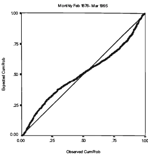
Normal PPRot of MortNy %change All Ords Index

Monthly Feb "B7B- Mar S 9 5

too*

u "8

0.00

too

Figure 3.2 Normal Probability Plot A O I A

T h e cumulative plot shown above gives an alternative w a y of viewing the preceding histogram. There are too m a n y observations centred close to the m e a n and too m a n y extreme values. In part this is likely due to the change in volatility over time. H o w e v e r to assess this, a check on the assumption of constant variance w a s made.

We then need to consider how we are to best measure the variance. A recursive style estimate w a s m a d e , corresponding to an increasing sample size as m o r e data points are added and w e allow time for the series to run-in. T h e estimate is

then:-1 ' _ :

^

=7E(

tVx

«-

)

Given our estimator there will inevitably be time needed for it to settle d o w n as, clearly, data points have a m u c h greater ability to m o v e the series in the earlier period. After s o m e consideration, it w a s felt that the best w a y to capture the longer term movements w a s to determine the 5 year simple moving average of the variance, centred with 3 0 months before and after. T h e estimator4 then becomes:

4

* + 30

I f + JU

60 i= 1-30

There are m a n y other alternative estimators that w e could use, say, a 12-month rolling estimator, or one based u p o n the variance within a calendar year. These shorter term estimates would be very volatile with smoothing required. T h e recursive estimator used does have the virtue of incorporating all the information in the latest estimates. T h e resulting plots are s h o w n in Figures 3.3 and 3.4 below.

Variance: All Ords Accumulation Index Recursive Estimator Monthly 1882-1995

o

e

m

ra

1883 1903 1923 1943 1963 1983

Figure 3.3 Plot of Variance AOIA; Recursive Estimator

70

Variance: All Ords Accumulation Index 60-month Rolling Estimator Monthly 1882-1995

1883 1903

Apart from the period during the 1930's w h e n the volatility5 w a s substantially higher, the variance has fluctuated between 5 % and 1 0 % until the 1960's. Indeed it is noteworthy the w a y it returned to the long term trend after the "shock" of the crash in

1929 died away. It is clear that the volatility had increased significantly during the 1960's (likely related to the increase in the mining component of the A O I ) . T h e period of rapid ascent took place in the late 1960's (Poseidon and the nickel b o o m ) ,

punctuated by the increases d u e to the fallout of 1974 ; the "commodity b o o m " during the late 1970's and m o s t recently the stock market crash of 1987.

It would therefore appear that there has been a permanent increase in volatility in the Australian market. A n d thus w e m a y divide up the history into t w o distinct periods. If w e , s o m e w h a t arbitrarily, take our dividing line as w h e n the variance first exceeded 2 0 % , September 1967, then u p until then the variance w a s 7 . 0 % and since then it has been 3 6 . 6 % , though clearly there is m u c h m o r e variation than this. W e will review this in m o r e detail in 4.5.3, where at a micro level one can discern greater variation. T h e paper by Kearns and Pagan (1993) also covers this topic in considerable depth.

As we shall see later, when considering the variance ratio results, this should not affect the results from 1959 onwards. That is, the period of most interest, the most recent past, has s h o w n a reasonably constant variance, even if at a higher level. Indeed the results are similar for both the m o r e recent period and the whole period.

3.3.2 Autocorrelation and Persistence

T h e next issue to be considered for the series w a s to look for any significant autocorrelations. T h e autocorrelation at lag k is defined b y >

5

Pk =

cov

{var(z,).var(z,_,)}

X

, * = 0,1, , hence p0= l

A correlogram w a s plotted with the following results.

Autocorrelation Function %Change All Ordinaries

AccunmlationlndexOct 1882-Feb 1995

2*

<

0.0"

CorfidenceLirrits

Coefficient 8 9 - 0 1 1 1 2 1 3 1 4 - 6 - B

Lag Nurrber

Figure 3.5 Correlogram A O I A 1882-1995

There are significant autocorrelations at lag 1, with a value of p , = 0.091, and a standard error of 0.027, and again at lags 9 and 14. T h e value of the Box-Ljung statistic for joint significance of the first 12 autocorrelations <2(l2) w a s 29.853, as compared to the critical value of 21.03 for^2o.o5 with 12 degrees of freedom. This further test is a modification of the 'portmanteau' diagnostic test of B o x and Pierce (1970), which tests the joint null hypothesis

#0:Pi =/>2 =•

whereby B o x and Ljung (1978) s h o w that the statistic:

0(K)=n(n

2)±-*

approximately follows the distribution X(K-m)

2

> where m is the number of parameters in the model. In our case m = 0.

However before we attempt to impose some kind of structure on the series we must consider in order

:-1. The partial autocorrelation function (PACF), which measures the correlation between members of a series where dependence on the intermediate terms has been removed. Hence for an A R ( 1 ) all members of the series will be correlated, hence the correlogram will be an exponentially declining series. The P A C F removes that dependence which affects correlations at lag 2, 3,....

2. Is there any difference when we divide up the series into the two periods of differing variances. A s an aside the boundary line was recast back to

30/11/59 to coincide with the period over which the variance ratio tests were conducted.

The partial autocorrelation at lag k is defined

by:-P*

01* = 1 — r ' w n e r e Pk ls t n e (j1 x ^ ) autocorrelation matrix

\pk I

and Pk" is Pk with the last column replaced by (p],p2> Pk)

Filial A utocorrelation Furetion % C h a n g e AII Ordirarie

Accumulation I ndex Oct 1882-Feb S 9 5

Confidence Units

Coefficient

Figure 3.6 Partial Correlogram A O I A 1882-1995

This, in conjunction with the significant autocorrelation at lag 1 in Figure 3.5, suggests that an A R ( 1 ) model m a y b e appropriate, h o w e v e r let us consider item 2 and see if there is any stability in the autocorrelations. O n e w o u l d expect a priori s o m e changes over time.

We have not considered the capital series, the All Ordinaries Index6, over the longer time horizon (see the c o m m e n t s o n this aspect above), h o w e v e r w e should not expect a big difference7, given the stability of the dividend yield series, ranging

between a m i n i m u m of 4 . 4 5 % and a m a x i m u m of 10.29%. Indeed the variance of the dividend yield series w a s a mere 1 . 4 8 % versus a value of 1 2 . 3 7 % for the A O I series, that is the capital component. This difference is even m o r e pronounced for the m o r e recent periods, where, both the volatility o f the capital series has risen and the dividend yield series has, if anything, b e c o m e m o r e stable, due to the tendency for dividend

6

Note that the A S X stated series uses average prices. Based upon the results of Working (1960), where he showed that that the expected first-order serial correlation of first differences between averages of terms in a random chain approximates 0.25 (and using 20 working days per month), we would expect positive autocorrelation. In fact, an analysis gave a value of 0.306 for the period Nov 1959- Feb 1995. W e must therefore use month end data, for any analysis.

7

policy to "smooth" dividends. T o the extent that w e have dividend imputation, and thus an incentive for companies to pay out franked dividends and an increase in smaller investors, this tendency will likely increase. N o t surprisingly, a quick review of the unweighted quarterly dividend yield series, referred to in 3.1, gave a first order autocorrelation of 0.95, a classic A R ( 1 ) representation.

As indicated the series was divided up and the ACF and PACF, for the most recent period w e r e determined with the following

results:-Autocorrelation Function%Change All Ordinaries

Acoxuiation I ndec Nov "B59-Feb ^ 9 5

Confidence Units

Coefficient

<

Fartial A utocorrelation Function % C h a r g e All Ordinarie

Accumiation I ndex N o v 1959-Feb 1995

Confidence Lirrfts

Coefficient

Figure 3.8 Partial Correlogram A O I A 1959-95

T h e A C F in Figure 3.7 exhibits a non-significant level of autocorrelation at lag 1. T h e actual value for the series is px - 0.085 with a standard error of 0.048. T h e m u c h longer series of 1018 observations from Oct 1882 to O c t 1959 gave a value ofp, =0.1028, which is significant at the 5 % level using the standard error calculated of 0.036. This is not greatly different, particularly w h e n one takes account of the October 1987 value, outlined below. Therefore, in this sense it w o u l d appear that the structure and operation of the Australian equity market has not undergone a

significant change. T h e results would suggest positive autocorrelation or persistence, similar to the results of Poterba and S u m m e r s (1988) for the U S market. T h e result is also consistent with the variance ratio results covered in the next section, indicating that perhaps the degree of positive short run autocorrelation is not as strong as that for other smaller markets. This result needs s o m e further qualification, particularly w h e n one considers the results of Groenewald and K a n g (1993). Taking the very m u c h shorter time period of January 1980 (the c o m m e n c e m e n t of the current A O I ) to June

8

1988 they find no significant autocorrelations, or put alternatively the market is weak

form efficient.9

A closer examination of the data reveals some interesting features (these are of course closely related to the heteroscedasticity observed in stock prices that is covered in 4.5.3).

1. There are likely differences in data, so the results herein may well show corresponding differences.

2. As has been shown in the US by Schwert (1989), and in Australia by Kearns and Pagan, large m o v e s in the market tend to be followed by reversals. The series from 1980 to 1988, includes swings of +17.43 to -14.30 to +12.54 separated by a month each time.

3. The period includes the October 1987 large value.

By way of demonstration of the importance of October 1987 in a series of 102 data points, the October value w a s replaced by the m e a n of the t w o either side (as in 4.5.210). T h e value of p , , the first order autocorrelation m o v e d up from 0.038 to 0.111, and p2 went from -0.159 to -0.224 which is significant with a standard error of 0.097. O n e would expect the reversals outlined in item 2 above has a lot to do with the significance of p2. A t the same time the Box-Ljung statistic Q(l2), as defined above, went from 7.736 to 16.132. In effect then w e m a y need to differentiate between

'ordinary' and 'extraordinary' events. Tentatively one might suggest that over the longer period, w h e n individual events are smoothed out or w h e n extraordinary events do not occur, that persistence can be observed. Large reversals or extraordinary events break this pattern to such a degree that they are n o longer statistically observable. Finally, one m a y note the somewhat better results in Groenewald and K a n g of the

9

As outlined in Fama (1970), various forms of efficiency are defined as part of the Efficient Markets Hypothesis (EMH).

10

accumulation series as against the capital ones. This is consistent with "the strong positive autocorrelation observed in the dividend yield series, and should be born in mind w h e n considering the results presented here.

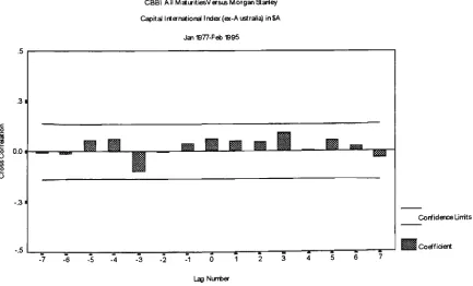
We may summarise these results along with those for the other asset classes, the C B B I and M S C I I , as in the following table. T h e results for the other asset classes are interesting. T h e C B B I exhibits a first-order autocorrelation of 0.116, which is 1.73 times the standard error, not significant, though the Box-Ljung statistic is. T h e M C S T T is far less 'comforting', neither statistic being significant. O f course both series have been subject to considerable change, for the M S C I I devaluations in the 1970's, then the collapse from 1983-85, let alone any reversals. This would merit detailed

Table 3.1 Significance of First - Order Correlation and Joint Significance First 12 Lags for K e y Asset Classes

Series

A O I Accum. Oct 1882- Feb 1995 Ditto - ex Oct 1987

A O I Accum. Oct 1882- Oct 1959 A O I Accum. N o v 1959- Feb 1995

Ditto-ex Oct 1987 C B B I Jan 1977-Feb 1995 M S C I I Jan 1970- Feb 1995 A O I Decl979-Dec 1995

Ditto-ex Oct 1987

A O I Weekly Jan 1968-Dec 1979

P.

* Significant at the 5 % level.

** Significant negative correlation, at the 5 % level, though Q(l2) not so. W e will not address this result herein, but it is certainly interesting .

Given the results in the Table above, one would be inclined to suggest an

AR(1) for the stock series, using the long run series coefficient as parameter; that is a model of the

form:-zt = 0.09lz,_, +s, , st ~N(p,ati 2

) and E(zt)=0 (or else this

is transformed by subtracting z ).

11