Options Pricing and Hedging in a Regime-Switching Volatility Model

(1)

Western University Western University

Scholarship@Western

Electronic Thesis and Dissertation Repository

7-14-2014 12:00 AM

Options Pricing and Hedging in a Regime-Switching Volatility

Model

Melissa A. Mielkie

The University of Western Ontario

Supervisor Dr. Matt Davison

The University of Western Ontario

Graduate Program in Applied Mathematics

A thesis submitted in partial fulfillment of the requirements for the degree in Doctor of Philosophy

Follow this and additional works at: https://ir.lib.uwo.ca/etd

Part of the Finance Commons, Numerical Analysis and Computation Commons, Other Applied Mathematics Commons, and the Partial Differential Equations Commons

Recommended Citation Recommended Citation

Mielkie, Melissa A., "Options Pricing and Hedging in a Regime-Switching Volatility Model" (2014). Electronic Thesis and Dissertation Repository. 2160.

https://ir.lib.uwo.ca/etd/2160

This Dissertation/Thesis is brought to you for free and open access by Scholarship@Western. It has been accepted for inclusion in Electronic Thesis and Dissertation Repository by an authorized administrator of

(2)

VOLATILITY MODEL

(Thesis format: Monograph)

by

Melissa Anne Mielkie

Graduate Program in Applied Mathematics

A thesis submitted in partial fulfillment

of the requirements for the degree of

Doctor of Philosophy

The School of Graduate and Postdoctoral Studies

The University of Western Ontario

London, Ontario, Canada

c

(3)

Abstract

Both deterministic and stochastic volatility models have been used to price and hedge op-tions. Observation of real market data suggests that volatility, while stochastic, is well modelled as alternating between two states. Under this two-state regime-switching framework, we derive coupled pricing partial differential equations (PDEs) with the inclusion of a state-dependent market price of volatility risk (MPVR) term.

Since there is no closed-form solution for this pricing problem, we apply and compare two approaches to solving the coupled PDEs, assuming constant Poisson intensities. First we solve the problem using numerical solution techniques, through the application of the Crank-Nicolson numerical scheme. We also obtain approximate solutions in terms of known Black-Scholes formulae by reformulating our problem and applying the Cauchy-Kowalevski PDE theorem. Both our pricing equations and our approximate solutions give way to the analysis of the impact of our state-dependent MPVR on theoretical option prices. Using financially intuitive constraints on our option prices and Deltas, we prove the necessity of a negative MPVR. An exploration of the regime-switching option prices and their implied volatilities is given, as well as numerical results and intuition supporting our mathematical proofs.

Given our regime-switching framework, there are several different hedging strategies to investigate. We consider using an option to hedge against a potential regime shift. Some practical problems arise with this approach, which lead us to set up portfolios containing a basket of two hedging options. To be more precise, we consider the effects of an option going too far in- and out-of-the-money on our hedging strategy, and introduce limits on the magnitude of such hedging option positions. A complementary approach, where constant volatility is assumed and investor’s risk preferences are taken into account, is also analysed.

Analysis of empirical data supports the hypothesis that volatility levels are affected by up-coming financial events. Finally, we present an extension of our regime-switching framework with deterministic Poisson intensities. In particular, we investigate the impact of time and stock varying Poisson intensities on option prices and their corresponding implied volatilities, using numerical solution techniques. A discussion of some event-driven hedging strategies is given.

Keywords: Analytic Approximation; Coupled Partial Differential Equations; European Option; Hedging; Implied Volatility; Option Pricing; Quantitative Finance; Regime-Switching; Risk Premia

(4)

First and foremost, I would like to thank my supervisor, Dr. Matt Davison, who was instrumen-tal in first sparking my interest in financial mathematics back during my undergraduate thesis. Your constant support and guidance has been invaluable throughout my years as a graduate student. As well, your insight has helped me develop my mathematical and financial intuition, both of which have contributed to my success throughout my education.

I would also like to thank Dr. Adam Metzler and Dr. Mark Reesor, both members of my supervisory committee and of our financial mathematics research group. I have appreciated your insightful feedback of my research over the years.

The financial mathematics Power Hour group was an integral part of why I chose to com-plete my graduate studies in applied mathematics. I would like to thank each and every member of our group. I will always deeply cherish the friendships we have formed and the discussions we have had over the years. I wish you all the best in your future endeavours.

I would like to thank all the students, faculty, and staff from the Department of Applied Mathematics. As a whole, the department has provided a very welcoming and supportive environment which I have greatly appreciated over the years. Whether it be the friendly hellos in the hallway or the fun we have all had at the various social events, I will never forget my time in the department.

My parents, Barbara and Ken, have provided me with their unconditional love and support throughout my education. You have always supported me no matter what path I have chosen and for that I will be forever grateful.

Finally, I would like to thank my fianc´e, Michael, for the love and encouragement you have given me. Without you, I do not think I would have accomplished what I have to date.

(5)

List of Figures

1.1 Historical daily close prices for the S&P/TSX Composite Index. Ticker sym-bol: GSPTSE on the Toronto Stock Exchange. Data obtained from Yahoo Canada Finance [51], covering from April 23, 1984 to March 25, 2014. . . 2 1.2 Distribution of historical daily log returns for close prices of the S&P/TSX

Composite Index. Data obtained from Yahoo Canada Finance [51], covering from April 23, 1984 to March 25, 2014. . . 2 1.3 S&P/TSX Composite Index historical daily log returns. Data obtained from

Yahoo Canada Finance [51], covering from April 23, 1984 to March 25, 2014. . 3

3.1 Comparison of the numerical and true solution for one-dimensional heat equa-tion at timet= 1. All parameters as given in Table 3.1. . . 22 3.2 Comparison of the numerical and true solution for the Black-Scholes PDE at

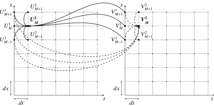
timet= 0. All parameters as given in Table 3.2. . . 24 3.3 Visualization of coupled numerical grids interacting simultaneously to solve

coupled PDEs for a single set of points (U2

M,VM2). . . 25

3.4 Comparison of the numerical and true solution for the coupled one-dimensional heat equation,U(x,t), at timet =1. All parameters as given in Table 3.3. . . 30 3.5 Comparison of the numerical and true solution for the coupled one-dimensional

heat equation,V(x,t), at timet=1. All parameters as given in Table 3.3. . . 31 3.6 Crank-Nicolson numerical solution for the regime-switching coupled pricing

PDEs at timet= 0. All parameters as given in Table 3.4. . . 35

4.1 Comparison of the error estimate for various values ofτ. ε= 0.005, all other parameters as given in Table 4.1. . . 42 4.2 Comparison of the error estimate for various sizes ofε. τ=1, all other

param-eters as given in Table 4.1. . . 43 4.3 Comparison of the numerical and approximate solution of the high state

regime-switching risk-neutral call option att =0. Parameters as given in Table 4.2. . . 57 4.4 Comparison of the numerical and approximate solution of the low state

regime-switching risk-neutral call option att =0. Parameters as given in Table 4.2. . . 58 4.5 Comparison of the backward error associated with solving the state-dependent

Black-Scholes PDEs at t = 0 using the Crank-Nicolson numerical scheme. Parameters as given in Table 4.2. . . 59 4.6 Comparison of the backward error associated with solving the coupled

regime-switching risk-neutral PDEs at t = 0 using the Crank-Nicolson numerical scheme. Parameters as given in Table 4.2. . . 59

(9)

4.7 Comparison of the backward error associated with our approximate regime-switching risk-neutral solution att=0. Parameters as given in Table 4.2. . . 60 4.8 Effect of time on the L2 norm associated with the difference between the

ap-proximate and numerical solutions for the regime-switching risk-neutral cou-pled PDEs. Parameters as given in Table 4.2. . . 60 4.9 Effect of varying the time increments, dt, on theL2 _{norm associated with the}

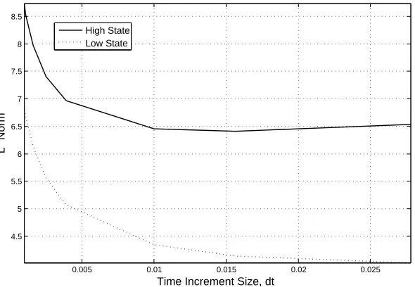
difference between the approximate and numerical solutions at t = 0 for the regime-switching risk-neutral coupled PDEs. Parameters as given in Table 4.2 . 61

5.1 Crank-Nicolson numerical solutions for the coupled pricing PDEs. mHL = −1,mLH =4, all other parameters as given in Table 5.1. . . 72

5.2 Comparison of the numerical and approximate solution of the high state pricing PDE.mHL =mLH = −2, all other parameters as given in Table 5.1. . . 73

5.3 Comparison of the numerical and approximation solution of the low state pric-ing PDE.mHL =mLH =−2, all other parameters as given in Table 5.1. . . 74

5.4 Implied volatility smile corresponding to high and low state risk-neutral regime-switching options prices. mHL = mLH = 0 andS = $100, all other parameters

as given in Table 5.1. . . 75 5.5 State-dependent implied volatility smiles resulting from varying the market

prices of volatility risk. mHL = {0,−1}, mLH = {0,−1}, S = $100, all other

parameters as given in Table 5.1. . . 76

6.1 Example of Portfolio II set-up whenST < K3. . . 93

6.2 Example of Portfolio II set-up whenST > K2. . . 94

6.3 Effect of∆2limit on mean % of trading days with limit breaches. µ = 0%, all

other parameters as given in Table 6.1. . . 111 6.4 Effect of∆3limit on mean % of trading days with limit breaches. µ = 0%, all

other parameters as given in Table 6.1. . . 112 6.5 Effect of ∆2limit on profit/loss of Portfolio II.µ= 0%, all other parameters as

given in Table 6.1. . . 113 6.6 Effect of ∆3limit on profit/loss of Portfolio II.µ= 0%, all other parameters as

given in Table 6.1. . . 114 6.7 Effect of stock price drift, µ, on the mean profit/loss of differing portfolios.

Nlim = 1,T Cstock = 0 bps andT Coption= 0 bps, all other parameters as given in

Table 6.1. . . 115 6.8 Effect of stock price drift, µ, on the mean profit/loss of differing portfolios.

Nlim = 1, T Cstock = 0 bps andT Coption = 10 bps, all other parameters as given

in Table 6.1. . . 116 6.9 Effect of stock price drift, µ, on the mean profit/loss of differing portfolios.

Nlim = 1,T Cstock = 1 bps andT Coption =100 bps, all other parameters as given

in Table 6.1. . . 117

7.1 Two types of event studies: discontinuous stock price movement and volatility regime change. . . 120

(10)

tained from Yahoo Canada Finance [52]. . . 123 7.3 5-day moving average volatility for Apple for fiscal year 2013. Data obtained

from Yahoo Canada Finance [50]. . . 123 7.4 5-day moving average of daily trading volume for TD Bank for fiscal year

2013. Data obtained from Yahoo Canada Finance [52]. . . 124 7.5 5-day moving average of daily trading volume for Apple for fiscal year 2013.

Data obtained from Yahoo Canada Finance [50]. . . 125 7.6 Time varying Poisson intensity assuming the financial event occurs at maturity.

κ=1,λ?= 10% (daily), andT =1 year. . . 128 7.7 Time varying Poisson intensity assuming the financial event occurs before

ma-turity.κ= 1,λ? =10% (daily),τ? =9 months, andT =1 year. . . 129 7.8 Time and stock varying Poisson intensity assuming the financial event occurs

at maturity. Parameters as given in Table 7.3. . . 131 7.9 Time and stock varying Poisson intensity assuming the financial event occurs

before maturity. Parameters as given in Table 7.3. . . 132 7.10 Impact ofκon the time-dependent Poisson intensity assuming the event occurs

at option maturity.λ?= 10% (daily) andT =1 year. . . 133 7.11 Impact ofκon the time-dependent Poisson intensity assuming the event occurs

before option maturity.λ? = 10% (daily),τ? =9 months, andT =1 year. . . . 134 7.12 Comparison of numerical regime-switching option prices between the

bench-mark case and Case 1 att= 0. Parameters as given in Table 7.4. . . 136 7.13 Difference between the benchmark case and Case 1 numerical option prices at

t=0. Parameters as given in Table 7.4. . . 137 7.14 Implied volatility smiles corresponding to option prices for the benchmark case

and Case 1.S = $100, all other parameters as given in Table 7.4. . . 137 7.15 Comparison of regime-switching option prices between the benchmark case

and Case 2 att =0. Parameters as given in Table 7.4. . . 138 7.16 Difference between the benchmark case and Case 2 numerical option prices at

and Case 4.S = $100, all other parameters as given in Table 7.4. . . 145

(11)

A.1 Comparison of benchmark case and Case 1 numerical regime-switching option prices, zoomed about the strike K = $100. Parameters as given in Table 7.4. Original plot depicted in Figure 7.12. . . 155 A.2 Comparison of benchmark case and Case 2 numerical regime-switching option

prices, zoomed about the strike K = $100. Parameters as given in Table 7.4. Figure 7.15 depicts original, non-zoomed plot. . . 156 A.3 Comparison of benchmark case and Case 3 numerical regime-switching option

prices, zoomed about the strike K = $100. Parameters as given in Table 7.4. Figure 7.18 depicts original, non-zoomed plot. . . 156 A.4 Comparison of benchmark case and Case 4 numerical regime-switching option

prices, zoomed about the strike K = $100. Parameters as given in Table 7.4. Figure 7.21 depicts original, non-zoomed plot. . . 157

(12)

List of Tables

3.1 Parameters used in the implementation of the Crank-Nicolson numerical scheme for the one-dimensional heat equation. . . 21 3.2 Parameters used in the implementation of the Crank-Nicolson numerical scheme

for the Black-Scholes PDE. . . 24 3.3 Parameters used in the implementation of the Crank-Nicolson numerical scheme

for the coupled one-dimensional heat equations. . . 29 3.4 Parameters used in the implementation of the Crank-Nicolson numerical scheme

for the regime-switching coupled PDEs. . . 34

4.1 Parameters used in investigation of error estimate. . . 41 4.2 Parameters used in the implementation of the Crank-Nicolson numerical scheme. 56

5.1 Parameters used in the implementation of the Crank-Nicolson numerical scheme. 72

6.1 Parameters used in the analysis of hedging strategies for varying stock price path drifts. . . 106 6.2 Summary of total state occupations and total state transitions for price paths

used in hedging analysis. . . 107 6.3 Hedging analysis for varying stock price path drifts using numerical option

prices. Parameters as given in Table 6.1. . . 108 6.4 Hedging analysis for varying stock price path drifts using approximate option

prices. Parameters as given in Table 6.1. . . 110

7.1 Quarter end and earnings release dates for Toronto Dominion bank for fiscal year 2013. Ticker symbol TD.TO on TSX. Data obtained from [42], [43], [44], and [45]. . . 121 7.2 Quarter end and earnings release dates for Apple for fiscal year 2013. Ticker

symbol APPL on Nasdaq. Data obtained from [1], [2], [3], and [4]. . . 122 7.3 Parameters used in the analysis of time and stock varying Poisson intensities. . 131 7.4 Parameters used in the analysis of option pricing for deterministic Poisson

in-tensities. Note:†_{This event date is only used for Case 2 and Case 4 where it is} assumed that the event occurs before the maturity date of our regime-switching call option. . . 135 7.5 Summary of results for the time varying and time and stock varying Poisson

intensity cases. . . 147

(13)

List of Appendices

Appendix A Additional Deterministic Intensity Analysis . . . 155

(14)

List of Abbreviations and Symbols

List of Abbreviations

• CDF – cumulative distribution function

• GBM – geometric Brownian motion

• MPVR – market price of volatility risk

• PDE – partial differential equation

• SDE – stochastic differential equation

• TC – transaction cost

(15)

List of Symbols

• i, j– volatility states

• t– time

• Ci(S,t) – state-dependent regime-switching call option value, conditional on volatility statei

• Ci

BS(S,t) – Black-Scholes call option value, conditional on volatility statei • S(t) – price underlying asset at timet

• r– risk-free rate of interest

• µ– drift of underlying asset

• σi – state-dependent volatility of underlying asset

• K – strike price of an option

• T – maturity date of an option

• W(t) – Brownian motion

• λi j(S,t) – state-dependent Poisson intensity, driving the switch from volatility state ito

volatility state j

• dqi j(t) – independent Poisson process with probabilityλi j(S,t)dt

• fi j(S,t) – PDE source term coefficient

• mi j(S,t) – state-dependent market price of volatility risk

• X(S,t) – difference between low volatility state Black-Scholes and regime-switching call option values

• Y(S,t) – difference between high volatility state Black-Scholes and regime-switching call option values

• Πi(S,t) – state-dependent hedge portfolio, conditional on volatility statei

• ∆i _{– hedge ratio of a hedging instrument, conditional on volatility state}_i

• Nlim – limit on hedge ratio for hedging option

• T Cstock– transaction cost for underlying asset

• T Coption– transaction cost for hedging options

• σi,imp– state-dependent implied volatility

• Pi,unconditional– unconditional probability of occupying statei

(16)

• κ– time intensity parameter

• τ? – time of financial event

• λ?_{i j} – maximum state-dependent constant Poisson intensity

• N – number of volatility regimes; number of hedging options

• dx,dS,dt – space, stock price and time increment, respectively

• m,l– space/stock and time index, respectively

• M,L˜ – number space/stock price and time increments, respectively

• n,n? – hedging option and additional hedging option index, respectively

(17)

Chapter 1 Introduction

Both practitioners and academics have focused for decades on characterizing the randomness of stock prices and on the underlying market conditions which affect their evolution. One of the factors affecting stock price evolution is volatility: the degree to which prices fluctuate. Volatility has long been known to vary over time in an essentially unpredictable way. Study-ing empirical equity data can provide a way to formulate reasonable and tractable volatility models. This thesis is based on the assumption that volatility is stochastic in a very particular way; it fluctuates between a finite number of regimes. Our focus is on formulating financially appropriate mathematical models to describe the evolution of volatility over time. This thesis does not consider the important and interesting problem of volatility prediction. We will first motivate the existence of stochastic volatility by studying empirical equity data.

Consider a price path such as that for the S&P/TSX Composite Index which is currently composed of 244 of the largest public companies, by market capitalization, trading on the Toronto Stock Exchange (TSX). One can observe an overall trend in the price path which covers from 1984 to 2014, as illustrated in Figure 1.1 for the S&P/TSX Composite Index. It is also immediately evident that daily prices move randomly and it is easy to see how they could be hard to predict.

A common mathematical finance technique for studying stock price paths is to consider the log returns of the asset prices. This allows for us to study the distribution of the returns and to analyse their magnitude. Higher magnitude stock returns are associated with higher volatility in the underlying stock price path. It is commonly thought that stock returns follow, at least approximately, a lognormal distribution and as such this distribution is used as a benchmark model in finance. In general, stock price returns are computed as follows:

u(t+1)=ln S(t+1)

S(t)

!

, (1.1)

whereS(t) is the price of the underlying asset at timet.

First, we plot a histogram containing the stock returns associated with the daily close prices, which are illustrated in Figure 1.2.

(18)

Jan−85 Jan−90 Jan−95 Jan−00 Jan−05 Jan−10 4000

6000 8000 10000 12000 14000

Days

Daily Close Prices

Student Version of MATLAB

Figure 1.1: Historical daily close prices for the S&P/TSX Composite Index. Ticker symbol: GSPTSE on the Toronto Stock Exchange. Data obtained from Yahoo Canada Finance [51], covering from April 23, 1984 to March 25, 2014.

−0.150 −0.1 −0.05 0 0.05 0.1

1 2 3 4 5 6 7 8

Daily Log Returns

Log(Number of Observations)

(19)

3

The histogram shown in Figure 1.2 seems to indicates two magnitudes of stock returns, visible in the separation in the data. It can also be observed that the data do not appear to follow a lognormal distribution. Instead the data appears fat-tailed with outliers on either side of the main data peak. Another way to analyze the data, in order to determine if there are changes in the volatility, is to consider the log returns plotted against time.

Jan−85 Jan−90 Jan−95 Jan−00 Jan−05 Jan−10

−0.12 −0.1 −0.08 −0.06 −0.04 −0.02 0 0.02 0.04 0.06 0.08

Days

Daily Log Returns

Figure 1.3: S&P/TSX Composite Index historical daily log returns. Data obtained from Yahoo Canada Finance [51], covering from April 23, 1984 to March 25, 2014.

Looking at Figure 1.3, which depicts a time series of the daily log returns for the S&P/TSX Composite index from 1984 to 2014 allows us to easily identify periods of abnormal volatility levels. There are several “bursts” observed in the daily log returns. These bursts, which refer to the observable increases in the magnitude of the daily log returns, are associated with increased volatility. After these bursts are observed in the market, they can sometimes be associated with known economic and financial events in history. High magnitude returns in 1987 can be at-tributed to the stock market crash, known as Black Monday, on October 19, 1987. Around the year 2001, increases in volatility levels can be explained by the Dot-Com Bubble and more recently in the years 2007-2008, increases in volatility can be associated with the Subprime Mortgage Crisis. This empirical data indicates that volatility is in fact stochastic and is influ-enced by economic events. Interestingly enough, different economic and financial events could also in return be a trigger for shifts in volatility levels. One part of this thesis involves explor-ing the relationship between increases in volatility levels and the arrival of upcomexplor-ing financial events.

(20)

on an underlying asset following geometric Brownian motion (GBM) with constant drift and constant volatility. Although the constant volatility assumption has now been disproven, their closed-form solution for European options and associated hedging arguments provide for a nice benchmark model for comparison with subsequent options pricing frameworks.

There has been much recent interest on pricing and hedging options written on stocks fol-lowing diffusion processes with random volatility coefficients. Heston [27] was a pioneer in modelling volatility uncertainty, pricing a European option written on an underlying asset, the price of which followed geometric Brownian motion (GBM) with stochastic volatility. He chose his volatility process to incorporate mean reversion which allowed for the process to revert to a long run average volatility level over time at a specified speed. Another popu-lar stochastic volatility model is the Generalized Autoregressive Conditional Heteroskedas-ticity (GARCH) model. Hansen and Lunde [24] compared 330 volatility models, including variations of GARCH and ARCH (Autoregressive Conditional Heteroskedasticity) to forecast out-of-sample intraday volatility for US equity data. Using a variety of statistical tests, they showed that for small time intervals, a Markov regime-switching GARCH with two states out-performed GARCH in forecasting volatility. Although this thesis does not consider parameter estimation for Markov models, much progress has been made in this area, including work by Xi and Mamon [53], [55], and Xi, Rodrigo, and Mamon [54].

Economists have long considered that the business cycle fluctuates between different stages, such as expansion and contraction. Hamilton [22], [23] studied US post-war gross national product (GNP) data and found that growth rates for specific regimes of a Markov process were associated with different business cycles. More recently financial literature has proposed that volatility can be well modelled by shifts between a finite number of regimes. The consideration of the business cycle, as well as observation of market data, suggests that volatility is well modelled by random moves between low and high regimes. Hardy [25] showed that a two-regime lognormal model was sufficient to model equity data, in particular the Canadian Toronto Stock Exchange (TSX), and was preferable over other statistical approaches used in volatility modelling. Furthermore, Filardo [19] used a Markov model with time-varying transitional probabilities to model business cycles, in particular two phases: expansion and contraction.

For simplicity and tractability, as well as for realism, we will consider a two-regime model in which the volatility can switch between high and low regimes. Similarly to Merton’s [32] model, which included Poisson jumps in the stock price dynamics, we model the shifts between regimes by Poisson processes with deterministic intensities. We begin our study of this model with constant Poisson intensities driving the switches between regimes. Later on, the intensities are allowed to vary with time and stock price levels. We set up a hedge portfolio where we take simultaneous positions in an asset and in an option, as suggested by Naik [35], to hedge against our risk exposure. Using Black and Scholes type hedging and standard arbitrage arguments, we derive a system of coupled partial differential equations (PDEs) representing state-dependent option prices in a regime-switching market. Our generalized N-state pricing PDEs have a similar form to those previously derived by Boyle and Draviam [9], Buffington and Elliott [11], Di Masi et al. [15], and Naik [35], with the additional inclusion of a market price of volatility risk term.

(21)

5

and Elliott derived their regime-switching PDE using standard stochastic calculus techniques involving expectations and martingales. On the other hand, Di Masi et al. derived their PDEs using a hedging approach where they assumed that volatility could not be perfectly hedged and thus they hedge by locally minimizing the associated risk. Under the risk-neutral measure, Ma-mon and Rodrigo [31] derived an integral-type solution in terms of the Black-Scholes option prices. Furthermore, Naik reduced the solution for a European call option on a regime switch-ing asset, assumswitch-ing zero market price of volatility risk, to a quadrature. Bollen [7] priced both European and American options, written on underlying assets with regime-switching returns, using a pentanomial lattice.

As a benchmark for our volatility framework and pricing problem, we will consistently consider pricing and hedging a European call option throughout this thesis. We will solve our regime-switching pricing problem both numerically and by using approximation solution techniques. Both methods lead to further analysis of parameters such as the volatility risk premium. It also allows for us to directly compare our model to the constant volatility Black-Scholes model which allows for useful financial intuition of our switching framework.

Several key words arise frequently throughout our investigation of this framework. They are defined below for ease of reading.

• Financial option: Contract which gives its owner the right but not the obligation to buy or sell the underlying asset at a predetermined price (strike price) on or before a prede-termined date (maturity date).

• European call option: Contract which gives its owner the right but not the obligation to buy the underlying asset at the strike price on the maturity date.

• Option premium: Price charged for the option at contract initiation (timet= 0).

• Moneyness: Relationship between the underlying asset’s price and the strike price. It describes the option’s intrinsic value (i.e. the value if the option were to expire today). Options can be in-the-money, at-the-money, or out-of-the-money.

• Hedging: Trading strategy that aims to reduce or eliminate the risk associated with fi-nancial instruments in our portfolio.

• Short position: Position in which an investor has sold a financial instrument to a coun-terparty.

It should be noted that on actual options exchanges such as the Chicago Board Options Exchange, options are usually exchanged for 100 units of the underlying asset [46]. For sim-plicity, we will just assume our option is exercised for one unit of the stock.

(22)

(23)

Chapter 2 Regime-Switching Framework

We start with an introduction to regime-switching models in which the notation used in the subsequent chapters will be introduced. We will consistently consider throughout a European call option with payoff(S(T)−K)+[28], in which we assume the investor takes a short position. An overview of the market in which we are hedging and pricing is given as well as a description of geometric Brownian motion. A detailed discussion of the regime-switching framework follows, first for the generalized N-state, and then for the economically reasonable two-state case.

2.1 Market Assumptions

In order to derive the option pricing and hedge ratio relations in the subsequent sections, certain assumptions about the general market in which we are hedging and pricing options must hold. Many of these assumptions are the same as under the Black-Scholes constant volatility option pricing model [6].

First, we assume our financial market is such that the volatility can switch between a finite number of volatility regimes. The stock price follows geometric Brownian motion while inde-pendent Poisson processes are used to model the jumps between regimes. The expected return will be independent of state and it is assumed that the state-dependent volatilities have constant fixed values. The risk-free rate of interest is also assumed to be constant. Furthermore, it is assumed that we can hedge continuously and buy any quantity of the hedging instruments in our portfolio. This includes both the underlying asset and any hedging options. Finally, in the absence of transaction costs, there exists no arbitrage opportunities. In other words, there is no way for an investor to earn a riskless profit.

2.2 Geometric Brownian Motion

We assume the dynamics of our stock price (i.e. underlying asset) follow a widely used and well known stochastic differential equation (SDE) in mathematical finance, otherwise known as geometric Brownian motion (GBM). The stock price dynamics are as follows under the real world measureP:

(24)

dS(t)=µS(t)+σ(t)S(t)dW(t), (2.1) where dW(t) is an increment of a Wiener process (i.e. W(t) is Brownian motion). The four properties of a Wiener process are as follows:

• W(0)=0,

• W(t+dt)−W(t)∼ N(0,dt) for allt>0 anddt >0,

• all increments are independent,

• W(t) is continuous everywhere but differentiable nowhere.

Recall that in our model the expected return (i.e. drift) of the stock price,µ, is constant and independent of state, while the volatility,σ(t), can switch between a finite number of regimes. The first term in the SDE represents the deterministic growth of the stock price where the drift dictates the overall direction in which the stock price evolves. The second term incorpo-rates randomness into the model, allowing fluctuations in the stock price to vary with the level of risk (i.e. volatility).

2.3 N

-State Case

2.3.1 Regime-Switching Volatility

Given a finite number of volatility regimes,N, assuming volatility occupies volatility state iat time t, there are N −1 possible regimes to which the market can transition to at timet +dt. Therefore at every time point we are exposed to the risk ofN−1 volatility jumps of differing magnitude and direction. It is possible to remain in the currently occupied regime, however there is no inherent risk associated with constant volatility, so no hedging option would be needed in our portfolio if we knew volatility was constant.

Under the real world measure P, the volatility’s stochastic differential equation (SDE) is

governed by:

dσ(t)= σ(t)

N X

j=1

j_,i

Ji j−1

dqi j(t), (2.2)

where

Ji j =

σj−σ(t)

σ(t) +1, (2.3)

andσ(t)=σifori= 1, . . . ,N. Ji j represents the relative magnitude of the volatility jump from

regimeito regime jsuch thati_, jwhereσiis the fixed volatility value for regimei.

dqi j(t)=       

1 with probabilityλi j(S,t)dt

0 with probability 1−λi j(S,t)dt

(25)

2.3. N-StateCase 9

where 0≤ λi jdt ≤1 must old. The independent Poisson processes,qi j(t), are also independent

of the Brownian motion W(t) embedded in the stock price dynamics. The Poisson intensity,

λi j(S,t) controls the likelihood of the jump from volatility stateiat timetto volatility state jat

timet+dt.

2.3.2 Regime-Switching Option Dynamics

We want to consider the dynamics of an option,C(S, σi,t), written on an underlying asset,S(t)

with regime-switching volatility,σ(t). There areN−1 possible regime shifts from each regime

i. This does not include the possibility of remaining in the presently occupied regime.

Using the Itˆo-Doeblin formula for jump processes [39], we derive an expression for the dynamics of our regime-switching option. For simplicity of notation,Ci₍_S,_t₎_≡_C₍_S, σ

i,t) and S ≡S(t).

Under the assumption that the time incrementdtis very small:

dW(t)≈ √

dt ⇒ dW(t)2 _≈ dt,

(2.5)

dW(t)dt ≈0, (2.6)

dt2 _≈

0. (2.7)

We utilize the above results to obtain:

dS2 =µ2_S2 _dt2+

2µσiS2dtdW(t)+σ2iS

2 _dW₍_t₎2 = σ2

iS

2_dt, _(2.8)

and as a result:

dCi(S,t)= ∂C

i

∂S (S,t)dS +

∂Ci

∂t (S,t)dt+

1 2

∂2_Ci

∂S2(S,t) dS

2

+

N X

j=1

j_,i h

Cj(S,t)−Ci(S,t)idqi j(t), (2.9)

⇒ dCi(S,t)= ∂C

i

∂t (S,t)+

1 2σ

2

iS

2∂2C

i

∂S2(S,t)

!

dt+ ∂C

i

∂S (S,t)dS

+

N X

j=1

j,i h

Cj(S,t)−Ci(S,t)idqi j(t). (2.10)

In the generalized N-state case, the regime-switching option is exposed to the risk of the movements in the underlying asset, denoted by the term withdS. This option is also exposed to all possible N − 1 jumps between volatility regimes, since the dynamics depend on terms containingdqi j(t).

(26)

2.3.3 Pricing Equation Derivation

Here we present a detailed derivation of the equations for the value of an option contract written on an asset with regime-switching volatility. The contract price depends, as usual, on the stock price and time, but also on what state the volatility occupies. The result is a system of coupled pricing equations, one for each volatility state. These equations may be developed using standing hedging arguments dating back to Black and Scholes [6], as summarized in Wilmott [49]. These arguments are shown in detail in the succeeding sections for completeness. For simplicity, suppose we are hedging against a position in a plain vanilla option. In particular, we consider an investor who takes a short position in a European call option. We can hedge against the stock price movements by taking a position in the underlying asset. Since the call option with priceCi(S,t) is written on an underlying asset with regime-switching volatility, we need N−1 hedging options to hedge against allN−1 possible volatility switches. This is under the assumption that there are no available instruments that directly hedge volatility risk.

Our portfolio,Πi₍_S,_t_{), consists of a short position in a European call option}_Ci

1(S,t) struck

atK1with maturity dateT1. We can minimize and in some cases offset such risk by dynamically

hedging, where we readjust our hedge position in a portfolio as desired. As a result a position is taken in the underlying assetS andN−1 hedge positions in other call optionsCi

n(S,t) where

n = 2, . . . ,N, written on the same underlying asset but with different contract specifications.

In particular, we require thatTn > T1 for all n = 2, . . . ,N.s In order for the hedging strategy

to be non-redundant, we require that at least one of the strike price or the maturity date of our hedging options differs from the initial shorted call option.

Basic hedging and arbitrage arguments are utilized under our framework to derive the cou-pled pricing equations. This derivation is shown in complete detail below.

Our portfolio can be represented mathematically as:

Πi

(S,t)=−Ci₁(S,t)+ ∆i₁S + N X

n=2

∆i nC

i

n(S,t). (2.11)

We are interested in how the randomness inherent in our portfolio affects the actual change in the value of the hedge portfolio.

dΠi(S,t)=−dCi₁(S,t)+ ∆i₁dS + N X

n=2

∆i ndC

i

n(S,t). (2.12)

The dynamics of all options are the same since they are all written on the same underlying asset with volatility following a regime-switching process. Thus we can apply our result given by equation (2.10) fordCi

n(S,t) for alln=1, . . . ,N. The change in the portfolio value is now:

dΠi(S,t)=− ( ∂Ci

1

∂t (S,t)+

1 2σ

2

iS

2∂ 2_Ci

1

∂S2 (S,t)

!

dt+ ∂C

i

1

∂S (S,t)+

N X

j=1

j_,i h

C₁j(S,t)−C₁i(S,t)i

)

+ ∆i

1dS +

N X

n=2

∆i n

( ∂Ci n

∂t (S,t)+

1 2σ

i S2∂

2_Ci n

∂S2 (S,t)

!

dt+ ∂C

i n

(27)

2.3. N-StateCase 11

+

N X

j=1

j,i h

Cnj(S,t)−C i n(S,t)

i

dqi j(t) )

, (2.13)

⇒dΠi(S,t)=

( − ∂C

i

1

∂t (S,t)+

1 2σ

2

iS

2∂ 2_Ci

1

∂S2 (S,t)

!

+

N X

n=2

∆i n

∂Ci

n

∂t (S,t)+

1 2σ

2

iS

2∂2C

i n

∂S2 (S,t)

!) dt + ( ∆i 1− ∂Ci n

∂S (S,t)+

N X

n=2

∆i n

∂Ci

n

∂S (S,t)

)

dS

+

N X

j=1

j_,i ( N

X

n=2

∆i n

h

i

−hC₁j(S,t)−C₁i(S,t)i

)

dqi j(t). (2.14)

We want to choose our hedge ratios,∆i

n, in such a way that the randomness associated with

the stock price movements and the volatility switching is eliminated. This is done by setting the hedge ratios so that the groups of terms associated withdS and with alldqi j(t) vanish.

Thus, to hedge against movements in the underlying asset, choose:

∆i

1 =

∂Ci

1

∂S (S,t)−

N X

n=2

∆i n

∂Ci

n

∂S (S,t). (2.15)

To hedge against all possibleN−1 volatility jumps at timet,

N X

n=2

∆i n

h

i

−hC₁j(S,t)−Ci₁(S,t)i= 0, (2.16)

for all j= 1, . . . ,N, j,i. (N−1 equations)

Since we hedged out all the risk associated with movements in the underlying asset and with jumps in volatility, the value of our portfolio only depends on the deterministic change in time. Therefore we can set the change in portfolio value equal to the risk-free return on the portfolio.

dΠi(S,t)=rΠi(S,t)dt, (2.17)

( − ∂C

i

1

∂t (S,t)+

1 2σ

2

iS2

∂2_Ci

1

∂S2(S,t)

!

+

N X

n=2

∆i n

∂Ci

n

∂t (S,t)+

1 2σ

2

iS2

∂Ci

n

∂S2(S,t)

!)

dt

=r

(

−Ci₁(S,t)+ ∆i₁S + N X

n=2

∆i nC

i n(S,t)

)

dt, (2.18)

− ∂C i

1

∂t (S,t)+

1 2σ

2

iS

2∂ 2_Ci

1

∂S2 (S,t)

!

+

N X

n=2

∆i n

∂Ci

n

∂t (S,t)+

1 2σ 2 iS 2∂C i n

∂S2(S,t)

!

=−rCi₁(S,t)+rS ∂C i

1

∂S dS −

N X

n=2

∆i n

∂Ci

n

∂S (S,t)

!

+

N X

n=2

∆i nrC

i

n(S,t), (2.19)

⇒ − ∂C i

1

∂t (S,t)+

1 2σ

2

iS

2∂ 2_Ci

1

∂S2 (S,t)+rS

∂Ci

1

∂S (S,t)−rC

i

1(S,t)

(28)

+

N X

n=2

∆i n

∂Ci

n

∂t (S,t)+

1 2σ

2

iS

2∂ 2_Ci

n

∂S2 (S,t)+rS

∂Ci

n

∂S (S,t)−rC

i n(S,t)

!

= 0. (2.20)

Defining the Black-Scholes type operator:

LBS(C(S,t))= ∂C

∂t(S,t)+

1 2σ

2_S2∂ 2_C

∂S2(S,t)+rS

∂C

∂S(S,t)−rC(S,t), (2.21)

we can rewrite our equation as follows:

−LBS(Ci₁(S,t))+ N X

n=2

∆i

nLBS(Cin(S,t))=0 (2.22)

The values of ∆i

n,n = 2, . . . ,N are still unknown, however using the following equations

their value can be determined.

N X

n=2

∆i n

h

i

−hC₁j(S,t)−Ci₁(S,t)i=0, (N−1 equations) (2.23)

− LBS(C₁i(S,t))+ N X

n=2

∆i

nLBS(Cin(S,t))=0, (2.24)

for j=1, . . . ,N where j_,i.

We have an overdetermined system of equations, since we have N equations for N − 1 unknown variables. For such a system to be consistent (i.e. to have a solution), in matrix form we must have det(A) =0 where Ais anN×N matrix. A general version of this matrix,A, for our system is defined below.

A=                      

LBS(Ci₁(S,t)) LBS(Ci₂(S,t)) LBS(C₃i(S,t)) . . . LBS(Ci_N(S,t))

C1₁(S,t)−Ci

1(S,t) C 1

2(S,t)−C

i

2(S,t) C 1

3(S,t)−C

i

3(S,t) . . . C

1

N(S,t)−C i N(S,t)

C2₁(S,t)−Ci₁(S,t) C₂2(S,t)−C₂i(S,t) C₃2(S,t)−C₃i(S,t) . . . C2_N₍_S_,_t₎−Ci_N(S,t)

... ... ... ... ...

CN₁(S,t)−Ci₁(S,t) CN₂(S,t)−Ci₂(S,t) C₃N(S,t)−Ci₃(S,t) . . . CN_N(S,t)−Ci_N(S,t)

                      .

It is important to note that this matrix does not include the case where the volatility does not switch regimes. This means that the row where the entries are as followsCin(S,t)−C

i n(S,t)

for anyi,n=1, . . . ,N is removed from the matrix.

Given that we occupy a certain volatility regime i at timet, one of the rows in matrix A

defined above will only consist of zeros. In order to determine our hedge ratios and our pricing equations, conditional on volatility state i, we remove this row from the matrix in order to define our matrixAand find what conditions are necessary such that det(A)=0.

(29)

2.3. N-StateCase 13

LBS(Ci(S,t))= N X

j=1

j,i

f(S,t, σi, σj) h

Cj(S,t)−Ci(S,t)i, (2.25)

holds for all options in the portfolio. Now reduce the notation for fi j(S,t)≡ f(S,t, σi, σj).

Following previous stochastic volatility techniques [27], we allow this function to be in terms of the intensity of the Poisson process,λi j(S,t), (i.e. the drift of our volatility process)

and the state-dependent market price of volatility risk, m(S,t, σi, σj). Under our framework,

the market price of volatility risk (MPVR) is the market’s view of the reward that should be attached to the risk one takes on by taking a short or long position in a particular hedging instrument, in our case a European call option. The MPVR for our problem is state-dependent, as one does not expect to take on the same amount of risk in one volatility state with a fixed risk level compared to another state with a risk level of differing magnitude. Let mi j(S,t) ≡ m(S,t, σi, σj) to reduce the notation.

fi j(S,t)=−

λi j(S,t)−mi j(S,t)

. (2.26)

Thus,

LBS(Ci(S,t))= N X

j=1

j_,i

fi j(S,t) h

Cj(S,t)−Ci(S,t)i, (2.27)

∂Ci

∂t (S,t)+

1 2σ

2

iS

2∂2C

i

∂S2(S,t)+rS

∂Ci

∂S (S,t)−rC

i

(S,t)

=

N X

j=1

j,i

fi j(S,t) h

Cj(S,t)−Ci(S,t)i, (2.28)

⇒∂C i

∂t (S,t)+

1 2σ

2

iS

2∂2C

i

∂S2(S,t)+rS

∂Ci

∂S −rC

i

(S,t)

− N X

j=1

j_,i

fi j(S,t) h

Cj(S,t)−Ci(S,t)i= 0. (2.29)

Our regime-switching system of option pricing partial differential equations (PDEs) are:

∂Ci

∂t (S,t)+

1 2σ

2

iS

2∂ 2_Ci

∂S2(S,t)+rS

∂Ci

∂S (S,t)−rCi(S,t)

− N X

j=1

j,i

fi j(S,t) h

Cj(S,t)−Ci(S,t)i=0, (2.30)

subject to:

(30)

Ci(0,t)=Cj(0,t)=0, (2.32)

lim

S→∞

∂Ci

∂S (S,t)=Slim→∞

∂Cj

∂S (S,t)= 1, (2.33)

where:

fi j(S,t)=−

, (2.34)

for alli=1, . . . ,Nwherei_, j.

One special, if not particularly realistic, market contains investors who are indifferent to the risk inherent in the fluctuations between volatility states. Considering investors of this type allows us to neglect the risk premium in our pricing equation by assuming mi j(S,t) = 0 for

alli = 1, . . . ,N wherei _, j. Such investors are not necessarily indifferent to the risk of stock

price fluctuations, however it is rather that the Delta hedging argument removes this type of risk from their portfolios. Thus our coupled system of PDEs reduces to:

∂Ci

∂t (S,t)+

1 2σ

2

iS

2∂ 2_Ci

∂S2(S,t)+rS

∂Ci

∂S (S,t)−rCi(S,t)

+

N X

j=1

j,i

λi j(S,t)

h

Cj(S,t)−Ci(S,t)i =0. (2.35)

The above result is consistent with Boyle and Draviam’s [9] result, which was derived using a Taylor series expansion of a European call option under the risk-neutral measure. If there is no chance of switching from the initial volatility state i (i.e. λi j(S,t) = 0 for all i , j), this

result reduces to the standard Black-Scholes options pricing PDE [6].

∂Ci

∂t (S,t)+

1 2σ

2

iS

2∂2C

i

∂S2(S,t)+rS

∂Ci

∂S (S,t)−rC

i

(S,t)=0. (2.36)

Although we have derived pricing equations for options under our regime-switching frame-work, the hedge ratios for allN−1 hedging options used in our portfolio still need to be deter-mined. To determine their values, we will solve det(A)=0 by using co-factor expansion along the first row of the matrixA.

det(A)=

N X

n=1

(−1)1+na1nM1n =0, (2.37)

whereM1nis the minor of the matrixAanda1nis thenthentry along the first row of the matrix.

N X

n=1

(−1)1+na1nM1n= 0. (2.38)

Since,a1n =LBS(Cin(S,t)) for alln,

N X

n=1

(31)

2.4. Two-StateCase 15

⇒LBS(Ci₁(S,t))M11+

N X

n=2

(−1)1+nLBS(Cni(S,t))M1n =0. (2.40)

Making use of equation (2.24),

M11

N X

n=2

∆i

NLBS(Cni(S,t))+ N X

n=2

(−1)1+nLBS(Cin(S,t))M1n =0, (2.41)

N X

n=2

LBS(Cin(S,t))

∆i

nM11+(−1)1+nM1n

=0, (2.42)

N X

n=2

LBS(Cin(S,t))

∆i

nM11−(−1)nM1n

= 0. (2.43)

Since Cin(S,t) is a regime-switching option with non-constant volatility it follows that LBS(Cin(S,t)),0. In order for equation (2.43) to hold, we must have:

∆i n =

(−1)nM1n M11

, (2.44)

for alln=2, . . . ,N.

Although we chose to set up and hedge our portfolio for an investor taking a short position in a European call option, it is important to note that the same coupled pricing PDE can be derived from other option positions. For our purposes, these include any long position in a call option or short/long position in a put option. This PDE is not limited to European options as well. As long as the option is exposed to the risk of the same underlying asset and regime-switching volatility, the same pricing equations will be derived. It is the terminal condition (i.e. the payoffof the option) and the boundary conditions applying to the pricing equation which distinguish option type. The hedge ratios will take on the same form, however whether or not we choose to short or long our hedging instruments will change depending on our initial option position.

2.4 Two-State Case

The results from theN-state case can be specialized for a realistic two-state regime-switching volatility framework. It will be assumed that the volatility can switch between a high volatility regime and a low volatility regime with respective volatility levelsσH andσL such thatσH ≥

σL.

Specializing equations (2.2) and (2.3) for two states, our regime-switching framework un-der the real world measurePis:

dS(t)= µS(t)dt+σ(t)S(t)dW(t), (2.45)

(32)

where:

dqi j(t)=       

1 with probabilityλi j(S,t)dt

0 with probability 1−λi j(S,t)dt

(2.47)

for alli∈ {H,L}wherei_, j.

For the two regime case, our coupled system of pricing partial differential equations is:

∂Ci

∂t (S,t)+

1 2σ

2

iS

2∂2C

i

∂S2(S,t)+rS

∂Ci

∂S (S,t)−rC

i

(S,t)−fi j(S,t) h

Cj(S,t)−Ci(S,t)i=0, (2.48)

subject to:

Ci(S,T)=Cj(S,T)= S(T)−K+, (2.49)

Ci(0,t)=Cj(0,t)=0, (2.50)

lim

S→∞

∂Ci

∂S (S,t)=Slim→∞

∂Cj

∂S (S,t)= 1, (2.51)

where:

fi j(S,t)=−

, (2.52)

for alli∈ {H,L}wherei_, j.

Our hedge ratios used to hedge against the risks of movements in the underlying asset and the switching between volatility regimes are given below.

∆i

1=

∂Ci

1

∂S (S,t)−

C₁j(S,t)−Ci

1(S,t) C₂j(S,t)−C₂i(S,t)

!∂Ci

2

∂S (S,t), (2.53)

∆i

2=

C₁j(S,t)−Ci

1(S,t) C₂j(S,t)−Ci

2(S,t)

. (2.54)

It should be noted that since we now only have the risk of switching to the opposing volatil-ity regime, we only need one hedging option whose position is given by (2.54).

The prices that result from solving equation (2.48) are those priced under the risk neutral measure Q. The dynamics of both our stock price path and volatility under this risk neutral

measure are given below.

dS(t)= rS(t)dt+σ(t)S(t)dW˜(t), (2.55)

dσ(t)= σH−σ(t)dq˜LH(t)+ σL−σ(t)dq˜HL(t), (2.56)

where:

dq˜i j(t)=       

1 with probability λi j(S,t)−mi j(S,t)dt

0 with probability 1− λi j(S,t)−mi j(S,t)dt

(33)

2.4. Two-StateCase 17

and

dW(t)=dW˜(t)− µ−r σ

!

dt (2.58)

for alli ∈ {H,L}wherei_, j. The market price of stock risk (i.e. µ_σ−r) is taken into account as we change to the risk neutral measure.

Unless otherwise noted, for the remainder of the thesis both the Poisson intensitiesλi j(S,t)

and the state-dependent market price of volatility riskmi j(S,t) are assumed to take on constant

valuesλi j andmi j respectively.

(34)

Chapter 3 Numerical Solution

In Chapter 2 we introduced a regime-switching framework for volatility. We considered an investor with a short position in a European call option and derived partial differential equations to price options on a regime-switching underlying asset. Although we previously introduced both the generalized N-state case and the two-state case, for the remainder of this thesis we will focus primarily on the two-state case where the volatility can switch randomly between a high and a low volatility state. This case provides a nice balance between intuition and realism.

Our pricing problem has no closed-form solution and as such requires a solution via nu-merical methods. We will employ a finite difference method where derivatives in the equation in question are replaced by discrete approximations [38]. These discrete approximations are found by taking a Taylor series expansion of the function.

In general for initial value problems, when the equations are approximated by finite dif-ference representations of the embedded derivatives, we must solve for the solution on a grid. Given some initial condition, we can work forward in time to determine the full solution set over the given time interval. All options pricing problems are considered terminal value prob-lems as the known option payofffunctions give rise to terminal data. Given that most numerical methods are generally applied to initial value problems, we will apply a time reversal to our problem to remove tedious discussion of the above mentioned point. Introducing a new vari-able τ = T − t transforms our terminal value pricing problem to an initial value problem, allowing us to apply the methods discussed in this chapter directly.

We choose to solve our coupled pricing problem using the Crank-Nicolson numerical scheme. This method will be discussed in detail in the next section. In this chapter, we will first show how to apply the Crank-Nicolson method to the classical one-dimensional heat equa-tion. Our results will then be generalized to the Black-Scholes pricing equation, a well-known financial mathematics partial differential equation. Then we will apply our numerical method to a coupled system of one-dimensional heat equations, which produces a slightly more in-volved numerical problem than the uncoupled case. These results will then be generalized to our system of regime-switching pricing partial differential equations for the two-state case.

(35)

3.1. Overview ofCrank-NicolsonNumericalScheme 19

3.1 Overview of Crank-Nicolson Numerical Scheme

To numerically solve our pricing partial differential equations, we choose to use Crank-Nicolson over other numerical methods, such as an explicit finite difference scheme, due to its mathe-matical and computational benefits. We chose to implement Crank-Nicolson as it is uncondi-tionally stable, has second order convergence, and provides increased accuracy in the solution [38]. These associated benefits have also been proven to hold when the numerical scheme is applied to coupled partial differential equations [47]. These results hold for all choices of space and time increment sizes as well as all constant and non-constant coefficients appearing within the equations.

In general, the Crank-Nicolson numerical scheme takes the average of the implicit and ex-plicit finite difference methods applied to the space derivatives in the equation. The time deriva-tive uses a backward difference equation. Consider a general problem for functionU(x,t),

∂U

∂t (x,t)= F U(x,t),x,t,

∂U

∂x(x,t),

∂2_U

∂x2(x,t)

!

. (3.1)

For all sections discussing the implementation of the Crank-Nicolson method, m will de-note the space index while l denotes the time index. As a result, dx represents the space increment anddt represents the time increment. The above PDE is discretized where we

de-note U(x,t) = U(mdx,ldt) ≡ Ulm andF U(x,t),x,t, ∂U

∂x(x,t),

∂2_U

∂x2(x,t)

!

≡ F_ml. The

Crank-Nicolson numerical scheme implies we rewrite our discretized PDE as follows.

Uml+1−U l m

dt =

1 2

"

F_ml +F_ml+1 #

. (3.2)

In general, we use central differences for the partial derivatives in space:

∂U

∂x(x,t)=

U_ml₊₁−U_ml₋₁

2dx , (3.3)

∂2_U

∂x2(x,t)=

U_ml₊₁−2Uml +U l m−1

dx2 . (3.4)

After implementing the scheme, we end up with a matrix problem:

Bl+1U~l+1 = AlU~l, (3.5) whereAand Bare square tridiagonal matrices of size M−1. The above system is solved for every time step moving forward in time given an initial condition U~1. Since the associated problem will have defined boundary conditions, for the solution vectorU~l+1of size M+1, we only need to solve for the middle M−1 entries (i.e. Ul+1

1 andU

l+1

M+1are given by the boundary

conditions) at every time iteration. If the coefficients in the original PDE are time dependent, then both of the tridiagonal matrices must be redefined at every time point before solving for the solution vector. Given that we have a time vector of size ˜L+1, we iterate through time ˜L

(36)

3.2 Application to the One-Dimensional Heat Equation

First, we apply the Crank-Nicolson numerical scheme to a classical applied mathematics partial differential equation. This equation is called the one-dimensional heat equation, otherwise known as the diffusion equation.

∂U

∂t (x,t)= D(x,t)

∂2_U

∂x2(x,t). (3.6)

Initial and boundary conditions are arbitrary, but we assume they are defined. We assume that the form of the boundary conditions are either Dirichlet or Neumann and homogeneous or non-homogeneous, or any mixture thereof.

Applying central differences to the space partial derivatives and backwards differences to the time partial derivative yields:

Ul+1

m −U l m dt = 1 2 (

Dlm

Ul_m₊₁−2Uml +U l m−1 dx2

!

+Dlm+1

Ul_m+₊1₁−Uml+1+U l+1

m−1 dx2

!)

, (3.7)

U_ml+1−U_ml = 1

2

dt dx2D

l m

U_ml₊₁−2U_ml +U_ml₋₁+ 1

2

dt dx2D

l+1

m

U_ml+₊1₁−2U_ml+1+Ul_m+₋1₁. (3.8)

Define:

al_m = 1

2

dt dx2D

l

m. (3.9)

Then,

−alm+1U l+1

m−1+

1+2alm+1

Uml+1−a l+1

m U l+1

m+1 =a

l mU

l m−1+

1−2alm

Uml +a l mU

l

m+1. (3.10)

This results in a linear system that must be solved at every time pointl:

Bl+1U~l+1 = AlU~l, (3.11) where:

Bl+1=

                         

1+2al+1

2 −a

l+1

3 0 . . . 0

−al+1

2 1+2a

l+1

3 −a

l+1

4 ... ...

0 ... ... ... 0

... ... ... ... −al_M+1

0 . . . 0 −al_M+₋1₁ 1+2al_M+1

                          , and

Al =

                         

1−2al

2 a

l

3 0 . . . 0

al

2 1−2a

l

3 a

l

4 ... ...

0 ... ... ... 0

... ... ... ... al_M

0 . . . 0 al

M−1 1−2a

(37)

3.2. Application to theOne-DimensionalHeatEquation 21

Our tridiagonal matrices of size M−1 defined above are redefined at every time iteration. We solve for the solution vector,U~l+1, using the built-in left matrix division function in Matlab, iterating through for alll= 2. . .L˜ +1.

To analyse the effectiveness of this numerical method, we give a comparison of the numer-ical solution using Crank-Nicolson to the closed-form solution of the following problem with homogeneous Dirichlet boundary conditions.

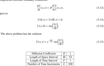
∂U

∂t (x,t)= D

∂2_U

∂x2(x,t), (3.12)

subject to:

U(0,t)= U( ˜M,t)= 0, (3.13)

U(x,0)= sin πx ˜

M

!

. (3.14)

The above problem has the solution:

U(x,t)=e−Dπ 2_t ˜

M2 _sin πx

˜

M

!

. (3.15)

Diffusion Coefficient D 1₂

Length of Space Interval M˜ 10 Length of Time Interval T 1 Number of Time Increments L˜ 100

Table 3.1: Parameters used in the implementation of the Crank-Nicolson numerical scheme for the one-dimensional heat equation.

(38)

0 2 4 6 8 10 0 0.1 0.2 0.3 0.4 0.5 0.6 0.7 0.8 0.9 1 x U(x,t)

0 2 4 6 8 10

0 0.1 0.2 0.3 0.4 0.5 0.6 0.7 0.8 0.9

1x 10

−6

x

Absolute Error

True Solution Numerical Solution

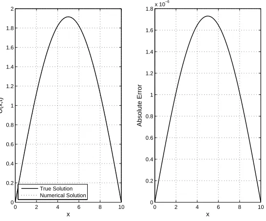
Figure 3.1: Comparison of the numerical and true solution for one-dimensional heat equation at timet=1. All parameters as given in Table 3.1.

3.3 Application to the Black-Scholes PDE

Recall the Black-Scholes pricing partial differential equation for a general option with price

U(S, τ), written on an underlying asset following geometric Brownian motion with constant drift and volatility. Our space variable is now the stock price variable S. Recall that we reversed time usingτ=T −t, thus our pricing PDE is:

∂U

∂τ(S, τ)=

1 2σ

2 S2∂

2_U

∂S2(S, τ)+rS

∂U

∂S (S, τ)−rU(S, τ). (3.16)

The initial and boundary conditions depend on the type of option contract. We will assume they are defined for the implementation of numerical methods.

We first need to replace our partial derivatives embedded in our pricing PDE with finite difference approximations. We assume that our time increment is given by dτ = dt. Then using the fact thatS =mdS wheredS is our stock price increment, our pricing PDE becomes:

Ul+1

m −U l m dt = 1 2 (" 1 2σ

2₍_mdS₎2 U

l

m+1−2U

l m+U

l m−1 dS2

!

+rmdS U l

m+1−U

l m−1

2dS

! −rU_ml

# + " 1 2σ 2

(mdS)2 U

l+1

m+1−2U

l+1

m +U l+1

m−1 dS2

!

+rmdS U l+1

m+1−U

l+1

m−1

2dS

!

−rUml+1 #)

,

Options Pricing and Hedging in a Regime-Switching Volatility Model

Scholarship@Western

Scholarship@Western

Options Pricing and Hedging in a Regime-Switching Volatility

Options Pricing and Hedging in a Regime-Switching Volatility

Model

Model

VOLATILITY MODEL

(Thesis format: Monograph)

by

Melissa Anne Mielkie

Graduate Program in Applied Mathematics

A thesis submitted in partial fulfillment

of the requirements for the degree of

Doctor of Philosophy

The School of Graduate and Postdoctoral Studies

The University of Western Ontario

London, Ontario, Canada

c

Abstract

Contents

List of Figures

List of Tables

List of Appendices

List of Abbreviations and Symbols

List of Abbreviations

List of Symbols

Chapter 1

Introduction

Chapter 2

Regime-Switching Framework

2.1

Market Assumptions

2.2

Geometric Brownian Motion

2.3

N

-State Case

2.3.1

Regime-Switching Volatility

2.3.2

Regime-Switching Option Dynamics

2.3.3

Pricing Equation Derivation

2.4

Two-State Case

Chapter 3

Numerical Solution

3.1

Overview of Crank-Nicolson Numerical Scheme

3.2

Application to the One-Dimensional Heat Equation

3.3

Application to the Black-Scholes PDE