Electronic Thesis and Dissertation Repository
7-28-2011 12:00 AM
FEM-FCT Based Dynamic Simulation of Trichel Pulse Corona
FEM-FCT Based Dynamic Simulation of Trichel Pulse Corona
Discharge in Point-Plane Configuration
Discharge in Point-Plane Configuration
Paria Sattari
The University of Western Ontario Supervisor
Dr. K. Adamiak
The University of Western Ontario Joint Supervisor Dr. G.S.P. Castle
The University of Western Ontario
Graduate Program in Electrical and Computer Engineering
A thesis submitted in partial fulfillment of the requirements for the degree in Doctor of Philosophy
© Paria Sattari 2011
Follow this and additional works at: https://ir.lib.uwo.ca/etd
Part of the Electromagnetics and Photonics Commons
Recommended Citation Recommended Citation
Sattari, Paria, "FEM-FCT Based Dynamic Simulation of Trichel Pulse Corona Discharge in Point-Plane Configuration" (2011). Electronic Thesis and Dissertation Repository. 215.
https://ir.lib.uwo.ca/etd/215
This Dissertation/Thesis is brought to you for free and open access by Scholarship@Western. It has been accepted for inclusion in Electronic Thesis and Dissertation Repository by an authorized administrator of
SIMULATION OF TRICHEL PULSE
CORONA DISCHARGE IN
POINT-PLANE CONFIGURATION
(Spine title: Numerical Simulation of Trichel Pulse Corona Discharge) (Thesis format: Monograph)
by
Paria Sattari
Graduate Program in Engineering Science Department of Electrical and Computer Engineering
A thesis submitted in partial fulllment of the requirements for the degree of
Doctor of Philosophy
School of Graduate and Postdoctoral Studies The University of Western Ontario
London, Ontario, Canada July, 2011
c
THE UNIVERSITY OF WESTERN ONTARIO
SCHOOL OF GRADUATE AND POSTDOCTORAL STUDIES
Chief Advisors: Examining Board:
Dr. Kazimierz Adamiak Dr. Anestis Dounavis
Dr. G. S. Peter Castle Dr. Wamadeva Balachandran
Advisory Committee: Dr. William D. Greason
Dr. Dimitre Karamanev
The thesis by Paria Sattari
entitled:
FEM-FCT BASED DYNAMIC SIMULATION OF TRICHEL PULSE CORONA DISCHARGE IN POINT-PLANE CONFIGURATION
is accepted in partial fulllment of the requirements for the degree of
Doctor of Philosophy
Date:
Chair of Examining Board
In this thesis, a new two-dimensional numerical solver is presented for the dynamic simulation of the Trichel pulse regime of negative corona discharge in point-plane con-guration. The goal of this thesis is to simulate the corona discharge phenomenon and to improve existing models so that the results have an acceptable compatibility with the experimentally obtained data. The numerical technique used in this thesis is a combination of Finite Element Method (FEM) and Flux Corrected Transport (FCT). These techniques are proved to be the best techniques, presented so far for solving the nonlinear hyperbolic equations that simulate corona discharge phenomenon.
The simulation begins with the single-species corona discharge model and the dierent steps of the numerical technique are tested for this simplied model. The ability of the technique to model the expected physical behaviour of ions and electric eld is investigated. Then, the technique is applied to a more complicated model of corona discharge, a three-specie model, in which three ionic species exist in the air gap: electrons, and positive and negative oxygen ions. Avalanche ionization, electron attachment and ionic recombination are the three ionic reactions which this model includes.
The macroscopic parameters i.e., the average corona current and the Trichel pulses period are calculated and compared with the available experimental data. The technique proves to be compatible with the available experimental results. Finally, the eects of dierent parameters on the Trichel pulse characteristics are investigated. The results are further compared against the available experimental data for the eect of pressure on Trichel pulse characteristics and are reported to be compatible.
Keywords: negative electric corona discharge, Trichel pulse, nite element method, ux corrected transport, numerical simulation.
I would like to give my best regards and gratefulness to Prof. K. Adamiak. Without his consistent help, support, and guidance, I would have been lost in the middle of this project.
Secondly, I would like to thank Prof. G.S.P Castle for his invaluable comments during the course of this project. His great insight and profound knowledge was of great help for me.
I also like to acknowledge the helpful discussions and advises of C.F. Gallo and Dr. P. Atten at dierent stages of my project.
I would also like to thank Mr. Dan Sich from the library, who helped me nd many papers. My thanks to Mr. B. Saunders and Mr. T. Hunt for their help with Linux operating systems and the SHARCNET of Canada for the resources they provided for my computational analysis.
I am grateful to NSERC of Canada and UWO for their nancial support. I also acknowledge and admire my colleagues for helping me during the course of this project.
Last but not least, I take this opportunity to thank my husband, Nima, and my parents, for their unconditional love and support they gave me during these years.
To my family;
Nima, Roohangiz, Siavash, Pegah, and Sara
Certicate of Examination . . . ii
Abstract . . . iii
Acknowledgements . . . iv
Dedication . . . v
List of Figures . . . x
List of Tables . . . xiv
Acronyms . . . xv
Nomenclature . . . xvii
1 Introduction . . . 1
1.1 What is Corona Discharge? . . . 1
1.2 Features of Corona Discharge . . . 2
1.3 Types of Corona Discharge . . . 4
1.4 Mechanism of Negative and Positive corona . . . 4
1.5 Thesis Objectives . . . 6
1.6 Thesis Outline . . . 9
2.1 Mechanism of Trichel Pulse Corona Discharge . . . 12
2.2 Ionic Reactions . . . 17
2.2.1 Ionization . . . 18
2.2.2 Attachment . . . 18
2.2.3 Detachment . . . 19
2.2.4 Ionic Recombination . . . 19
2.2.5 Ozone Generation and Decomposition . . . 20
2.3 Literature Review . . . 21
2.4 Motivation . . . 25
2.5 Conclusions . . . 26
3 Mathematical Models and Numerical Algorithms in Electric Corona Simulation . . . 28
3.1 Introduction . . . 28
3.2 Literature Review on Mathematical Models for the Trichel Pulse Sim-ulation . . . 29
3.3 Literature Review on the Numerical Techniques . . . 30
3.3.1 Numerical Techniques for Calculating the Electric Field . . . . 31
3.3.2 Numerical Methods for Calculating the Space Charge Density 34 3.3.3 Numerical Algorithms for the Simulation of Corona Discharge 36 3.4 Why FEM-FCT? . . . 41
3.5 Finite Element Method . . . 43
3.6 Combined FEM-FCT . . . 48
3.7 Conclusions . . . 54
4 Implementation of FEM-FCT Algorithm for Trichel Pulse Simula-tion . . . 55
4.1 Governing Equations . . . 55
4.2 Implementation of the Numerical Algorithm . . . 61
4.3 Optimization Techniques . . . 65
4.4 Conclusions . . . 67
5.1 Introduction . . . 69
5.2 Mathematical Model . . . 70
5.2.1 Governing Equations . . . 70
5.2.2 Boundary Conditions . . . 71
5.3 Results . . . 75
5.3.1 Step Voltage . . . 75
5.3.2 Pulse Voltage . . . 79
5.4 Conclusions . . . 87
6 Two dimensional Simulation of Trichel Pulses in Air . . . 89
6.1 Introduction . . . 89
6.2 Basic Equations . . . 90
6.3 Boundary Conditions . . . 91
6.4 Numerical Algorithm . . . 92
6.5 Current Components . . . 94
6.6 Results . . . 96
6.6.1 Applied Voltage = -8kV . . . 97
6.6.2 Applied Voltage = -10kV . . . 103
6.7 Conclusions . . . 107
7 A Parametric Study on Trichel Pulse Characteristics . . . 108
7.1 Introduction . . . 108
7.2 Eect of Dierent Parameters on Trichel Pulse Characteristics . . . . 109
7.2.1 External Resistance . . . 109
7.2.2 Ion Mobility . . . 111
7.2.3 Secondary Electron Emission Coecient . . . 117
7.3 Spatial Distribution of Ionic Species in Air Gap . . . 118
7.4 Shape of Ionization Layer . . . 119
7.5 Conclusions . . . 121
8.1 Introduction . . . 125
8.2 Comparison With Gallo's Experimental Data . . . 126
8.3 Appearance and Physics of the Trichel Pulse Near Needle Tip . . . . 128
8.4 Revised Comparison With Gallo's Experimental Data . . . 131
8.5 Eect of Pressure on Trichel Pulse Characteristics . . . 132
8.6 Comparison with Atten's Experimental Data . . . 133
8.7 Conclusions . . . 135
9 Modelling of Corona Discharge in Oxygen . . . 136
9.1 Introduction . . . 136
9.2 Databases . . . 137
9.3 Available Discharge Models . . . 137
9.3.1 Morrow's Model [30] . . . 140
9.3.2 Eliasson et al. Model [23] . . . 140
9.4 Results . . . 143
10 Summary, Conclusions and Recommendations for Future Study . 152 10.1 Summary . . . 152
10.1.1 Dynamic Single-Species Model of Corona Discharge . . . 152
10.1.2 Simulation of Trichel Pulse in Air . . . 153
10.1.3 Parametric Study of Trichel Pulse Characteristics . . . 154
10.1.4 Experimental Verication of the Numerical Results . . . 154
10.1.5 Trichel Pulse Simulation in Oxygen . . . 154
10.2 Conclusions . . . 155
10.3 Recommendations for Future Study . . . 157
Appendices A Appendix A . . . 172
A.1 Oxygen Model Databases . . . 172
B Curriculum Vitae . . . 178
1.1 Types of positive corona discharge, from left: burst corona, glow corona,
streamer corona, spark discharge. . . 6
1.2 Types of negative corona discharge, from left: Trichel pulse corona, pulseless corona, spark. . . 7
2.1 Ionic reactions in corona discharge. The scaling is not accurate. . . . 15
2.2 Electric eld in dierent regions during Trichel pulse corona discharge, the circles represents the ion clouds. . . 16
4.1 The conguration of corona discharge system. . . 56
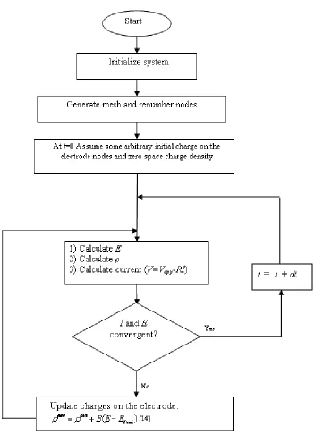
5.1 Flowchart of the simulation process. . . 76
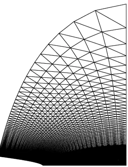
5.2 FE grid used in the simulation process. . . 77
5.3 Corona current versus time (Rext = 50MΩ, V = 10kV) . . . 78
5.4 Corona current versus time for two dierent external resistances (V=10kV). 79 5.5 Current versus time for two dierent input voltages (Rext = 5MΩ). . 80
5.6 Space charge density along the axis of symmetry at six dierent instants of time (Rext = 50MΩ). . . 80
5.7 Applied pulse voltage described by Vs(t) = Vtmmte(1− t tm)+VDC. . . . 81
5.8 Corona current versus time for the pulse voltage shown in Figure 5.7 (Rext = 50MΩ). . . 82
5.9 Space charge density on the tip of the corona point versus time for the pulse voltage (Rext = 50MΩ). . . 82
5.10 Charge density along the axis for ve dierent time instants after the rst voltage pulse (Rext= 50MΩ). . . 83
5.11 Charge distribution in the space for a pulse energization at t=10 µs (Rext = 50MΩ). . . 84
5.12 Charge distribution in the space for a pulse energization at t=210 µs (Rext = 50MΩ). . . 84
Rext = 50MΩ) . . . 85
5.14 Corona current versus time for a pulse energization, (f = 50kHz, Rext = 50MΩ) . . . 86
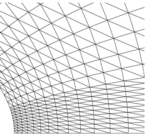
5.15 Charge distribution in the space between both electrodes at t=41 µs . 86 6.1 Details of FE grid near corona electrode used in the simulation process. 94 6.2 Circuit model of the needle-plane conguration. . . 96
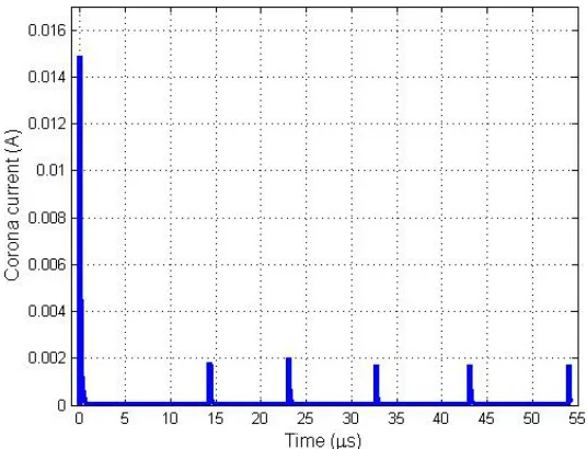
6.3 Corona current for V = -8kV. . . 98
6.4 Displacement current for V = -8kV. . . 99
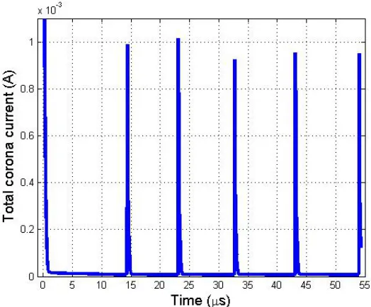
6.5 Total current for V = -8kV, the amplitude of the rst pulse is approx-imately equal to the amplitude of the displacement current at t=0. . 99
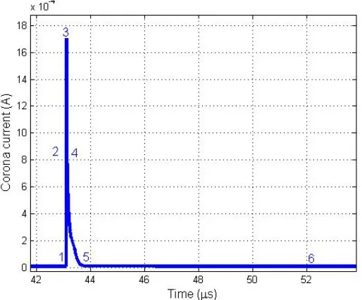
6.6 Characteristic points on a typical Trichel pulse: 1 - beginning of the pulse, 2 - half-pulse rising, 3 - maximum of the pulse, 4 - half-pulse decreasing, 5 - end of the pulse, 6 -9 microseconds after the pulse . . 100
6.7 Electron density along the axis of symmetry at dierent instants during a Trichel pulse (In gures 6.7, 6.8 and 6.9, the minimum scale on y axis is chosen to be 0.0001 and the values below this level are considered as noise. Therefore the curves which do not exist in these gures are in the noise level). . . 101
6.8 Positive ion density along the axis of symmetry at dierent instants during a Trichel pulse. . . 102
6.9 Negative ion density along the axis of symmetry at dierent instants during a Trichel pulse. . . 102
6.10 Electric eld along the axis of symmetry at dierent instants during a Trichel pulse. . . 104
6.11 Trichel pulse for V=-10kV. . . 105
6.12 Total electron charge in the air gap versus time. . . 105
6.13 Total negative ion charge in the air gap versus time. . . 106
6.14 Total positive ion charge in the air gap versus time. . . 106
7.1 Trichel pulse period versus applied voltage for dierent external resis-tances . . . 112
7.2 Average corona current versus applied voltage for dierent external resistances . . . 112
7.4 Total charge of positive ions versus time (Rext = 100kΩ) . . . 113
7.5 Total charge of electrons versus time (Rext = 10kΩ) . . . 114
7.6 Total charge of electrons versus time (Rext = 100kΩ) . . . 114
7.7 Total charge of negative ions versus time (Rext= 10kΩ) . . . 115
7.8 Total charge of negative ions versus time (Rext= 100kΩ) . . . 115
7.9 Total corona current versus time (Rext= 10kΩ) . . . 116
7.10 Total corona current versus time (Rext= 100kΩ) . . . 116
7.11 Trichel pulse period versus secondary electron emission coecient . . 118
7.12 Average corona current versus secondary electron emission coecient 119 7.13 Positive ion density at point P1 . . . 120
7.14 Electron density at point P1 . . . 120
7.15 Negative ion density at point P1 . . . 121
7.16 Trichel pulses for V=-9kV . . . 122
7.17 The thickness of the ionization layer . . . 122
7.18 Electric eld on the tip of corona electrode . . . 123
7.19 Ionization prole at dierent instants of time . . . 123
8.1 Trichel pulse period versus applied voltage - comparison of experimen-tal and numerical results . . . 127
8.2 Average corona current versus applied voltage: experimental and nu-merical results . . . 128
8.3 Experimental shape of the discharge region . . . 130
8.4 Qi/Qfor V = -9 kV . . . 134
9.1 Mobility of electrons versus the reduced electric eld . . . 138
9.2 Diusion coecient versus the reduced electric eld . . . 138
9.3 Ionization frequency versus the reduced electric eld . . . 139
9.4 Attachment frequency versus the reduced electric eld . . . 139
9.5 Mobility of electrons versus the reduced electric eld . . . 143
9.6 Diusion coecient versus the reduced electric eld . . . 144
9.7 Ionization coecient versus the reduced electric eld . . . 144
9.8 Attachment coecient versus the reduced electric eld . . . 145
9.9 Corona current versus time in oxygen . . . 147
9.12 Total charge of electrons versus time in air . . . 148
9.13 Total charge of positive ions versus time in oxygen . . . 149
9.14 Total charge of positive ions versus time in air . . . 149
9.15 Total charge of negative ions versus time in oxygen . . . 150
9.16 Total charge of negative ions versus time in air . . . 150
9.17 Electric eld versus time in oxygen . . . 151
9.18 Electric eld versus time in air . . . 151
1.1 Corona discharge classication . . . 6
3.1 A comparison between dierential-based and integral-base techniques 31 7.1 Trichel pulse characteristics for dierent applied voltages, Rext = 100 kΩ . . . 111
7.2 Trichel pulse characteristics for dierent applied voltages, Rext = 50 kΩ111 7.3 Trichel pulse characteristics for dierent applied voltages, Rext = 10 kΩ111 7.4 Trichel pulse characteristics for V =−7kV and dierent ion mobilities 117 7.5 Trichel pulse characteristics for dierent secondary emission coe-cients, V =−7kV . . . 118
8.1 Rough estimates of dimensions . . . 130
8.2 Trichel pulse characteristics for V =−4kV, r= 10µm, d= 6mm . . . 132
8.3 Trichel pulse period and pulse duration versus gas pressure (V=-9kV, Rext=100 kΩ) . . . 133
8.4 Charge-per-pulse (in picocoulombs) for two congurations with dier-ent radii . . . 134
9.1 Morrow's model coecients [30] . . . 141
9.2 Eliasson et al. model coecients based on Zhang et al. [100] . . . 142
A.1 Model coecients in oxygen: Siglo database . . . 173
A.2 Model coecients in oxygen: Morgan database . . . 174
A.3 Model coecients in oxygen: Phelps database . . . 175
A.4 Mobility of positive ions . . . 176
A.5 Mobility of negative ions . . . 177
AC Alternating Current
BEM Boundary Element Method
CFD Computational Fluid Dynamics
CSM Charge Simulation Method
DC Direct Current
DCM Donor Cell Method
ESP Electrostatic Precipitator
FCT Flux Corrected Transport
FDM Finite Dierence Method
FEM Finite Element Method
FVM Finite Volume Method
MoC Method of Characteristics
MoM Method of Moment
ODE Ordinary Dierential Equations
1D One Dimensional
2D Two Dimensional
3D Three Dimensional
3S Three Species
⃗
A Vector Magnetic Potential (V.s.m−1) ⃗
B Magnetic Field Intensity (Tesla)
⃗
D Electrostatic Displacement (C.m−2)
D Diusion Coecient (m2.s−1)
Eo Onset Value of Electric Field (V.m−1) EP eek Peek's Value (V.m−1)
e0 Electron Charge (C)
⃗
E Electric Field Intensity (V.m−1)
EN Reduced Electric Field (Td)
f Frequency (Hz)
I Corona current (A)
Id Displacement Current (A)
Itot Total Current (A)
⃗j Electric Current Density (A.m−2)
k Mobility of Charge Carriers (m2.V−1.s−1) ki Ionization Frequency (s−1)
ka Attachment Frequency (s−1)
kd Detachment Frequency (s−1)
kb Boltzmann Constant (m2.kg.s−2.K−1) µe Mobility of Electrons (m2.V−1.s−1) µn Mobility of Negative Ions (m2.V−1.s−1) µp Mobility of Positive Ions (m2.V−1.s−1) Ne Number Density of Electrons (m−3) Nn Number Density of Negative Ions (m−3) Np Number Density of Positive Ions (m−3) N O2 Concentration of Oxygen Molecules (m−3)
P Pressure (atm)
P0 Standard Pressure (atm)
req Electrode Equivalent Radius (m)
Rext External Resistance (Ω)
t Time (s)
∆t Time Step (s)
T Absolute Temperature (K)
T0 Standard Temperature (K)
⃗
u Velocity of the Ions (m.s−1)
V Electric Potential (V)
V0 Corona Onset Voltage (V)
⃗
We Drift Velocity of Electrons (m.s−1) ⃗
Wn Drift Velocity of Negative Ions (m.s−1) ⃗
Wp Drift Velocity of Positive Ions (m.s−1)
ε0 Gas Permittivity (F.m−1)
βep Electron-Ion Recombination Coecient (m3.s−1) βnp Ion-Ion Recombination Coecient (m3.s−1)
γ Secondary Electron Emission Coecient
α Ionization Coecient (m−1)
η Attachment Coecient (m−1)
Chapter 1
Introduction
1.1 What is Corona Discharge?
Corona is a partial discharge phenomenon that requires at least two electrodes: a sharp electrode with very small radius of curvature, usually supplied with a high electric potential which is called the corona electrode and a blunt electrode with much larger radius of curvature which is usually grounded. The partial electrical discharge, which occurs when the strength of the electric eld near the corona electrode exceeds a certain critical value but still insucient for a complete breakdown or arc is known as the electric corona discharge. In corona systems, the electric eld near the sharp corona electrode has to be much larger than its value at points far from this electrode. Therefore, in contrast to a spark discharge, only a very small part of the gap between the two electrodes becomes ionized and conductive during the discharge; this is why corona is a called a partial discharge phenomenon.
nine orders of magnitude during a few nanoseconds [1].
Corona electrodes typically consist of needles (points), wires or blades connected to a high voltage power supply [2]. Some examples of dierent congurations used for generating corona discharge are point-to-plane, multi-point-to-plane, wire-to-plane, wire-to-cylinder, wire between two planes, and multi-wire-to-plane [3]-[5].
1.2 Features of Corona Discharge
The value of the potential at which corona starts is called the corona threshold or the corona onset voltage. At voltages close to this value, there is a region in which corona current increases proportionally with voltage. This region is called the Ohm's law regime. Above this region, the corona current increases more rapidly, approximately as a square function of the applied voltage. Increasing the applied voltage eventually leads to a complete breakdown and arcing at a point called the breakdown potential.
characteristics of the gas and the size and surface condition of the high voltage elec-trode. Peek [6] obtained an expression for the value of critical electric eld, at which corona discharge starts on a corona electrode in dry air for highly symmetric cong-urations.
For over a hundred years the corona discharge has been used in industry. Since electrostatic processes often depend on availability of charge carriers [7], the main application of corona discharge in engineering devices and processes involves the electrical charging of small particles or drops [8]. Examples of devices using this phenomenon include the electrostatic precipitator of Cottrell [9], electrophotography, powder coating systems, static control in semiconductor manufacture, ionization in-strumentation, control of acid gases from combustion sources, destruction of toxic compounds, generation of ozone [10], reduction of gaseous pollutants SOx and N Ox in ue gases [11], jet printers, indoor air cleaners, and industrial processes such as the treatment of polymer lms and fabrics [12].
1.3 Types of Corona Discharge
Corona discharge phenomena can be categorized from dierent points of view:
1. Discharge current: burst pulse corona, streamer corona, Trichel pulse corona and glow corona. The specications and characteristics of these regimes are described later in this Chapter.
2. Electrode conguration: electrode conguration has a major role in dierent applications of corona discharge. For example, in coating technology, where a high homogeneity is needed, point-plane conguration is used. In gas and water treatment applications, dierent congurations such as wire, wire-plane, wire-cylinder and mesh/brush congurations have been investigated and implemented on industrial scales [13].
3. Polarity of the electric potential supplied to a sharp electrode: negative corona and positive corona.
In negative corona, a negative voltage is applied to the corona electrode. Elec-trons and negative ions move towards the ground plane and positive ions move towards the corona electrode. Trichel pulses only happen in negative corona and will be explained in detail in Chapter 2. In positive corona on the other hand, the applied voltage and the direction of ions movement is opposite to that of the negative corona case.
1.4 Mechanism of Negative and Positive corona
with short and faint streamers away from the needle [14]. It then proceeds to the glow corona, streamer corona and nally spark discharge as the applied voltage increases [10]. The positive glow corona is known as the Hermstein glow [15]. This glow has a stable current at a xed voltage, quiet operation and almost no sparking. The streamer regime is unstable, and emits audio and radio noise. It creates many thin and short duration current streamers originating from the needle. This behaviour is shown in Figure 1.1 as a brush growing [14]. The streamer regime of corona can be described as an incomplete breakdown and it is followed by a spark as voltage is increased further [10]. For a wire-cylinder or wire-plate electrode conguration, corona generated at a positive wire electrode may appear as a tight sheath around the electrode or as a streamer moving away from dierent parts of the electrode [10].
Polarity of the electric eld Positive Negative Discharge current Burst pulse corona
Streamer corona Glow corona
Spark
Trichel pulse corona Pulseless corona
Spark
Electrode conguration Point to plate, Wire to plate, Wire to cylinder
potential in comparison to the positive corona; this is why negative corona is often used in electrostatic precipitators [14].
The classication of corona discharge from these dierent point of views is shown in Table 1.1.
Figures 1.1 and 1.2 show dierent types of corona discharge from the discharge current point of view [17].
Figure 1.1: Types of positive corona discharge, from left: burst corona, glow corona, streamer corona, spark discharge.
1.5 Thesis Objectives
Figure 1.2: Types of negative corona discharge, from left: Trichel pulse corona, pulseless corona, spark.
particular interest is what happens to the magnitude and distribution of the electric eld and charge species during this process and how they behave. This technique should be able to produce results compatible with available experimental data. The main objectives of this thesis are as follows:
To present an applicable model for simulating the Trichel Pulse phe-nomenon found in negative corona discharge in point-to-plane congura-tion in oxygen and air:
single-Therefore, presenting a model which can accurately predict the physical behaviour of corona discharge has still been missing. In this thesis, a dynamic, three-species, 2D model for predicting the mechanism of the Trichel pulse regime of corona discharge is presented.
To present a numerical technique for solving the model:
The corona discharge is a very complicated phenomenon for which an analytic solution is not available. Also, the governing equations for modelling the behaviour of charge carriers are not easily solvable. Therefore, presenting a technique which can deal with the nonlinear hyperbolic equations modelling this problem is very desirable. To date, many numerical techniques have been presented for solving the hyperbolic equations of charge transport. Of these a combined Finite-Element-Method (FEM) and Flux Corrected Transport (FCT) technique has proved to be the best one for dealing with these classes of problems. However, numerical implementation of this technique is very complicated and needs some modications for a specic type of problem. In this thesis, a FEM method is used for solving the Poisson equation and a combined FEM-FCT technique is proposed for solving the charge transport equations.
To compare the simulation results with the experimental data:
of Trichel pulse corona in air, the most complete 2D dynamic model is chosen; a numerical technique is developed for solving this model and the numerical predictions are compared with the available experimental data presented by other researchers.
To investigate the eect of dierent parameters of the model on the corona characteristics:
Some of the parameters used in modelling negative corona discharge dier widely in the literature and various values are used in dierent papers. Since knowing the eect of these parameters on the Trichel pulse characteristics is important, the eect of parameters such as external resistance, mobility, air pressure, and the sec-ondary electron emission coecient are investigated in this thesis and the observations are reported.
1.6 Thesis Outline
This thesis is divided into eight Chapters. A summary of each Chapter follows.
Chapter 2: This Chapter focuses on explaining the mechanism of negative corona discharge in Trichel pulse regime. It also reviews the literature related to the Trichel pulse regime of corona discharge, mentions the deciencies of these mod-els and explains the motivation of this work.
are explained in detail. FEM is used for the electric eld computations and the FEM-FCT technique is used for the space charge density calculations.
Chapter 4: In this Chapter, the complete set of equations for modelling the Trichel pulse regime of corona discharge is presented and the solution methodology is explained. Moreover, the numerical problems faced during the course of this work are presented. The suggested solutions for these problems are presented along with several techniques used for optimizing the code.
Chapter 5: In this Chapter, a numerical algorithm for the dynamic simulation of corona discharge in air, assuming single species charge carriers is proposed. The simulation results show the behaviour of corona current and space charge density under two waveforms of the applied voltage: step and pulse.
Chapter 6: In this Chapter, which is the main Chapter of this thesis, Trichel pulses are numerically reproduced. The mechanism of these pulses is explained by discussing in detail eld and charge behaviour during these pulses. It is assumed that three ionic species exist in the air gap: electrons, and positive and negative oxygen ions.
Chapter 7: In this Chapter, eects of dierent parameters of the model on Trichel pulse characteristics (i.e., Trichel pulse period and the average corona current) are studied. The parameters of interest are: external resistance of the circuit, secondary electron emission coecient, and negative and positive ion mobilities.
of corona discharge in oxygen is presented. A series of Trichel pulses are simu-lated in oxygen as well.
Chapter 2
Negative Corona Discharge
2.1 Mechanism of Trichel Pulse Corona Discharge
Electronegative gases are gases which have anity for electrons. These gases are characterized by one or two electrons decient in their outer shell [18]. Oxygen, water vapour, and carbon dioxide are several common examples for electronegative gases [12]. The gases that do not have the anity for electrons are called free-electron gases [18]. Nitrogen, hydrogen, helium, and argon are several examples of free-electron gases.
onset voltage1, a very large electric eld appears near the corona electrode. If this electric eld exceeds the critical value required for the ionization of the gas, the corona discharge is initiated. The threshold value for the electric eld depends on factors such as wire radius, the roughness of the wire, ambient gas temperature and pressure [12].
In the area between electrodes there are always some seed electrons (20 electron-ion pairs/cm3 per second at atmospheric pressure) which are created due to cosmic
radiations and other phenomena. When the electric eld is large enough, these seed electrons are accelerated and upon colliding with neutral molecules, detach electrons from these molecules leaving positive oxygen ions. In a very short time a very large number of electrons and positive ions is created in the ionization layer2. This process is called avalanche ionization.
Since beyond the ionization layer electrons do not have enough energy to detach electrons from the neutral molecules, this process stops at the edge of the ionization layer.
Free electrons may also attach to neutral molecules of the electronegative gas and create negative ions. This attachment process happens in both the ionization and drift region3. Recombination between positive ions and electrons or between
1. The voltage at which the electric eld on the corona electrode is equal to the Peek's value
2. The region in which the electric eld can accelerate electrons to the speed at which they can detach electrons from the neutral molecules
air gap. Recombination results in the reduction of the number of ions and electrons. The secondary electrons which sustain the discharge have three dierent sources: photoemission from the discharge electrode, collision of positive ions with the corona electrode surface and photoionization in the gas [21].
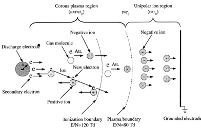
There are two distinct regions in the corona discharge [22]. In the vicinity of the corona electrode, in which avalanche ionization occurs due to the collision of highly accelerated electrons with neutral molecules, an ionization layer exists. In most cases, this layer is less than a few millimetres around the electrode [22]. A larger region which is called the drift region is the region which is mostly lled with ions of the same polarity as those of the corona electrode. In the ionization layer, ionization prevails over attachment. Beyond the ionization layer the electric eld decreases gradually and electrons do not have sucient energy to ionize the gas molecules. Therefore, the avalanche ionization stops and the number of electrons decrease gradually in the drift region. Since beyond the ionization layer and in the drift region, there might be some electrons with sucient energy for the ionization of gas molecules, some authors assume another layer, called the plasma layer, which is a region starting from ionization boundary and extends a few milimeters into a drift region. Davidson [12] has dened this region as the corona plasma region, in which corona-enhanced chemical reactions are possible and its radius is the radius at which the reduced eld
E/N (where N is the density of neutral molecules) equals 80 Td. At this value the
Figure 2.1: Ionic reactions in corona discharge. The scaling is not accurate.
Subsequent to the avalanche ionization, a cloud of positive ions is created close to the corona electrode in the air gap. In a very short time, the attachment also creates a cloud of negative ions just outside the ionization layer. This formation of ionic clouds causes the increase of electric eld between the positive ion cloud and the corona electrode, decrease of electric eld between the two clouds and increase of electric eld between the negative ion cloud and the plane as shown in Figure 2.2.
Figure 2.2: Electric eld in dierent regions during Trichel pulse corona discharge, the circles represents the ion clouds.
corona electrode starts, the corona current's value decreases.
The maximum of corona current occurs when the total number of positive ions in the space is largest. At this moment the avalanche ionization has not stopped yet. For a short time after the maximum of the pulse, avalanche ionization still occurs. Therefore, the total number of electrons in the space still increases after the Trichel pulse. However, since the positive ions are being deposited on the corona electrode and the deposition rate is larger than the generation rate, the number of positive ions decreases with time.
are being deposited there. Since the mobility of negative ions is small and they have a long distance to travel (in contrast with positive ions), this deposition process is very slow and takes a long time (in comparison to the rise time of the Trichel pulse). As soon as negative ions start being deposited on the ground, the total number of negative ions in the air gap decreases. Once enough negative ions are deposited on the ground plate and they disappear from the space, the electric eld near the corona electrode increases again and everything gets ready for the next pulse to appear. Right before the next pulse, the secondary electron emission creates a sucient amount of electrons required for the avalanche ionization of the second pulse.
In wire-plate or wire-cylinder congurations, negative corona appears in a form of discrete tufts or beads along the wire [10]. These tufts are randomly spaced along the wire and their number is dependent on the applied voltage. As the voltage increases, the number of tufts increases too and they become more uniformly spaced [12].
2.2 Ionic Reactions
2.2.1 Ionization
In gas discharge, ionization is dened as the process of liberating an electron from a gas particle with either the simultaneous production of a positive ion or with the increase of positive ion charge [18]. There are various ways for the creation of positive ions:
• Electron collision
• positive ion collision
• radiation: light, X-ray, nuclear
• thermal ionization
• excited atoms
• chemical and nuclear processes
Some equations that show the ionization process in oxygen are shown below:
e+O→O++ 2e
e+O2 →O++O+ 2e
e+O3 →O3++ 2e
2.2.2 Attachment
the formation of negative ions is called attachment. Here are some examples for attachment in oxygen:
e+O2 →O−+O e+O+O2 →O−+O2
e+O3 →O−+O2
2.2.3 Detachment
The process of detaching electron from neutral molecules or negative ions is called detachment. Some examples for this process are:
e+O−→O+ 2e
O−+O2 →O+O2+ 2e O−+O →O2+e
2.2.4 Ionic Recombination
Recombination or neutralization is the combination of a positive ion with either a free electron or an excessive electron of a negative ion. This process is a major cause of the decrease in charged particle numbers.
examples for recombination processes:
O−+O2+ →O+O2
O−+O2++O2 →O3 +O2 O++O2−+O2 →O3 +O2
2.2.5 Ozone Generation and Decomposition
Disinfection, bleaching and chemistry are three domains in which ozone has expand-ing applications. In water purication applications, ozone is used extensively as a substitute for chlorine. Electric corona discharge is the best technique for creating ozone. This technique has been investigated for a long time and is now largely indus-trialized. The following equations show the processes causing ozone generation and decomposition in oxygen.
O+O2+O2 →O3+O2
e+O3 →O+O2+e
O3+O2 →O+O2+O2
O3+O →2O2
As mentioned earlier, including all these species and reactions makes the corona model too complicated. Therefore, considering the specic application of corona and the information needed, only some of these species should be considered in the model.
If the charge density distribution of electrons and negative and positive oxygen ions are required, the three species model which only includes the reactions between
e, O2+, O2− should be studied. This model is also sucient for the reproduction of
the reactions between e, O2+, O2−, O3, O should be investigated.
2.3 Literature Review
The Trichel pulse regime of corona discharge which is the rst regime in negative corona is an interesting phenomena from both scientic and industrial points of view. Trichel pulses are normally very regular pulses with very short rise times (as short as 1.3 ns [24]) and short durations (tens of nanoseconds [25]) separated by much longer inter-pulse periods (tens of microseconds [25]). Trichel reported the existence of such pulses in oxygen [16] and was able to explain some very important features of the corona discharge like the shielding eect produced by the positive ion cloud near the cathode. He also predicted that the space charge formation and subsequent clearing in the gap is the cause of the periodic character of the discharge. A negative cloud of space charge is formed far from the discharge electrode (point) and a positive cloud is formed near the point. The presence of positive ions near the point increases the eld in this area and decreases the electric eld between the positive and the negative ion clouds. Therefore, no ionization can take place beyond the positive ion cloud. The positive ions move towards the point under the eect of the electric force; this narrows the region of the enhanced electric eld and, nally, the ionization process stops.
gases. This assumption contradicts the recent discovery of Akishev at al. [19]. They tried to explain this phenomenon by presenting a theory which involved successive electron avalanches, each giving rise to three successors near the end of its develop-ment but this theory could not explain the fast rise time of 1.5ns observed in air at atmospheric pressure.
Zentner 1970 [24] found that the rise time of the pulse in air may be as short as 1.3 ns. He also observed a step on the leading edge of the current pulse.
Lama and Gallo [26] carried out a series of carefully designed experiments and determined the dependence of pulse frequency, charge per pulse and time averaged corona current with the applied voltage, needle tip radius, and needle to plane spacing. They further explained the physical mechanism proposed by Trichel and Loeb, by adding a very rapid electron Townsend avalanche from the tip, followed by electron attachment to electronegative molecules to form a slow moving negative ion cloud that reduces the electric eld below threshold and thus chokes the discharge. The corona discharge then remains o until the negative ion cloud drifts suciently far from the tip causing the electric eld to rise above threshold and the discharge re-initiates. This is repeated in successive stages leading to Trichel current pulses. Lama and Gallo analyzed the electric eld and characterized the discharge in terms of several parameters as follows dened in terms of applied voltage, gap spacing and tip radius:
• Transit time: the time for a negative ion cloud to transverse the gap.
• The number of negative ion charge clouds in the gap at any given time, partic-ularly as a function of applied voltage.
• The total value of negative ion charge in the gap at any given time, particularly as a function of applied voltage.
By incorporating experimental data into the expressions for the charge-free electric eld, Lama and Gallo were able to obtain equations for the complex space-charge perturbed situation. These equations remain to be veried by independent analysis. Depending upon applied voltage, their major conclusion is that there are many negative ion charge clouds simultaneously in transit across the gap.
Aleksondrov [28] presented the theory of parallel development of several avalanches rather than successive avalanches. He therefore succeeded in predicting much faster rise times for the main pulse. Kekez et al. [29] used an equivalent circuit for the point-to-plane corona discharge and described the succession of pulses. However, his model could not explain the detailed mechanism of the pulse formation.
decay of the current without subsequent pulses. Although Morrow did explain the dierent stages of the pulse, he ignored the ion secondary emission.
Atten et al. [32] investigated the process of corona discharge in air at dierent gas pressures and point radii. They showed that the Paschen's law is still valid in high pressure air (up to 7 MPa) for very small point electrodes.
Castellanos et al. [33] proposed a three species model to study corona discharge in oxygen at a reduced pressure (50 Torr). They solved the problem in 1D using a Particle-in-Cell technique. Their results were compared with experimental data, but the model they were using was valid for oxygen and at a reduced pressure while the experimental data was reported for air and at atmospheric pressure [26]. Moreover, the investigated geometry was dierent from that of experiment. Therefore, they did not expect a quantitative agreement between experimental and numerical results. Still their model and technique had some advantages; it was fast and they could obtain a reasonable agreement between the characteristics of Trichel pulse in simulation and experiment.
Napartovich et al. [34] proposed a quasi-one-dimensional, 1.5D, numerical model for the analysis and reproduction of Trichel pulses. This means that they assumed a constant distribution for all the physical quantities (charge densities and electric eld) in every cross section of the discharge channel. The same approximation was made by Morrow but he assumed a cylindrical shape for the discharge channel. However, experimental observations show that the ratio of the discharge channel on the anode and cathode is on the order of 104. They assumed that the radius of the
The same authors later presented a two-dimensional model for negative corona discharge in air and successfully showed the presence of a sequence of Trichel pulses [35]. This paper, however, did not contain any detail on the technique and the model used. Some other authors used similar simplied models in order to reproduce sequences of Trichel pulses [29], [36] and [37].
Georghiou et al. [38] presented a two-dimensional model for Trichel pulse simu-lation in air. They used COMSOL-Multiphysics (a FEM based commercial software) for solving the corresponding equations. Their results, however, were not compati-ble with experimental expectations. The period of the Trichel pulses they calculated was approximately 20 times smaller than the experimental predictions for the same conguration.
2.4 Motivation
for modelling this phenomenon are either comprehensive or compatible with the ex-perimental data. Therefore, a model for simulating Trichel pulse regime of corona discharge will be proposed in this thesis. The proposed model improves the existing models and has the following features simultaneously:
• it is three-dimensional
• it can simulate the dynamic behaviour of Trichel pulses
• it includes three ionic species and it can be easily modied to include a larger number of species
• it is the rst proposed model which shows a reasonable correlation with the experimental data published by other researchers.
2.5 Conclusions
In this chapter, a detailed description of the mechanism of negative corona discharge was presented and the literature related to Trichel pulses was reviewed.
The literature review has identied some specic deciencies in the understand-ing and explanation of Trichel pulses which justies the motivation for this project.
experimental data is certainly a worthy topic of an engineering study.
Chapter 3
Mathematical Models and Numerical
Algorithms in Electric Corona Simulation
3.1 Introduction
Due to the complexity of equations governing corona discharge, nding analytical solutions for these equations is not possible unless some major simplications are made or the problem geometry is highly symmetric. Therefore, numerical simulation is principally the only feasible approach for the corona discharge modelling.
The use of numerical tools for studying this phenomenon has recently reached an advanced degree of development. Dierent types of numerical techniques have been used for modelling this interesting and complicated phenomenon. However, there is still no complete and stable algorithm for modelling the Trichel pulse regime of corona discharge.
equations. The charge density distribution is unknown in advance due to its depen-dence on the electric eld. On the other hand, the eld distribution is a function of charge density. Therefore, the solution of these equations can not be found easily and both problems are mutually coupled.
In order to simulate electric corona discharge numerically, most researchers use iterative techniques. Electric eld and space charge density are solved iteratively until convergence is obtained. This approach allows the use of dierent methods to independently compute both distributions.
3.2 Literature Review on Mathematical Models for
the Trichel Pulse Simulation
First attempts on modelling of the Trichel pulse regime of negative corona discharge were made by Morrow [30]. Three charge continuity equations along with the Pois-son equation were solved for calculating the distributions of electrons, positive and negative ions, and electric eld at reduced pressure oxygen (50 Torr). His model was 1D and included the three main reactions occurring in corona discharge: electron ionization, attachment, and recombination (electrons-positive ions and negative ions-positive ions). He also included both secondary electron emission and photoionization as the source of secondary electrons. However, his model could only predict the rst Trichel pulse and the sequence of Trichel pulses could not be simulated.
1. ambient gas: air versus pure oxygen,
2. gas pressure: 1 atm versus 0.066 atm,
3. recombination coecient between negative and positive ions and photoioniza-tion eect were ignored in the Napartovich model.
These authors were apparently successful in reproducing the sequence of Trichel pulses. However, the numerical technique they used was never reported. Moreover, their results were not compared with any experimental data.
Castellanos et al. [33] used Morrow's 1D model in oxygen (at reduced pressure) to reproduce the series of Trichel pulses. They ignored the photoionization, diusion and recombination eects but investigated the voltage range at which stable Trichel pulses can be generated. However, their model was 1D and such models are too simplistic for accurate estimation of the Trichel pulses behaviour.
Georghiou et al. [38] used a 2D model to produce a Trichel pulse sequence in air. They were successful in simulating the sequence of pulses but their results were not comparable with the experimental observations reported in literature.
3.3 Literature Review on the Numerical Techniques
Table 3.1: A comparison between dierential-based and integral-base techniques
Methods Dierential-based Integral-based
Discretization Whole domain Boundaries, interfaces and areas with space charge Suitable for Laplacian or Poissonian Laplacian problems
Linear or nonlinear Open boundary problems Not suitable for Open boundary problems Poissonian or nonlinear
problems
3.3.1 Numerical Techniques for Calculating the Electric Field
In gas discharge problems, the Poisson equation needs to be solved to calculate the electric potential as well as the electric eld. To date, many dierent techniques have been proposed for solving this equation and can be classied into two dierent categories: integral-based and dierential-based.
Boundary Element Method (BEM) and Charge Simulation Method (CSM) are two examples of integral-based techniques; Finite Dierence Method (FDM), Fi-nite Element Method (FEM), and FiFi-nite Volume Method (FVM) are examples of dierential-based techniques used for solving this equation. A brief comparison of these two categories is shown in Table 3.1.
consuming. Another disadvantage of this technique is that it can not handle the sharp geometry of the discharge electrode very well [39]; therefore, using this technique for modelling corona discharge is not recommended.
FEM was the next proposed technique and eventually it became a dominant technique for solving Laplace and Poisson equations [40]-[43]. FEM is based on mini-mizing the energy of the system instead on direct solution of the equations. Therefore, it can determine the energy related parameters with a much better accuracy. To use FEM, the whole domain should be discretized into a set of triangular, quadrilateral or other type of elements depending on the problem conguration. A simple ma-trix equation for each element is then obtained by minimizing a properly formulated functional, which can be obtained from the variational principle. By assembling these matrix equations, a global set of algebraic equations can be formulated. After intro-ducing the boundary conditions, this global set of equations is solved to obtain the values of the unknown functions at each node. A detailed description of this technique will be presented later in this Chapter.
The advantage of FEM over FDM is its ability in solving problems with com-plicated congurations. It can use unstructured grids as compared with structured grids required for FDM which results in a smaller mesh and makes the calculations less time consuming. By increasing the number of elements or the order of interpolating polynomials in each element, accuracy of the technique can be easily improved.
has been successfully used to solve a variety of eld problems.
This technique is based on the fact that the electric eld in a considered domain can be uniquely determined by the problem boundary conditions. Therefore, the original problem can be replaced by introducing a set of ctional charges that match the boundary conditions. In this technique, some number of point charges are used instead of continuous surface charge density on electrodes [47]. Values of the discrete charges are determined in order to satisfy the boundary conditions of the original problem. Knowing the values and positions of these substitute charges, the potential and eld distribution can be easily computed anywhere in the region. If the charges are set properly by the user, CSM can be fast and accurate. However, since there is no specic rule for setting these charges, nding their best number, value and location is not easy. This technique is not suitable for problems with complicated geometries or in the presence of several dierent materials in the domain.
BEM was the next integral-based technique proposed for solving the Poisson equation [49]-[52]. Similarly to CSM, BEM introduces a set of eld sources but they are located on the boundaries. These sources are selected so that the continuity and boundary conditions are satised. The advantage of BEM over CSM is that in BEM the charges are on the surface of the electrode while in CSM the user should locate the charges somewhere inside the electrode and the accuracy of the technique is dependent on these locations. The main disadvantage of BEM is that it is time consuming for problems with space charge and it is impossible to use it for non-linear problems.
Similarly to the FDM, values of unknown solution are calculated at discrete nodes of a mesh. Finite volume refers to the small volume surrounding each node. In the FVM, the volume integrals in a partial dierential equation containing diver-gence terms are converted to surface integrals using the diverdiver-gence theorem. These terms are then evaluated as uxes at the surfaces of each nite volume. Because the ux entering a given volume is identical to that leaving the adjacent volume, these methods are conservative. Another advantage of the FVM is that it can be easily formulated for both structured and unstructured meshes. This method is used in many computational uid dynamics packages.
Since each of these techniques has its own advantages and disadvantages, it is useful to combine dierent methods in one algorithm. The integral-based and dier-ential based techniques have some complementary characteristics; therefore, hybrid techniques which take the advantage of the individual techniques are proposed by many researchers. As an example, combination of BEM-FEM is used by Adamiak and Atten [53]. In their approach, FEM was used to calculate the Poissonian and BEM the Laplacian components of the electric eld.
3.3.2 Numerical Methods for Calculating the Space Charge
Density
The space charge density distribution in corona discharge can be determined from the charge continuity equation. This equation is hyperbolic and nonlinear. The space charge density also depends on the electric eld and the electric eld depends on the space charge. This mutual dependence makes the solution complicated.
solving the charge continuity equation. In this technique, it is assumed that ions move along electric eld lines called the characteristic lines. Along these lines, the partial dierential continuity equation for the space charge density changes to ordi-nary dierential equations (ODE). These ODEs can be integrated and an analytical or numerical solution for charge density can be obtained. If the initial charge density at the rst point of each characteristic line is known, the charge density at any point in the space along the characteristic line can be easily calculated. However, this tech-nique has an important disadvantage. It is simple for a single-species problem only. It is dicult to extend this technique to problems with multi-species ions since a set of ordinary dierential equations must be solved numerically [54]. Moreover, for the problems in which diusion plays an important role, MoC is not suitable at all.
The Finite Volume Method, especially in the form called the Donor-Cell Method (DCM), is another technique used for solving charge continuity equations. This tech-nique uses the charge conservation equation in the integral form [55] and the com-putation region needs to be meshed so that each node should be surrounded by a polygon. The advantage of this technique over MoC is that it can solve multi species problems and it can take into account the ion diusion. The disadvantage is that it can be very time consuming [56]. Therefore, for single-species modelling MoC is preferred over DCM.
the calculations faster. FCT removes the non-physical (numerical) oscillations usu-ally introduced by conventional FEM schemes. This is done by adding adequate diusion but only to the nodes where results are oscillatory. Another advantage of this technique is that there is no need to regenerate the mesh at each iteration or to interpolate charges which is necessary in MoC [59] and [60]. This technique can also be easily used for multi-species time domain modelling.
3.3.3 Numerical Algorithms for the Simulation of Corona
Discharge
All of the numerical algorithms that have been proposed for the simulation of corona discharge can be classied into two groups: simple and hybrid. In simple algorithms, the same technique is used for the calculation of electric eld and space charge density while the hybrid techniques take the advantages of two or more numerical methods simultaneously.
Hybrid techniques are the second option, which can be employed for solving corona discharge problems. By combining dierent methods to solve electric eld and space charge density equations, it is possible to benet from the advantages of each technique while mitigating their disadvantages.
Abdel-Salam [64] used the combination of FEM and CSM to model the corona discharge in a wire-ground geometry. He used the same iterative technique which was proposed by Janischewskyj. Then, he calculated the power loss along the transmission lines due to the corona discharge [65]. Takuma et al. [66] also used the combination of FEM and CSM to calculate the electric eld and the upwind FEM to nd the space charge density distribution for the simulation of corona discharge in the wire-plane conguration.
Davis and Hoburg [40] combined FEM with MoC to study the corona discharge in the wire-duct electrostatic precipitators (ESPs). FEM was used to calculate the electric eld and MoC was used for the calculation of the space charge density.
mesh node backwards to the starting point on the corona electrode and requires much longer computing time.
Al-Hamouz [68] proposed a new method for combining FEM and MoC which made it possible for the characteristic lines to follow the FEM mesh pattern. To do this, special ux tubes were introduced which started at the surface of the discharging wire and terminated at the ground plates. The space charges were assumed to ow along the centers of these ux tubes, i.e., the eld lines. Therefore, the characteristic lines could follow the FE grid pattern and there was no need for generating a new mesh at every iteration. This technique was simple but it needed a ne mesh in order to reach convergence.
Elmoursi and Castle [46] used the combination of CSM and MoC for electric corona discharge simulation in wire-plane geometry. CSM was used for the electric eld and MoC was used for the space charge density calculations.
Levin and Hoburg [43] applied a combination of FEM and DCM to simulate the corona discharge in a wire-duct precipitator. FEM was used for the electric eld cal-culation and DCM was used for the space charge density calcal-culations. This technique was very time consuming but could include ion diusion into the calculations.
Adamiak [49] used a combined BEM and MoC technique for the simulation of electric corona discharge in the wire-duct electrostatic precipitators. The proposed technique was reliable but time consuming.
to solve the Laplace equation which governs the distribution of electric eld due to the external voltage. FEM was used to solve the Poisson equation which governs the electric eld produced by space charge and MoC was used for the space charge density calculation. To obtain a good accuracy, the discretization of the area near the tip should be very ne because the variation of electric eld near the tip of the corona electrode is very steep.
Atten et al. [69] combined FEM, FVM, and MoC for the simulation of electric corona discharge. They used FEM for the electric eld calculation and the combina-tion of FVM and MoC for the space charge density calculacombina-tions.
The above techniques were applied for modelling a steady-state single-species corona discharge. Very few attempts have been made for modelling transient and/or multi-species corona discharge.
Mengozzi and Feldman [70] developed a 1D time-dependent model of Trichel pulse development in a wire-cylindrical geometry. This model was simplied to avoid large-scale computations and only considered 2-5 µs energization pulses producing a single ionizing burst. Sekar [71] modeled the pulse corona discharge in a wire-cylinder geometry using the idea of charge shells. It was assumed that under Kaptzov's hy-pothesis, discrete charge shells were liberated during pulse discharge. Salasoo et al. [72] simulated corona in both space and time for a pipe type precipitator. Their model could estimate ion densities and eld distribution for various pulse parameters.
precipitator model was divided in two distinct parts: one that is valid during the pulse-on period and uses the wave equation to calculate the electric eld distribution in the inter-electrode region, and the second is valid during the pulse-o period and uses the continuity equation to calculate the space charge drift. The comparison of the results with the experimental data showed a satisfactory agreement.
Meroth and others [74] presented a numerical model which was based upon a FEM for solving the Poisson equation and a non-stationary higher-order upstream nite volume scheme on unstructured grids for the charge transport equation. How-ever, they assumed a model free of ion diusion.
Liang et al. [75] proposed a method for modelling a wire-cylinder ESP under nanosecond pulse energization. They included dust loading in their model and studied the interactions between ion space charge and particle charging and their inuence on the electric potential and eld distributions. They used FDM as the numerical solver of their 1D and single-species model. The author of this thesis believes that they mistakenly reported the pulse-shaped output current as a Trichel pulse; it appears that this pulse was generated due to the pulsed-shape of the applied voltage.
Qin and Pedrow [76] applied a dynamic 2D simulation based on the particle-in-cell technique for modelling a cylindrical bipolar DC corona. FEM and CSM were used for the Poisson equation and FDM was used for the calculation of particle concentration.
prediction. This model was valid for single-species discharge only but successfully simulated the full current waveform under dierent waveforms of the applied voltage: step, square and pulse.
3.4 Why FEM-FCT?
As mentioned earlier, for modelling gas discharge problems like streamers, Trichel pulses and coronas, the Poisson equation needs to be solved for calculating the electric eld due to the space charge and charge continuity equations should be solved to model the transport and generation of ionic space charge density [30], [35]. The electric eld has a very non-uniform distribution with the strongest values localized in the area close to the corona electrode but is aected by the net space charge which depends on the electron, negative and positive ion densities. Hence, to nd its value accurately, charge densities must be determined with high accuracy with no ripples or articial diusion [78]. Therefore, a very accurate numerical technique is required for this purpose.
Linear schemes have a poor performance for transient problems with steep gra-dients, i.e. coronas, because the high-order solution would be oscillatory and noisy, and the low-order solution would be smooth but over-diusive [79]. Godunov's theo-rem states this observation as follows:
No linear scheme of order greater than one will yield monotonic (wiggle-free and ripple-free) solutions [80].
low-order one. Combining these two schemes is called limiting and FCT is an algorithm developed based on this idea. Such an algorithm is used in many CFD problems which involve transport of scalar quantities that should remain positive for physical reasons [81]. Moreover, since the method should be able to describe the transport of low density values with the same accuracy as large ones, in solving charge continuity equations most of the existing methods for the solution of gas discharge problems are based on the FCT [78]. The combination of FCT with FDM was very common until recently, but since FDM needs a rectangular discretization of the domain and a structured mesh, the number of unknowns is very large; this leads to very long calculations and needs a large memory. In order to avoid this, the problem dimension is often reduced to one [82], [83], [84] and [85]. This approximation is not accurate enough and can only be used for very simple geometries. Some work has been done in using FDM-FCT in two dimensions but they were restricted to very simple geometries [86]-[87] or very short time intervals [88].
To overcome the restrictions mentioned above, in this thesis a FEM-FCT algo-rithm has been developed. This technique fullls the following requirements [78]:
• it gives positive, accurate results, free from non-physical density uctuation and numerical diusion,
• it is computationally ecient,
• it can be easily adopted for any geometry.
articial diusion. In order to fulll the last two requirements, FEM should be used because it oers computational eciency through the use of unstructured grids. Therefore, the FEM version of FCT used in this thesis can fulll all the requirements [81] and is an extension of the method proposed by Loehner et al. [79], which has been successfully used in uid mechanics.
3.5 Finite Element Method
The FEM originated from the need for solving complex elasticity and structural anal-ysis problems in civil and aeronautical engineering [89]. Its development can be traced back to the work by Alexander Hrenniko (1941) and Richard Courant (1942). While the approaches used by these pioneers were dramatically dierent, they share one es-sential characteristic: mesh discretization of a continuous domain into a set of discrete sub-domains usually called elements [90].
At 1968, this method was rst used in electromagnetic (EM) problems [91]. In comparison with FDM and Method of Moments (MoM), FEM is more complicated but it is more versatile and powerful for handling problems with complex geometries and in non-homogeneous media. Another advantage of this technique is in programming exibility and elegance. Because of the systematic generality of this technique, a general purpose computer program can be developed and can be used for a wide range of problems.
Six basic steps are involved in this method [91]:
2. Interpolation of the solution: in this step, the unknown variable inside the element is interpolated based on the nodal values.
3. Deriving governing equations for each element: by converting the dierential equations and the associated boundary conditions to an integro-dierential for-mulation. This can be done either by minimising a functional or by using a weighted residual method such as the Galerkin one. After this step, a matrix equation for one element is generated.
4. Assembling matrix equations for all elements in the solution region to form a global set of equations.
5. Introducing the boundary conditions.
6. Solving the resulting system of equations using matrix inversion or iterative techniques.
Solving Poisson Equation Using FEM
In order to solve the Poisson equation: ∇2V = −ρ
ε0 using FEM, the solution region should rst be divided into elements. In this thesis, triangular elements are assumed for simplicity.
Secondly, the electric potentialV and the charge density distribution (ρ) should be approximated over each element using a linear function:
Ve=
3 ∑
i=1
Veiαi(x, y) (3.1)
ρ= 3 ∑
i=1