Integrating a Global Supply Chain Model With a
Computable General Equilibrium Model
CoPS Working Paper No. G-292, May 2019
The Centre of Policy Studies (CoPS), incorporating the IMPACT project, is a research centre at Victoria University devoted to quantitative analysis of issues relevant to economic policy. Address: Centre of Policy Studies, Victoria University, PO Box 14428, Melbourne, Victoria, 8001 home page: www.vu.edu.au/CoPS/ email: [email protected] Telephone +61 3 9919 1877
Peter B. Dixon
And
Maureen Rimmer
Centre of Policy Studies,
Victoria University
1
Integrating a global supply chain model with a computable general equilibrium model
By Peter B. Dixon and Maureen T. Rimmer
Centre of Policy Studies, Victoria University
May 07, 2019
Abstract
Global supply chain (GSC) trade results from decisions by firms producing final goods to allocate underlying tasks to dedicated facilities in different countries. These decisions create cross-border flows of products at various stages of completion. We demonstrate a divide-and-conquer approach to integrating GSC and computable general equilibrium (CGE)
models: the models are solved separately and information is passed between them. A stylized integrated model suggests that by providing low-skilled jobs in developing countries, GSC trade accelerates the transfer of labour out of low-marginal-productivity agriculture in these countries into higher-marginal-productivity manufacturing. At the same time, GSC trade can leave high-income countries having to transfer considerable fractions of their workforce out of manufacturing and into services. After potentially expensive structural adjustment, high-income countries may be left in the long run with no more than a small equilibrium welfare gain or even a loss.
JEL: F12; C68; C63
Key words: Global supply chain trade; computable general equilibrium; CSC-CGE integration; benefits/costs of GSC
Acknowledgements:
2 Contents
1. Introduction 3
2. Description of the global supply chain (GSC) and computable general
equilibrium (CGE) models 8
2.1. A global supply chain model 8
2.2. A CGE model 11
2.3. Integrating GSC and CGE: sharing roles between
the two models in an integrated system 12
3. A GSC sector in a CGE database: an illustrative numerical example 15
4. Baseline CGE forecast 18
5. World Widget industry in 2000: technology and tariff assumptions,
and GSC solution 21
6. Iterating to impose the GSC solution on the CGE model: a non-converging case 23
7. Obtaining GSC-CGE convergence: giving R2 surplus labour 27
8. Comparison of the standard CGE and the integrated GSC-CGE projections
for 1990 to 2000 31
9. Concluding remarks 33
Appendix. The mathematics of integrating the GSC Widget model and a CGE model 34
3 1. Introduction
GSC trade is a new type of trade that has developed over the last 30 years. It is trade resulting from decisions by firms producing final goods (such as Apple iPhones) to allocate underlying tasks (such as design, component production and assembly) to dedicated facilities in different countries. These decisions create cross-border flows of products at various stages of completion (e.g. iPhone components produced in Thailand and Vietnam sent to China for assembly). GSCs now account for more than half the world’s trade in manufactured products (Athukorala and Talgaswatta, 2016).
Economists have responded to the challenge of understanding GSC trade with studies that can be classified as descriptive, input-output, and econometric/theoretical.
An early prominent contribution to the descriptive literature was Stan Shih’s (1996) “smiling curve”. Shi produced a smile by drawing a curve that relates aspects of value added such as wage rates and profitability to stage in the supply chain. The smile comes about because high value added occurs at the early stages (design and planning) and at the late stages (advertising and sales), while the middle stages (manufacturing and assembly) consist of a large number of separate processes all with low value added characteristics. Firms that undertake activities at the two ends of the supply chain are mainly in developed countries while the middle chain activities are mainly in developing countries. The smiling curve may explain why some countries are pursuing development plans that emphasize early stage activities, especially research, see for example Fang and Walsh’s (2018) description of China’s MIC2025 plan. Follow up studies using the smiling curve include Hallward-Driemeier & Nayyar (2017), Chen (2004) and Shin et al. (2012). The case-study approach is also prominent in descriptive GSC literature. Examples of such studies are Grapper’s (2007) description of production sharing arrangements for Boeing’s 787 Dreamliner, Dedrik et al.’s (2010) study of profit sharing in global production of iPod and notebook PCs, and the studies of the global semiconductor industry by Grunwald & Flamm (1985) and Brown & Linden’s (2005). Another strand of the descriptive literature on GSC trade provides statistics on its prevalence, see for example Athukorala (2011), Yeats (2001) and Athukorala & Talgaswatta (2016).
GSCs create situations in which value added generated in one country makes multiple border crossings, including returning to the country from which it originated (e.g. Vietnamese labour embodied in Apple iPhone components exported to China and then returned to Vietnam embodied in assembled iPhones purchased by Vietnamese households). Input-output models can be used to describe the value-added contributions from different countries embedded in each trade flow. Politically significant recalculations of bilateral trade balances can then be made in value-added terms. GSC input-output studies include Amador and Cabral (2017), Dean et al. (2011), Koopman, et al. (2014), Mattoo et al. (2013), Johnson and Noguera (2012) and Productivity Commission (2015).
Theorists and econometricians have measured inter-country differences in participation in GSC trade and the nature of the tasks in GSCs that are allocated to countries at different stages of development. These studies often adopt a gravity framework, see for example, Athukorala (2009) and Athukorala & Yamashita (2006 & 2009). Hanson et al. (2005), Golub
4
This paper is in the third category of GSC studies, primarily theoretical but with the theory illustrated by suggestive numerical simulations. Perhaps closest to our paper are Antràs & de Gortari (2017) and Fally & Hillberry (2018). Both these papers rely on simulations with stylized data to illustrate properties of theoretical models.
Antràs & de Gortari (2017, hereafter A&deG) develop an algebraic and numerical model in which there is one final good produced in N stages. The final good is consumed in J
countries, with the level of consumption in each country set exogenously. The stage-1 good can be produced in any country under constant returns to scale using only labour supplied by residents of that country. The stage-n good, n>1, can be produced in any country using a Cobb-Douglas constant-returns-to-scale combination of the country’s own labour and an intermediate input consisting of the stage-(n-1) good supplied by any of the J countries. A&deG assume that markets are purely competitive at each production stage. Thus, prices equal costs. Accordingly, the purchaser’s price of a stage-n good supplied to country j from country k is a combination of: the stage-n unit labour cost in k [k’s wage rate, Wk, divided by k’s stage-n productivity variable, An,k]; the purchaser’s price in k of the (n-1) good; and the trade cost applying to a k-to-j flow of the stage-n good. On the assumption that demanders of the stage-n good in country j [that is stage-(n+1) producers if any or final users if n = N] always buy at what to them is the lowest price, the A&deG model can be solved by two sequences of calculations: a price sequence and a quantity sequence.
The price sequence starts by determining the purchaser’s price in each country and the supplier to that country of the stage-1 good. These can be found for country j by evaluating
k k kj 1, j
min (W *τ / A ) where τkj is the power of trade costs applying to k-to-j trade, assumed to be the same for goods at all stages. Once the stage-1 purchaser’s price in each country is
known, we can combine this with stage-2 unit labour costs and trade costs to determine the supplying country and purchaser’s price in each demanding country of the stage-2 good, and so on. The quantity sequence starts by calculating the output of the stage-N good in each country k by adding up final demands in countries to which k is the N-stage supplier. This allows the output of the stage-(N-1) good in each country k to be calculated taking account of the outputs of the stage-N good in countries to which k is the N-1 supplier, and so on.
A&deG solve the price sequence 13 million times for a 4-country, 4-stage version of their model: one million assumptions for the vector of 16 unit labour costs, Wk/An,k, n, k = 1, …, 4, times 13 assumptions for the vector of powers of trade costs between countries. The million vectors of unit labour costs are obtained by taking random draws from a log normal distribution. In making these draws, A&deG treat countries symmetrically: for a given n, Wk/An,k is drawn from the same distribution for all k. The 13 vectors of trade costs are obtained by adopting 13 values of s from 0 to 50 in the equation
jk 1 s * ( jk 1) kj
τ = + τ − = τ (1.1)
where τjk equals τkj, j, k, = 1, …, 4, gives an underlying structure of trade costs that applies
in all 13 million solutions. A&deG adopt a structure that makes trade costs: zero within countries; relatively low between countries 1 and 2 and between countries 3 and 4; and high between any country in the 1, 2 group and any country in the 3, 4 group. This is done by setting τ =12 1.3, τ =34 1.3, τ =13 1.8, τ =14 1.75, τ =23 1.5, τ =24 1.8. A&deG refer to countries 1 and 2 as one region, and 3 and 4 as another region.
5
use these calculations to build up pictures of how the nature of the global supply chain satisfying the demand for the final good in country 4 depends on trade costs. If trade costs are zero (s = 0), then A&deG find in about 2/3rds of their million cases that country 1 is in the supply chain that satisfies 4’s final demand. Similarly, in about 2/3rds of the cases, countries 2, 3 and 4 are in the supply chain that satisfies 4’s final demand. With zero trade costs and symmetric treatment of unit labour costs, each country is equally well placed to be in the supply chain that terminates in country 4 (referred to as 4’s supply chain). As trade costs increase (s rises from zero) the probability of participation in 4’s supply chain by countries outside 4’s region falls rapidly. Eventually the probability of participation by 4’s regional partner, country 3, also drops away. If trade costs are very high (s = 50) then 1, 2 and 3 never contribute to the supply chain that terminates in 4: the supply chain for 4 is always purely domestic.
From other applications of their model, A&deG explain that centralized nations are likely to specialize in products down the supply chain. This is because with trade costs being ad valorem, the rate of trade cost applying to value added in downstream stages of production can be very high. Thus, there is an incentive to avoid trade in downstream products between pairs of peripheral nations separated by high ad valorem trade costs reflecting long distances.
Another conclusion from A&deG’s model is that their specification of supply chains is unlikely to lead to models that produce results for the welfare value of trade that are much different from models without trade in intermediate inputs.
Whereas A&deG’s model is partial equilibrium, the model by Fally and Hillberry (2018, hereafter F&H) is general equilibrium with sufficient structure to determine wage rates and final demands in each country endogenously. Rather than consuming a single final good, the household in country k in F&H’s model chooses consumption levels for a continuum of final goods in a set Ωk to maximize a Cobb-Douglas utility function subject to a budget constraint that imposes zero trade balance.
Each final good consumed in country k is produced in a sequence of stages in which labour is combined with the product of the previous stage in a constant returns to scale production function (Leontief for F&H rather than Cobb-Douglas). This is similar to the production of the single final good in A&deG’s model. An important difference between the F&H and A&deG models is F&H’s focus on firms. For A&deG, a country or countries undertake the production of the discrete stage-n commodity. By contrast, F&H visualize the stages in the production of a final good for country k as a continuum of stages or tasks along a line with sub-segments of the line being allocated to firms in country j. An assumption that simplifies F&H’s mathematics is that a firm can contribute to only one supply chain. While the
production by a firm of any given good in its sub-segment exhibits constant returns to scale, a firm experiences diminishing returns if it increases its output through an increase in the length of its sub-segment (scope). By assuming that firms in country j are identical ex ante, F&H ensure that the sub-segment of tasks allocated to any particular firm is continuous.
As in A&deG’s model, cost-minimizing optimization problems play a key role in F&H’s model. For F&H, these determine for each final good consumed in country k the segments of the task line allocated to each country j and within a j-segment, the division into
sub-segments to be undertaken by different firms. In the F&H setup, there is always a finite number of segments and sub-segments for each final good delivered to k and each segment and sub-segment is of non-zero length (scope).
6
a single firm) and inter-firm transaction costs (costs associated with the sale of a product from one firm to another). In combination, these parameters underlie the determination of the size of firms (length of their sub-segments) in country j in the supply chain that delivers a final good to country k. If intra-firm co-ordination costs in j are low relative to inter-firm transaction costs, then firms in j will tend to be large, and vice versa. As in A&deG’s model for F&H the allocation of tasks to countries depends on unit labour costs and trade costs.
F&H experiment numerically with a 10-country version of their model (the U.S. and 9 Asian countries). For each country, they introduce data for aggregate employment. For final goods consumed in country k they approximate a continuum by 100,000 discrete goods, making 1 million supply chains for their 10-country world economy. For each of these million supply chains, country j has a labour productivity variable Aj(ω) where ω identifies a supply chain. The Aj(ω)s are determined by a million draws from a probability distribution with a mean calibrated in accordance with country-specific productivity levels. F&H tie down the value of the inter-firm transaction cost parameter in each country by reference to a World Bank index for the costs of doing business. For the power of trade costs, F&H assume the same value for all products and any pair of countries k and j, k ≠ j. This value is obtained by parameterizing so that their model implies a realistic ratio of aggregate world trade to world output.
F&H’s method for setting intra-firm co-ordination costs is similar to their method for the labour productivity variables. For every country j and all million supply chains ω, F&H determine a co-ordination cost variable θj(ω) by making a draw from a probability
distribution. For country j, they set the mean of the distribution with reference to a measure derived from input-output tables of j’s average position (from upstream to downstream) in world-wide supply chains. The underlying idea exploits the correlation in F&H’s theory between the average position in supply chains of a country and the country’s average co-ordination cost across all supply chains. If co-co-ordination costs are on average high in country j relative to j’s inter-firm transaction costs then, on this account, j will tend to make its value-added contribution through small firms at the upstream end of supply chains. This is because F&H assume inter-firm transaction costs are ad valorem which means it is costly to transfer downstream products, that have accumulated considerable value, from one firm to another. Hence, downstream production requires minimization of inter-firm transfers through the use of large firms which have relatively low intra-firm co-ordination costs.
With all the data and parameter values in place, F&H carry out several counterfactual simulations. The first of these demonstrates the role of reduced trade costs in explaining the growth of international supply chains. Consistent with the emergence of GSC trade, F&H show that an across-the-board decline in trade costs increases the import content and reduces direct value-added shares in the gross values of exports from all countries. F&H’s second counterfactual simulation is about the effects of China’s productivity catch-up. This simulation shows that a uniform percentage increase in labour productivity in China across all supply chains [uniform improvement AChn(ω) for all ω] on average moves China
downstream in international supply chains and other countries upstream. The explanation is that with greater productivity, a more wealthy China consumes a greater proportion of the world’s output of final goods. Because exports of downstream goods carry high trade costs relative to value added contributed at downstream stages of their production, China’s
7
elsewhere. With regard to potentially observable statistics, the effects are increased average distances from production to final use (measured by number of firms through which a product passes) and, for China, a higher share of direct value added in its exports reflecting longer country segments on supply-chain task lines. The worldwide welfare benefits of reductions in Chinese transaction costs accrue mainly to China, but the Chinese share is considerably lower than for increases in Chinese labour productivity.
The F&H model and other contributions to the GSC literature have given us valuable insights on: why GSCs have emerged; the position of countries in GSCs; and the distribution between countries of welfare gains from GSC trade. So what is the next step?
We think a policy-relevant direction is the development of computable general equilibrium (CGE) models that embrace GSC specifications for relevant sectors such as motor vehicles and electronics. While F&H and other modellers provide impressive treatments of GSC sectors, their specifications of other aspects of the economy are rudimentary. For example, in the F&H model, there is no investment or capital accumulation, no governments or taxes except those embedded in trade costs, no non-traded services, no land or other natural resources, no balance of payments accounting or treatment of foreign assets and liabilities, and no occupational or regional barriers to labour mobility between different employment activities. All of these phenomena have been included in CGE models. An integrated dynamic GSC-CGE model would provide simulations of adjustment paths recognizing investment-capital links and connections between current account balances and the
accumulation of financial assets and liabilities. The effects on GSC trade of shocks outside the GSC sector (such as the imposition of a value-added tax or improved agricultural productivity) could be analysed in an integrated model.
In view of contemporary political discussions of GSC trade, perhaps the most important potential contribution of an integrated GSC-CGE model would be to throw light on the effects of GSC trade taking account of labour markets that work differently in different parts of the world. How does GSC trade affect the occupational and regional composition of employment in each country? How does GSC trade affect wage rates by occupation and by educational level? Within each country, does GSC trade lead to reductions or increases in inequality? Do free trade agreements help or hinder GSC trade? What are the implications of anti-trade policies by the U.S. for participation by China and other developing countries in global production sharing? In broad terms, the aim of an integrated GSC-CGE model would be to help us understand the international allocation of the welfare benefits and adjustment costs generated by GSC trade.
8
Asia preventing convergence. In section 8 we introduce surplus labour in Asia. This leads to a converged GSC-CGE baseline forecast which we compare with the standard CGE forecast. Conclusions are in section 9.
2. Description of the global supply chain (GSC) and computable general equilibrium (CGE) models
Subsection 2.1 sets out the theory of a 1-sector GSC model. This model is similar to that of A&deG. However, we allow for economies of scale at each stage of production and
introduce a global agent that allocates production activities to different countries and determines trade flows. Subsection 2.2 is an outline of a standard multi-region CGE model focusing on the form of the database. In subsection 2.3 we show how the two models can be integrated. The GSC model is for what we call the Widget sector. Widget variables in both models are denoted with a W subscript. To avoid confusion between which variables belong to which model we attach a gsc superscript to GSC variables and a cge superscript to CGE variables.
2.1. A global supply chain model
We define a GSC model as a mathematical system describing world-wide output and trade for a particular sector, such as Motor vehicles or Electronic equipment. We see as an
essential characteristic of a GSC model optimizing behaviour by one or more agents who take a global perspective in deciding which activities within the sector to locate in different
countries and which sectoral products to trade between countries. By activities within a sector we mean Design, production of different Components, Assembly and Sales & distribution of final goods.
We consider a comparatively simple GSC model for the Widget sector in which there is a single global optimizing agent and N regions.1 We assume that the Widget sector provides a single final good to the rest of the economy in each region. This single final good is created in a non-traded activity, which we refer to as SalesDist. The input to SalesDist consists of an Assembled product plus labour and possibly other inputs. The Assembled product and constituent Components and Design are readily tradable.
While this model is simple, the required notation for setting it out mathematically is
challenging. In what follows we ease the notational burden by providing italic notes beneath the algebraic expressions. Then we give formal definitions and explanations.
In our global supply chain model we assume that for all r∈R, the global optimizing agent chooses:
1 The GCS Widget model that we describe here is the same as that in Athukorala et al. (2018), but we take the analysis and
9 gsc jW gsc ijW gsc jW
X (r), j WA;
A (r, d), i WCI & j WA;
SCALE (r), j WA;
∈
∈ ∈
∈
output of widget commodity/activity j in region r
input of widget com i from r per unit of output of widget com j in d
scale - economy variabl
gsc W gsc W TTC ; LC ;
e in production of widget com j in r
total cost of tariffs to global agent
total labour costs in the global widget sector
(2.1)
to minimize
gsc gsc W LCW
TTC +
total cost of satisfying world-wide demand for the final widget product (2.2)
subject to
gsc gsc gsc
iW ijW jW
d R j WA
X (r) A (r, d) * X (d)
∈ ∈
=
∑ ∑
for all i∈WCI and r∈Rsupply/demand balance for intermediate widget com i from region r
(2.3)
gsc gsc
FW W
X (d)=Y (d) for all d∈R
supply/demand balance for final (F) widget com in region d, F is not traded (2.4)
gsc gsc
ijW ijW
r R
A (d) A (r, d)
∈
=
∑
for all i∈WCI, j∈WA and d∈Rtotal requirements of i per unit of output of j in d
(2.5) gsc jW gsc gsc jW g gsc sc
j WA r R jW
W,
X (r)
LC W (r) * *SCALE (r)
PROD (r)
∈ ∈
=
∑ ∑
widget labour costs determined by wage rates, output and productivity modified for scale (2.6)
gsc gsc gsc jW jrW jW
SCALE (r)=S (X (r)) for all j∈WA and r∈R
scale modification in production of j in r determined by output (2.7)
gsc gsc gsc gsc
iW iW ijW jW
i WCI r R j WA gsc
W
d R
TTC P (r) *[T (r, d) 1]* A (r, d) * X (d)
∈ ∈ ∈ ∈
=
∑ ∑ ∑ ∑
−total cost of tariffs to the global agent
(2.8)
In this optimizing problem:
WCI is the set of Widget commodities used in the Widget sector as intermediate inputs. These are Design, Components and Assembly. This set excludes the final good,
SalesDist. Later, we will denote the set of all Widget commodities, including SalesDist as WC.
WA is the set of Widget activities. Each activity is responsible for production of the correspondingly named Widget commodity, WA = WC.
R is the set of regions. gsc
iW
10
gsc ijW
A (r, d) is the quantity of Widget commodity i from region r that the global optimizing
agent chooses to use per unit of Widget activity j in region d. gsc
ijW
A (d) is the total quantity of Widget commodity i required per unit of Widget activity j
in region d. We treat these variables as exogenous or outside the control of the optimizing agent. They reflect Widget technology available in country d. gsc
W
Y (d) is the total quantity of Widget commodity i required by final uses in region d. These variables are exogenous to the optimizing agent although, as we will see later, they are endogenous in the integrated GSC-CGE model. It is easiest to think of final demands as being demands by public and private consumers and by capital creators. However, in a detailed empirical model final demands would include intermediate sales of Widget commodities to industries outside the Widget sector.
gsc W
LC is total labour costs incurred in the world-wide Widget sector. gsc
W (r) is the wage rate in region r, which is exogenous to the optimizing agent but possibly endogenous in the integrated GSC-CGE model.
gsc jW
PROD (r) is labour productivity in Widget activity j in region r at standard scale for
output. This is exogenous to the optimizing agent and remains exogenous in the integrated GSC-CGE model.
gsc jW
SCALE (r) allows for variations in labour productivity in Widget activity j in region r
reflecting economies of scale. If the optimizing agent chooses to produce Widget commodity j in region r at a scale greater than standard, then through a suitable
specification for the SgscjrW function on the RHS of (2.7) we can allow output per unit of
labour input in activity j in region r to be greater than PRODgscjW(r) . For example, in the
stylized model described in the next section we assume that SCALEgscjW(r) = 0.95 if region r’s output is sufficiently large to satisfy world requirements for Widget commodity j. In that case output per unit of labour in r’s Widget activity j is greater than PRODgscjW(r) : it is PRODgscjW(r) / 0.95 .
gsc iW
T (r, d) is the power (one plus the rate) of tariffs applying to the flow of Widget commodity i from region r to region d. This is a naturally exogenous variable. We could also include transport costs between r and d. But in this simple model we will ignore that complication.
gsc W
TTC is total cost of tariffs to the global agent. gsc
iW
P (r) is the price before tariffs of Widget commodity i produced in region r. As
discussed below, it may seem that gsc iW
P (r) can be controlled by the global agent.
Nevertheless, we treat PiWgsc(r) as exogenous in the global agent’s optimization problem. In the integrated GSC-CGE model, it is endogenous.
Via (2.3) – (2.8) we assume that for given values of the variables AiijWgsc(d) , YWgsc(d), Wgsc(r),
gsc jW
PROD (r) , TiWgsc(r, d)and PiWgsc(r), the variables listed in (2.1) are determined by minimizing
the total tariff and labour costs, defined by (2.2), of satisfying final demands for Widget commodities, the gsc
W
11
commodity i in region r, commodity (i,r), satisfies intermediate and final demands for (i,r). Equation (2.5) imposes the assumption of perfect substitutability between Widget commodity i from different sources in satisfying intermediate demands in the Widget sector of region d. Equations (2.6) to (2.8) define labour costs, the scale variable and total tariff costs.
The only role of prices, PiWgsc(r), in the global optimizing problem is in the calculation of ad valorem tariff costs see (2.8). We assume that these prices are set to reflect production costs according to
gsc
gsc gsc gsc gsc gsc
iW jW jW jiW gsc iW
j WCI r R iW
W (d)
P (d) P (r) * T (r, d) * A (r, d) * SCALE (d)
PROD (d)
for all i WC and d R
∈ ∈
= +
∈ ∈
∑ ∑
(2.9)We can think of these prices as being imposed by governments to ensure that the global agent cannot avoid tariffs costs by “clever” setting of intra-Widget prices. The use of (2.9) to determine intra-sectoral prices for the purpose of calculating gsc
W
TTC seems relatively
harmless. In the integrated GSC-CGE system we also assume that PFWgsc(d) determined in (2.9) applies to sales of the final Widget commodity to final users. This seems more
problematic. Despite modelling the global agent as a monopolist, we assume that pricing of final goods is competitive. In the background, we are assuming that the global agent is constrained by potential entry of rivals.
2.2. A CGE model
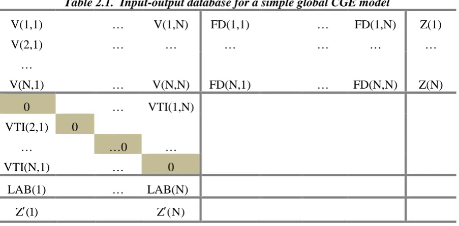
Global CGE models are built around input-output databases. Table 2.1 is illustrative for a simple N-region global CGE model in which labour is the only primary factor input and tariffs on intermediate flows are the only wedges between factory door prices and purchasers’ prices.
In Table 2.1, V(r,d) is a C by C matrix where C is the number of commodities or industries. The h,k component of V(r,d) is the pre-tariff value of commodity h produced in region r used in industry k in region d. VTI(r,d) is the C by C matrix of tariff collections associated with V(r,d). FD(r,d) is a C by 1 vector in which the h component is the value of commodity h from country r used in final demand in country d. Because we assume no trade in the final Widget commodity, we do not need to allow for tariffs on final goods to illustrate how the GSC and CGE models can be integrated. Thus, for simplicity we assume no tariffs on any
final good. LAB(r) is a 1 by C vector in which the k component is the value of labour input to industry k in region r. Z(r) is the C by 1 vector of sales values of commodities produced in region r. Its transpose,Z (r)′ , is the 1 by C vector of total costs incurred by industries in region r. A fundamental balance condition in CGE models is that the value of sales of each commodity produced in each region is equal to costs in the producing industry. In Table 2.1, these costs are the value of labour plus intermediate goods including tariffs on intermediates.
One interpretation of CGE models is that they are a system of equations that drive the components of an input-output database. The variables in the CGE model that combine to determine the value of each input-output flow are quantities and factory prices. Quantities are determined in cost-minimizing and utility-maximizing problems. Purchasers’ prices reflect factory prices (costs) and tariffs. In this stylized example, we leave out sales taxes and transport costs. Factory prices are determined by wages and by technology (input
12
either exogenous or modelled via demographic variables. Total final demand in each region depends on incomes, which depend on wages.
In a typical global CGE model we can think of Widgets as a single commodity and industry in each region. The Widget row of the input-output data for region r shows Widget sales to the Widget industry and other parts of region r’s economy as well as Widget sales to export. The Widget column for region r shows inputs to Widget production in region r and associated tariffs.
Given the specification of the global Widget sector in subsection 2.1, what we would see in the Widget row for source region r in the input-output data in Table 2.1 is zero entries except (possibly) in the Widget-Widget or WW position of the V(r,d) matrices and the W position of the FD(r,r) vector. This is because Widgets are traded only as intermediate inputs to Widget industries. What we would see in the Widget column for destination region d is zero entries except for the Widget entry in LAB(d) and (possibly) the WW entries in V(r,d) for all r and VIT(r,d) for all r ≠ d.
What we would not see in the input-output data is the underlying nature of the Widget flows. With the GSC Widget specification in subsection 2.1, the intermediate inputs to region d’s Widget industry and Widget exports from region d would be aggregations of commodities in WCI. Region d’s domestic Widget sales outside the Widget sector would consist entirely of the final good. But these features are not revealed by the input-output data: we simply see undifferentiated flows of Widgets.
In essence, our approach to integrating GSC and CGE models is to devise a method for driving the undifferentiated Widget flows and primary factor inputs to the Widget industry in each region in the CGE model in a way that takes account of the underlying changes in activities in the GSC model. To do this, we must work out how output, input and price variables for the undifferentiated Widget commodity/industry in each region in the CGE model should react to changes in output, input and price variables for the underlying Widget activities in the GSC model.
2.3. Integrating GSC and CGE: sharing roles between the two models in an integrated system
Looked at through a CGE lens, the channels through which a GSC Widget sector affects the broader economy in each region include:
(a) the price of the final Widget good;
(b) demands for domestic and imported inputs per unit of output in the Widget sector; (c) demands for primary-factor inputs per unit of output in the Widget sector; and (d) average tariff rates in each region on imports of Widget goods.
If developments (e.g. productivity improvements) in the Widget sector of region d lead to lower prices for the final Widget good, then imposed on a CGE model this will produce a series of repercussions. These may include increased consumption of Widgets in region d, increased or reduced consumption of other goods depending on trade-offs between
13
Table 2.1. Input-output database for a simple global CGE model
V(1,1) … V(1,N) FD(1,1) … FD(1,N) Z(1)
V(2,1) … … … …
…
V(N,1) … V(N,N) FD(N,1) … FD(N,N) Z(N)
0 … VTI(1,N)
VTI(2,1) 0
… …0 …
VTI(N,1) … 0
LAB(1) … LAB(N)
Z (1)′ Z (N)′
Looked at through a GSC lens, the channels through which the broader multi-region economy affects the Widget sector in each region include:
(e) wage rates; and
(f) Widget demand by final users.
To integrate a CGE and a GSC model we impose on the CGE model outcomes from the GSC model for (a) to (d) and impose on the GSC model outcomes from the CGE model for (e) and (f). In this way, we ensure that Widget variables in the CGE model are driven by the GSC model and economy-wide variables in the GSC model are driven by the CGE model.
In the case of the GSC and CGE models described in sections 2.1 and 2.2, we say that they are fully integrated if and only if
(i) wage rates and final demand for Widgets used in determining the GSC solution are the same as those determined in the CGE model;
(ii) the power of the tariff, and the value of the flow and related tariff collection for the single Widget commodity applying to any pair of regions r and d in the CGE model is the value of these variables determined in the GSC model as appropriate aggregations over Widget commodities of powers, values and tariff collections;
(iii) the technology (intermediate and primary-factor input per unit of output) in each region’s Widget industry in the CGE model is the same as that for the Widget sector in the GSC model derived by appropriate aggregation over the four Widget activities; (iv) the price of region r’s single Widget good in the CGE model is the price of r’s final
Widget good determined in the GSC model; and
(v) employment in each region’s Widget industry in the CGE model is the same as that for the Widget sector in the GSC model derived by adding over Widget activities.
Through conditions (i) to (v) we are saying that two models are fulling integrated if there are no inconsistencies between them in their solutions for variables of relevance to welfare and resource allocation.
14
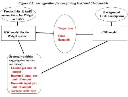
Figure 2.1. An algorithm for integrating GSC and CGE models
demands for Widgets, the GSC model produces results for Widget activities. From these, movements for each region in inputs per unit of output and average tariff rates at the
aggregated sectoral level for Widgets can be calculated. As shown in the figure, these can be passed to the CGE model. The CGE model can also receive shocks to the myriad of
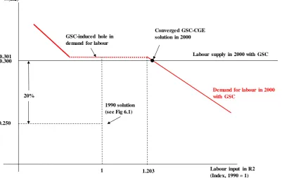
technology, tariff and other exogenous CGE variables outside the Widget sector. The CGE model then produces results for wage rates and final demands for Widgets in each region. Starting with a CGE solution incorporating initial guesses for Widget sectoral variables or with a GSC solution incorporating initial guesses for wage rates and final demands for Widgets, we can follow the arrows around Figure 2.1 looking for a converged solution. A converged solution occurs when wage rates and final demands being passed to the GSC model are unchanged between successive iterations or equivalently when the Widget sectoral variables being passed to the CGE model are unchanged between successive iterations.
As demonstrated in the Appendix, full integration between the GSC Widget model and a CGE model is achieved by computing fully converged solutions. By computing such solutions we can reveal (1) the economy-wide (CGE) effects of shocks to productivity and tariffs applying to GSC activities and (2) the intra-widget (GSC) effects of shocks to exogenous CGE variables such as changes in productivity in sectors apart from Widgets.
Will the algorithm converge? We were confident that this algorithm or a variant of it (e.g. partial adjustment between steps) would work because the GSC sector is usually quite a small fraction of the total economy. Consequently, we expected wages and final demands
determined in the broader economy to be relatively insensitive to developments in the GSC sector. However, as explained in section 6, in a stylized example there was sufficient
Background CGE assumptions
GSC model for the Widget sector
CGE model
Wage rates
Final demands
Sectoral variables (aggregated across activities):
Labour per unit of output
Imported input per unit of output Domestic input per
unit of output Average tariff rate
Productivity & tariff assumptions for Widget
15
sensitivity of wages to GSC developments that convergence could not be achieved without an important modification to the standard CGE model.
3. A GSC sector in a CGE database: an illustrative numerical example
In this section, we provide a numerical example showing how a GSC sector is represented in a world input-output database of the type used in CGE modelling. We assume that there are two regions, R1 and R2, which we will think of as the U.S. and Asia, and two industries, Ind1 and Ind2. Ind1 is a potential GSC industry while Ind2 is the rest of the economy consisting mainly of services but also including tradable goods such as agriculture and mining.
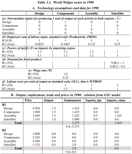
For Ind1 we adopt a special case of the Widget industry in the GSC model described in subsection 2.1. Within this Widget industry, there are four activities: Design; Components; Assembly; and SalesDist. Data for these four activities are given in Table 3.1, part A. For concreteness, we will think of these data as referring to 1990.
As shown in the top panel of Table 3.1A: production of a unit of Components requires 1 unit of Design; production of a unit of Assembly requires 1 unit of Components; and production of a unit of SalesDist requires 1 unit of Assembly. In terms of the model in subsection 2.1, this defines A on the LHS of (2.5). Panel (b) in Table 3.1A gives the values for labour productivity in each Widget activity at standard scale [PROD in (2.6)]. As explained in subsection 2.1, we assume that labour productivity in activity j in region r is 5 per cent greater than PROD if r undertakes all of the output of j required for both regions (see the definition of SCALE). Panel (c) gives the powers of the tariffs [T in (2.8)] and panel (e) gives wage rates [W in (2.6)]. SalesDist is the non-traded final Widget commodity. Quantities of this commodity [Y in (2.4)] used in each region are given in panel (d).
Panel (f) in Table 3.1A shows wage rates divided by PROD, that is labour costs per unit of output at standard scale for each Widget activity in the two regions. Even though wage rates are much lower in R2 than in R1, wage costs per unit of output in all traded Widget activities are higher in R2 than in R1. This reflects the very low productivity levels assumed for R2 in panel (b) relative to those for R1.
Part B of Table 3.1 shows the GSC Widget solution generated under the assumptions in Part A. In view of the high labour costs per unit of output applying to Design, Components and Assembly in R2, it is not surprising that R1 is dominant in world production of these three traded Widget commodities. The only non-zero Widget activity in R2 is production of the non-traded commodity SalesDist. Despite a tariff of 20 per cent, R2 satisfies all of its
requirement for Assembly by importing from R1. Imported Assembly goes to R2’s SalesDist activity. Because R2 does not produce either Components or Assembly, it does not import either Design or Components.
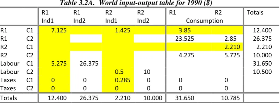
The shaded parts of Table 3.2A depict the Widget industry of Tables 3.1A&B in a world input-output database of the form used in CGE modelling. In this database, Widgets is industry 1 (Ind1). It is represented as producing a single composite commodity (C1). The underlying details of Design, Components, Assembly and SalesDist are supressed.
Exports of Widgets (C1) from R1 to R2 are shown in Table 3.2A with a cif value of 1.425. This consists of 0.5 units of Assembly priced at 2.850 per unit (see Table 3.1B).
16
Table 3.1. World Widget sector in 1990
A. Technology assumptions and data for 1990
Design Components Assembly SalesDist
(a) Intermediate inputs for producing 1 unit of output of each activity in both regions (A)
Design 0 1 0 0
Components 0 0 1 0
Assembly 0 0 0 1
SalesDist 0 0 0 0
(b) Output per unit of labour input, standard scale (Productivity, PROD)
R1(US) 1 1 1 1
R2 (Asia) 0.0833 0.1667 0.125 0.25
(c) Powers of tariffs (T) on imports by importing region
R1 (US) 1.1 1.2 1.2 1
R2 (Asia) 1.1 1.2 1.2 1
(d) Demand for final product:
R1 (US) Y(R1) = 1
R2 (Asia) Y(R2) = 0.5
(e) Wage rate (W)
R1 (US) 1.0
R2 (Asia) 0.25
(f) Labour costs per unit of output at standard scale (SLC), that is W/PROD
R1 (US) 1 1 1 1
R2 (Asia) 3 1.5 2 1
B. Output, employment, trade and prices in 1990: solution from GSC model
Price Output Employment Exports, qty Exports, value R1
Design 0.950 1.5 1.425 0.0 0.0
Components 1.900 1.5 1.425 0.0 0.0
Assembly 2.850 1.5 1.425 0.5 1.425
SalesDist 3.850 1.0 1.000 0.0 0.0
Total 5.275 1.425
VA=5.275
R2
Design 3.000 0.0 0.0 0.0 0.0
Components 2.545 0.0 0.0 0.0 0.0
Assembly 4.280 0.0 0.0 0.0 0.0
SalesDist 4.420 0.5 2.0 0.0 0.0
Total 2.0 0.0
VA=0.5
The values in Table 3.2A of labour input to Ind1 in the two regions (5.275 and 0.5) are simply the value added (VA) numbers in Table 3.1B. These numbers are the wage rates in the two regions (1.0 and 0.25, Table 3.1A) multiplied by the Widget employment levels (5.275 and 2.0, Table 3.1B).
17
Table 3.2A. World input-output table for 1990 ($)
R1 R1 R2 R2 R1 R2 Totals
Ind1 Ind2 Ind1 Ind2 Consumption
R1 C1 7.125 1.425 3.85 12.400
R1 C2 23.525 2.85 26.375
R2 C1 2.210 2.210
R2 C2 4.275 5.725 10.000
Labour C1 5.275 26.375 31.650
Labour C2 0.5 10 10.500
Taxes C1 0 0 0.285 0 0 0
Taxes C2 0 0 0 0 0 0
Totals 12.400 26.375 2.210 10.000 31.650 10.785
The numbers in the shaded rows and columns are for flows of commodity 1 (C1) and inputs to industry 1 (Ind1) that produces C1. These numbers are obtained from the Widget data in Table 3.1. The numbers for C2 and Ind2 were set so that the Widget Industry (manufacturing) contributes approximately 17 per cent of GDP in region 1 (R1) and 5 per cent of GDP in region 2 (R2).
Table 3.2B. World input-output table for 1990 ($) modified for use in CGE model
R1 R1 R2 R2 R1 R2 Totals
Ind1 Ind2 Ind1 Ind2 Consumption
R1 C1 7.125 1.425 3.85 12.400
R1 C2 23.525 2.85 26.375
R2 C1 0.01 0.01 2.200 2.220
R2 C2 4.265 5.735 10.000
Labour C1 5.265 26.375 31.640
Labour C2 0.5 10 10.500
Taxes C1 0 0 0.285 0 0 0
Taxes C2 0 0 0 0 0 0
Totals 12.400 26.375 2.220 10.000 31.640 10.785
We can calculate the value of Widget consumption shown in Table 3.2A for each region as the value of output plus imports less exports less intermediate use. For R1 this gives consumption of Widgets at 3.85 (= 12.4 +0 – 1.425 – 7.125). For R2, consumption of
Widgets is 2.21 (= 2.21 +1.425 – 0 – 1.425). These consumption values can be checked from Table 3.1. They are the consumption (or output) quantities of SalesDist (1 and 0.5, Table 3.1A) times the prices of SalesDist (3.850 and 4.420, Table 3.1B).
For simplicity we assume that Ind2 in each region uses only labour as an input and sells only to final demand. We also assume there are no tariffs on trade in Ind2’s product (C2). In both regions, Ind2 is much larger than Ind1. As shown in Table 3.2A, Ind2 accounts for 83.33 per cent of employment in R1 (26.375 out of 31.650) and 95.24 per cent in R2 (10 out of 10.5).
We assume that trade in 1990 is balanced. Reflecting its specialization in Widgets, R1 has a Widget trade surplus of 1.425 while R2 has a surplus of 1.425 in C2 trade ( = 4.275 – 2.85)
18
reducing labour input to Ind1 in R1 by 0.01 and reducing consumption of C1 in R2 by 0.01, to arrive at Table 3.2B. In rebalancing, we preserve the original trade balances, zero for each region.
4. Baseline CGE forecast
Imagine that we are standing in 1990 trying to project forward to 2000. We have the input-output database set out in Table 3.2B and decide to build a standard CGE model calibrated to this database. In the model, we assume that: production functions for the two industries in each of the two regions are Leontief in intermediate inputs of C1 and C2 and the single primary factor labour; household preferences are Cobb-Douglas between C1 and C2; and Armington elasticities set at 3.8 determine substitution by industries and households between imported and domestic varieties of the same commodity. In modelling each labour and intermediate input, we allow for technical change by introducing an exogenous variable that affects the use of the input per unit of output.
Shocks
In applying this CGE model to the task of projecting from 1990 to 2000, we introduce three ideas. First, R2 (Asia) is rapidly catching up to R1 (U.S.) in terms of productivity and wages. Second, productivity growth is rapid in Ind1 (think manufacturing) relative to Ind2
(dominated by services). Third, tariffs are being dismantled. Looking at these ideas through CGE eyes, we project from 1990 to 2000 by applying the following shocks:
(1) labour-saving technical progress in Ind1, R1 = 15% (2) labour-saving technical progress in Ind2, R1 = 0% (3) labour-saving technical progress in Ind1, R2 = 27.75% (4) labour-saving technical progress in Ind2, R2 = 15%
(5) reduction in the power of the tariff on R2’s imports of C1 = 12.5%
Shocks (1) and (2) give R1 a background rate of labour-saving technical change of 0% with 15% extra for Ind1. Shocks (3) and (4) give R2 a background rate of labour-saving technical change of 15% with 15% extra for Ind1. The 15% extra means that instead of falling from 1 to 0.85, the index of labour requirements per unit of output in R2’s Widget industry falls from 1 to 0.7225 ( = 0.85*0.85). Shock (5) introduces a reduction in the rate of the tariff imposed by R2 on imports of C1 from 20% to 5% [-12.5= 100*(1.05/1.20 - 1)].
In this section, and later in sections 7 and 8, we assume no change in both regions in
employment measured in people. In generating standard CGE forecasts, we also assume no growth in aggregate labour input (row 22, Table 4.1), implying that labour input is adequately measured by employment (number of people employed). In sections 7 and 8, describing results from the integrated GSC-CGE model, we allow for changes in labour input associated with movement of surplus but employed labour from Ind2 to Ind1 in R2.
We could add other shocks to (1) - (5).2 For example, we could include shocks to the number of people employed in each region reflecting demographic developments and to the trade balance reflecting capital flows. These variables are exogenous in our projections. Correspondingly, real wage rates and real exchange rates are endogenous. However, including shocks to employment and the trade balance is unnecessary for our current illustrative purposes.
2 We did in fact include a sixth shock to deal with a minor problem caused by inclusion in the 1990 database of the artificial
19 Results
Table 4.1 shows the projections for R1 and R2 derived by applying shocks (1) to (5) to our stylized CGE model. With no capital in this simple model and with no growth in labour input, the projected increases in real GDP (row 1) can be explained purely from our
technology assumptions and items in the input-output data in Table 3.2B. R1 is projected to have labour-saving technical progress of 15 per cent [shock (1)] in 16.67 per cent of its economy (Ind1’s share of R1’s labour input) giving it a GDP increase of about 2.6 per cent, close to the number shown in Table 4.1 (2.72, row 1, col 1). R2 is projected to have labour-saving technical progress of 27.75 per cent [shock (3)] in about 4.76 per cent (Ind1) of its economy and 15 per cent [shock (4)] in about 95.24 per cent (Ind2) of its economy. For a given level of output this technical progress frees up about 15.6 per cent of the labour force. Re-employing this labour enables R2 to increase its GDP by about 18.5 per cent [=
100*0.156/(1-0.156)], which is close to the result in Table 4.1 (18.76, row 1, col 2).
Rapid technical progress in R2 relative to R1 gives workers in R2 a wage increase of 13.82 per cent relative to workers in R1 (row 3 in Table 4.1).3 In real terms the wage increase in R2 is nearly 20 percentage points greater than that in R1 (row 4). The wage differential is accentuated in real terms by the improvement in R2’s terms of trade (discussed below) and by the cut in its tariffs on its imports of C1 [shock (5)].4
Reflecting the 1990 situation of balanced trade and the assumption of no-change in the trade balance, real consumption (row 2, Table 4.1) in the two regions increases broadly in line with GDP. Small GDP-consumption discrepancies arise from terms-of-trade movements: a
slightly smaller percentage increase in consumption than in GDP in R1 (2.41 compared with 2.72) and a slightly larger increase in R2 (19.76 compared with 18.76). R2 benefits from a terms-of-trade improvement (row 15) which increases the amount of consumption that it can undertake per unit of output (or GDP). The reverse is true for R1. R2 experiences a terms-of-trade improvement because it is a net exporter of C2 and it imports C1: prices for C1 fall relative to those for C2 (rows 5 to 8) reflecting extra technical progress in the production of C1 relative to C2.
With balanced trade and strong growth in R2 relative to R1, R2’s trade falls as a share of GDP [real export growth of 12.84 per cent (row 13) compared with GDP growth of 18.76 per cent]. The explanation is that the export market for R2 (namely R1) is shrinking relative to the size of R2’s domestic market. The opposite is true for R1.
Rows 16 to 21 show developments at the industry/commodity level. In both regions, labour input in industry 1 declines relative to that in industry 2 (rows 16 and 17). For R1, the
decline is about 1.80 per cent (= 1.51+0.30) and for R2 it is about 4.5 per cent (= 4.29+0.21). These declines are brought about by rapid technical progress in Ind1 relative to Ind2. They can be accommodated by small switches between industries in labour input. In R1, labour input in Ind1, which accounts for 16.6 per cent of R1’s total labour input in 1990 (Table 3.2B), falls by 1.51 per cent. With no change in aggregate labour input this implies a reallocation between 1990 and 2000 of 0.25 per cent of R1’s workforce from Ind1 to Ind2 (= 1.51*0.166). The workforce-switch percentage is even smaller for R2, 0.20 per cent.
3 The wage rate in R1 is the numeraire. Consequently, it is shown in Table 4.1 with zero change.
4 A cut in tariffs, as with a cut in any indirect tax, allows a given level of employment to be maintained with a
20
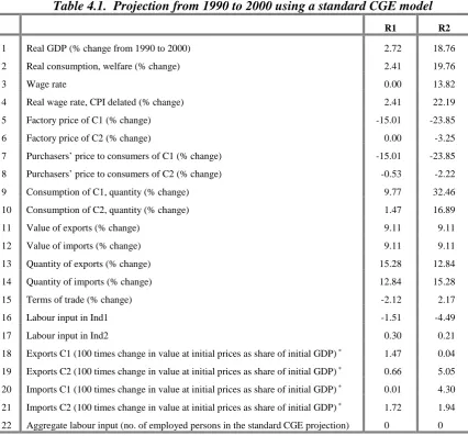
Table 4.1. Projection from 1990 to 2000 using a standard CGE model
R1 R2
1 Real GDP (% change from 1990 to 2000) 2.72 18.76 2 Real consumption, welfare (% change) 2.41 19.76
3 Wage rate 0.00 13.82
4 Real wage rate, CPI delated (% change) 2.41 22.19 5 Factory price of C1 (% change) -15.01 -23.85 6 Factory price of C2 (% change) 0.00 -3.25 7 Purchasers’ price to consumers of C1 (% change) -15.01 -23.85 8 Purchasers’ price to consumers of C2 (% change) -0.53 -2.22 9 Consumption of C1, quantity (% change) 9.77 32.46 10 Consumption of C2, quantity (% change) 1.47 16.89 11 Value of exports (% change) 9.11 9.11 12 Value of imports (% change) 9.11 9.11 13 Quantity of exports (% change) 15.28 12.84 14 Quantity of imports (% change) 12.84 15.28 15 Terms of trade (% change) -2.12 2.17
16 Labour input in Ind1 -1.51 -4.49
17 Labour input in Ind2 0.30 0.21
18 Exports C1 (100 times change in value at initial prices as share of initial GDP) * 1.47 0.04
19 Exports C2 (100 times change in value at initial prices as share of initial GDP) * 0.66 5.05
20 Imports C1 (100 times change in value at initial prices as share of initial GDP) * 0.01 4.30
21 Imports C2 (100 times change in value at initial prices as share of initial GDP) * 1.72 1.94
22 Aggregate labour input (no. of employed persons in the standard CGE projection) 0 0
* 100*(Quantity in final year times price in initial year – Value in initial year)/GDP in initial year
Rows 18 to 21 show changes in the commodity composition of each region’s trade. In these rows, it is convenient to report changes in volume flows as percentage-point changes in shares of initial GDP. For example, the entry in the R1 column of row 18 means that between 1990 and 2000 R1’s exports of C1 valued at 1990 prices increased as a share of initial GDP by 1.47 percentage points, that is, from 4.5038 per cent of GDP in the 1990 database in Table 3.2B to 5.9693 per cent. In this case, the volume increase is finite and interpretable, 32.54 per cent [=100*(5.9693/4.5038-1)]. However, as we will see in section 8, our integrated GSC-CGE model can generate substantial trade flows for 2000 from an arbitrarily small starting point in 1990, making percentage change results uninformative. By reporting percentage-point share changes in GDP, we not only avoid this problem but we also highlight changes in the commodity structure of trade.
Viewed this way, the trade projections in Table 4.1 can be described as “business as usual”. In 1990, R2 specialized in the export of C2 (4.265 out of total exports 4.275, see Table 3.2B). This specialization continues in 2000 with the expansion of R2’s exports accounted for
21
comparative advantage in the production of C1 is preserved. Given the relative weakness of R2 in the production of C1, R2’s consumers draw strongly on R1 to satisfy their rapidly growing demand for C1. This explains the growth in R1’s exports of C1 (row 18) relative to its exports of C2 (row 19).
The import results in rows 20 and 21 of Table 4.1 follow in a mechanical way from the export results. Consequently, no further explanation is required.
5. World Widget industry in 2000: technology and tariff assumptions, and GSC solution
Now imagine that we are specialists on the Widget industry, wishing to project the industry’s prospects from 1990 to 2000 using the GSC model described earlier. Our views on
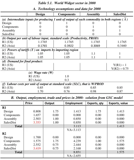
exogenous variables for the Widget industry in 2000 are shown in Table 5.1 part A and our assumptions concerning movements in these variables from their 1990 values can be deduced by comparing Table 5.1A with Table 3.1A.
As in 1990, we assume for 2000 that: one unit of Design is required per unit of Components; one unit of Components is required per unit of Assembly; and one unit of Assembly is required per unit of SalesDist.
Consistent with the assumptions we made as CGE modellers, we assume as GSC modellers that between 1990 and 2000 there will be labour-saving technical change of 15 per cent in R1’s Widget industry, and that this applies to the four Widget activities. For 1990 output per unit of labour in the four activities in R1 at standard scale was one (Table 3.1A). Thus, as shown in panel (b) of Table 5.1A, R1’s output per unit of labour at standard scale in the four activities in 2000 is assumed to be 1.1765 [= 1/(1-0.15)].
As CGE modellers in section 4 we assumed labour-saving technical progress between 1990 and 2000 in R2’s Widget industry of 27.75 per cent, made up of 15 per cent background labour-saving technical progress applying generally in R2 plus an extra 15 per cent in Ind1. In 1990 the only Widget activity in R2 was SalesDist (Table 3.1B). Now as GSC modellers we assume that the 27.75 per cent labour-saving technical progress applies in R2 to this activity. This assumption is reflected in panels (b) of Tables 3.1A and 5.1A which show an increase in PROD for SalesDist in R2 from 0.25 in 1990 to 0.3460 in 2000.5 In each of the other three Widget activities we assume that PROD in R2 more than doubles from its very low levels in 1990. Despite this, as can be seen from Table 5.1A panel (b), we assume that R2’s productivity levels in traded Widget activities in 2000 remain well below those in R1.
On tariffs, we note the trend towards free trade. As can be seen from panels (c) in Tables 5.1A and 3.1A, we assume that this trend applies to the Widget industry, and that tariffs on Design will fall from 10 per cent in 1990 in both regions to 5 per cent in 2000. For
Components we assume a fall from 20 per cent to 5 per cent and for Assembly a fall from 20 per cent to 10 per cent.
In our role as Widget specialists wishing to apply the GSC model, we need to make
assumptions about economy-wide wage rates and final demands for Widgets (demands for the product SalesDist). These assumptions must be guided by movements in productivity and income outside the Widget industry. Comparing panels (d) and (e) in Tables 5.1A with the corresponding panels in 3.1A shows our wage and demand assumptions: 20 per cent wage and 50 per cent demand growth in R2, and zero growth in these variables in R1. This is consistent with rapid catch-up by R2.
5 Labour-saving technical progress of 27.75 per cent means that a given level of output can be produced with 27.75 per cent
22
Table 5.1. World Widget sector in 2000
A. Technology assumptions and data for 2000
Design Components Assembly SalesDist
(a) Intermediate inputs for producing 1 unit of output of each commodity in both regions (A)
Design 0 1 0 0
Components 0 0 1 0
Assembly 0 0 0 1
SalesDist 0 0 0 0
(b) Output per unit of labour input, standard scale (Productivity, PROD)
R1 (US) 1.1765 1.1765 1.1765 1.1765
R2 (Asia) 0.1765 0.3922 0.3069 0.3460
(c) Powers of tariffs (T ) on imports by importing region
R1 (US) 1.05 1.05 1.1 1
R2 (Asia) 1.05 1.05 1.1 1
(d) Demand for final product:
R1 (US) Y(R1) = 1
R2 (Asia) Y(R2) = 0.75
(e) Wage rate (W)
R1 (US) 1.0
R2 (Asia) 0.3
(f) Labour costs per unit of output at standard scale (SLC), that is W/PROD
R1 (US) 0.85 0.85 0.85 0.85
R2 (Asia) 1.70 0.76 0.98 0.87
B. Output, employment, trade and prices in 2000: solution from GSC model
Price Output Employment Exports, qty Exports, value R1
Design 0.808 1.75 1.413 1.75 1.413
Components 1.657 0.00 0.000 0.00 0.000
Assembly 2.503 1.00 0.850 0.00 0.000
SalesDist 3.353 1.00 0.850 0.00 0.000
Total 3.113 1.413
VA=3.113
R2
Design 1.700 0.00 0.000 0.00 0.000
Components 1.575 1.75 4.239 1.00 1.575
Assembly 2.552 0.75 2.444 0.00 0.000
SalesDist 3.419 0.75 2.168 0.00 0.000
Total 8.851 1.575
VA=2.655
Given the assumptions in Table 5.1A, our GSC model produces the solution shown in Table 5.1B. Comparing this 2000 solution with the 1990 solution (Table 3.1B), we see that
production of Components has switched entirely from R1 to R2. Although R2’s productivity in Components in 2000 is low relative to that in R1, R2’s wage rate remains sufficiently low relative to that in R1 to give R2 a competitive edge in Component production. As can be seen from panel (f) in Table 5.1A, labour cost at standard scale per unit of output in
Components in R2 in 2000 is less than that in R1 (0.76 compared with 0.85). For Assembly production, R2’s labor cost per unit of output remains above that in R1 in 2000 (0.98
23
needs. R1 continues to produce Assembly but no longer exports. Why shouldn’t R1 continue to produce all of the Assembly required by both regions?
Given that Components are entirely produced in R2, splitting Assembly production not only saves trade costs (tariff payments) on Assembly but also on Components. It turns out that the saving of trade costs more than offsets the now relatively small reduction in world Assembly costs that would follow from leaving R1 as the sole Assembler.
With the complete switch of world Components productions and the partial switch of Assembly production from R1 to R2, together with rapid productivity growth, Widget employment in R1 declines sharply, from 5.275 in 1990 to 3.113 in 2000. By contrast, Widget employment in R2 increases sharply, from 2 in 1990 to 8.851 in 2000. R1’s 1990 trade surplus in Widgets of 1.425 (Table 3.1B) turns into a 2000 trade deficit of 0.162 (= 1.575-1.413, Table 5.1B).
6. Iterating to impose the GSC solution on the CGE model: a non-converging case
In the GSC Widget solution for 2000 we assumed wage and Widget demand increases
between 1990 and 2000 in R1 of zero and in R2 of 20% and 50%. If Widget productivity and tariff movements for 1990 to 2000 were as assumed in our GSC model, what would a CGE model tell us about wage rates and Widget demands?
In section 2 (see Figure 2.1) we described an algorithm that aims to ensure consistency: (a) between wage and Widget demand assumptions in GSC solutions and outcomes for these variables in CGE solutions; and (b) between tariff and Widget technology assumptions in CGE solutions and outcomes for these variables in GSC solutions. Achievement of these consistencies is what we call integration of the models.
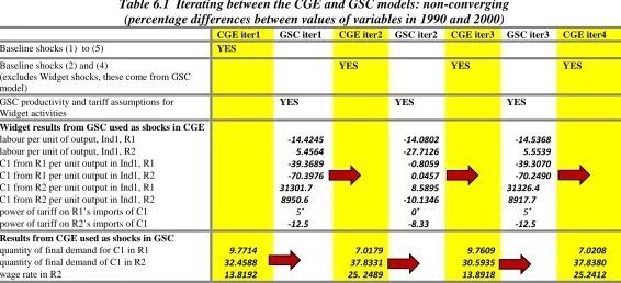
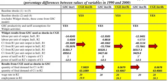
Table 6.1 shows our first attempt to implement the consistency algorithm. We started with CGE iter1. This is the baseline CGE solution described in section 4. In incorporates the shocks listed in section 4 together with the assumption of no change in labour input in either region. As shown in the CGE iter1 column of Table 6.1, this solution implies a wage increase in R2 of 13.8192 per cent (zero in R1 by the numeraire assumption) and Widget demand increases in R1 and R2 of 9.7714 and 32.4588 per cent. These results can also be seen (with less decimal places) in rows 3 and 9 of Table 4.1.
In GSC iter1 we solve the GSC model with the Widget assumptions given in Table 5.1A except that the wage (W) and final demand assumptions (Y) are replaced by results from CGE iter1.6 This replacement is indicated by the arrow from the CGE iter1 column in Table 6.1 to the GSC iter1 column. After the GSC model is solved with these new W and Y values, selected results are passed to the CGE model.
The block of selected GSC results from GSC iter1 that are passed to the CGE model are indicated by the arrow from the GSC iter1 column to the CGE iter2 column. These GSC results show percentage changes between 1990 and 2000 in labour and intermediate inputs per unit of output in each region’s Widget industry and also average powers of tariffs. Inputs, output and powers of tariffs are derived for each region’s Widget industry as a whole by aggregating results for Widget activities in the GSC model. The aggregation formulas are in the Appendix.
6 Instead of W(R2) = 0.3 as in Table 5.1A, in GSC iter1 we use W(R2) = 0.2845 (i.e. the 1990 value, 0.25, times 1.138192).
24
Table 6.1 Iterating between the CGE and GSC models: non-converging (percentage differences between values of variables in 1990 and 2000)
CGE iter1 GSC iter1 CGE iter2 GSC iter2 CGE iter3 GSC iter3 CGE iter4
Baseline shocks (1) to (5) YES
Baseline shocks (2) and (4)
(excludes Widget shocks, these come from GSC model)
YES YES YES
GSC productivity and tariff assumptions for Widget activities
YES YES YES
Widget results from GSC used as shocks in CGE
labour per unit of output, Ind1, R1 -14.4245 -14.0802 -14.5368 labour per unit of output, Ind1, R2 5.4564 -27.7126 5.5539 C1 from R1 per unit output in Ind1, R1 -39.3689 -0.8059 -39.3070 C1 from R1 per unit output in Ind1, R2 -70.3976 0.0457 -70.2490 C1 from R2 per unit output in Ind1, R1 31301.7 8.5895 31326.4 C1 from R2 per unit output in Ind1, R2 8950.6 -10.1346 8917.7 power of tariff on R1’s imports of C1 5* 0* 5* power of tariff on R2’s imports of C1 -12.5 -8.33 -12.5
Results from CGE used as shocks in GSC
quantity of final demand for C1 in R1 9.7714 7.0179 9.7609 7.0208 quantity of final demand of C1 in R2 32.4588 37.8331 30.5935 37.8380
wage rate in R2 13.8192 25.2489 13.8918 25.2412
* As shown in Table 3.2B, in 1990 R1 collected zero tariff revenue on negligible but non-zero imports of C1. These data imply (artificially) that the power of the tariff on R1’s imports of C1 was