Scholarship@Western
Scholarship@Western
Electronic Thesis and Dissertation Repository
9-6-2011 12:00 AM
The Analysis of Extreme Synoptic Winds
The Analysis of Extreme Synoptic Winds
David A. Gatey
The University of Western Ontario
Supervisor Dr. Craig Miller
The University of Western Ontario
Graduate Program in Civil and Environmental Engineering
A thesis submitted in partial fulfillment of the requirements for the degree in Doctor of Philosophy
© David A. Gatey 2011
Follow this and additional works at: https://ir.lib.uwo.ca/etd
Part of the Civil and Environmental Engineering Commons, and the Meteorology Commons
Recommended Citation Recommended Citation
Gatey, David A., "The Analysis of Extreme Synoptic Winds" (2011). Electronic Thesis and Dissertation Repository. 268.
https://ir.lib.uwo.ca/etd/268
This Dissertation/Thesis is brought to you for free and open access by Scholarship@Western. It has been accepted for inclusion in Electronic Thesis and Dissertation Repository by an authorized administrator of
by
David Allan Gatey
Graduate Program in Civil and Environmental Engineering
A thesis submitted in partial fulfillment
of the requirements for the degree of
Doctor of Philosophy
The School of Graduate and Postdoctoral Studies
The University of Western Ontario
London, Ontario, Canada
c
CERTIFICATE OF EXAMINATION
Supervisor:
. . . . Dr. C.A. Miller
Supervisory Committee:
. . . . Dr. H. Hangan
. . . . Dr. E. Savory
Examiners:
. . . . Dr. W.J. Braun
. . . . Dr. H.P. Hong
. . . . Dr. M. Kasperski
. . . . Dr. G.A. Kopp
The thesis by
David Allan Gatey
entitled:
The Analysis of Extreme Synoptic Winds
is accepted in partial fulfillment of the requirements for the degree of
Doctor of Philosophy . . . .
Date
. . . . Chair of the Thesis Examination Board
Time histories of wind speed and direction from 394 surface observation stations were ob-tained to calculate synoptic 50-year return period wind speeds for 11 countries in Europe. Preliminary investigation indicated wind speed differences along national borders were suc-cessfully reduced by application of a simple consistent methodology to wind speed data. This study considers the ideal methodology for calculating synoptic 50-year return period wind speeds.
Wind speed data requires standardisation through quality control measures, exposure cor-rection and adjustment for disjunct sampling. A quality control algorithm was successfully applied to identify shifts of monthly mean wind speeds and data conversion issues. Three exposure correction models were evaluated and two-layer models were found to perform better than internal boundary layer models. The differences arise as a result of how the models adapt to an upstream change of roughness. Furthermore, an empirical model was formed to correct observations at stations which were not recording measurements hourly.
Extreme value analyses were carried out using a robust estimator to fit the extreme value distribution type I to storm and yearly maxima. The latter was found to provide more con-sistent results. Comparison of the resulting 50-year return period wind speeds to existing literature found that several regions were in good agreement, while other regions exhib-ited similar spatial variation but greater magnitudes. The differences in magnitude were partially related to exposure correction methods, thus lending support to the importance of a single consistent methodology. Directional factors were calculated and subsequently grouped into six regions exhibiting similar directional characteristics.
Background wind fields were calculated from mean sea-level pressure data using the geostrophic approximation and consideration of other improved approximations, however, variations in
riod wind field calculated from upper-level wind fields was significantly lower than surface wind speed estimates due to spatial and temporal smoothing. Finally, assimilation of the 50-year return period wind speeds from surface observations and the background wind field was explored using the Bratseth scheme for statistical interpolation. The Bratseth scheme provided an overall 50-year return period wind speed map.
Keywords: 50-year return period wind speeds, homogenising wind data, exposure
correc-tion, boundary layer, extreme value analysis, outliers, Bratseth, synoptic winds, European wind map
Work on a thesis quite often finishes as it starts, with many long hours and sleepless nights spent in the office. I could not have completed this thesis without the support of the tech-nical and support staffof the Boundary Layer Wind Tunnel Laboratory, my friends and, of course, family. Special thanks needs to be given to particular individuals who have been there on a daily basis since the beginning.
I thank my supervisor, Dr. Craig Miller, who took me on as a undergraduate research student over 7 years ago. He has always had an open door and the time to provide guidance and support throughout the course of this thesis. In addition, he provided me with the opportunity and means to speak at various international conferences and to get involved with, and occasionally distracted by, several interesting projects. I truly believe I am a more well-rounded and stronger researcher because of his guidance.
I would like to thank Tom Mara and Zach Taylor for the many interesting discussions and late evenings bouncing ideas offone another, or simply unwinding, over a good Islay.
To Laurie, thank you for your love and firm determination to ensure I finished this thesis on time. Your support, particularly over these final months, has been remarkable.
To both of my grandfathers, Cor Dorssers and Allan Gatey, who taught me the value of good, hard work and the importance of a strong education. I know that they would have been truly proud of what I have accomplished and, with both of their passings occurring in these final months, I dedicate this thesis to them.
Certificate of Examination ii
Abstract iii
Acknowlegements v
List of Figures ix
List of Tables xi
List of Appendices xii
1 Introduction 1
1.1 Overview . . . 1
1.2 Objectives . . . 3
2 Background 9 2.1 Preliminary Study . . . 9
2.2 Surface Data . . . 14
2.3 Station Selection . . . 16
3 Standardisation of Wind Speed Data 18 3.1 Quality Control Measures . . . 19
3.1.1 Background . . . 19
3.1.2 Global Quality Control Measures . . . 22
3.1.3 Localised Quality Control Measures . . . 26
3.1.4 Thunderstorm Identification . . . 29
3.2 Atmospheric Boundary Layer . . . 30
3.2.1 Background . . . 30
3.2.2 Gryning ABL Model . . . 33
3.3 Heterogeneous Exposure Correction . . . 35
3.3.1 Background . . . 35
3.3.2 Methodology . . . 39
3.3.3 Deaves and Harris IBL Model . . . 42
3.3.4 Hydra TL Model . . . 44
3.3.5 TL Model: Gryning ABL . . . 45
3.3.6 Beljaar’s Gustiness Model . . . 46
3.4.1 Background . . . 53
3.4.2 Methodology . . . 55
3.4.3 Results . . . 56
4 Statistical Methods for the Estimation of Extreme Winds 58 4.1 Classical Extreme Value Theory . . . 59
4.1.1 Generalised Extreme Value Distribution . . . 60
4.2 Estimators . . . 61
4.2.1 Maximum Likelihood Estimators . . . 63
4.2.2 Optimal Bias-Robust Estimators . . . 65
4.3 Outlier Identification . . . 66
4.4 Results . . . 68
4.4.1 Annual Maxima . . . 68
4.4.2 Storm Maxima . . . 70
4.4.3 Mapping . . . 75
4.4.4 Directionality . . . 86
5 Background Wind Field 91 5.1 Background . . . 92
5.2 ECMWF Re-analysis . . . 94
5.3 Wind Fields from Mean Sea Level Pressure Data . . . 94
5.3.1 Geostrophic Approximation . . . 96
5.3.2 Quasi-geostrophic Approximation . . . 97
5.3.3 Semi-geostrophic Approximation . . . 99
5.4 Wind Fields from Pressure-level Data . . . 103
5.5 Results . . . 105
6 Data Assimilation 112 6.1 Bratseth Scheme . . . 113
6.2 Methodology . . . 114
6.2.1 Bratseth Scheme . . . 116
6.3 Results . . . 116
7 Conclusions 119 7.1 Overview . . . 119
7.2 Conclusions . . . 121
7.2.1 Standardisation and Homogenisation of Wind Speed Data . . . 121
7.2.2 Extreme Value Analysis . . . 123
7.2.3 Background 50-year Return Period Wind Field . . . 125
7.2.4 Data Assimilation . . . 127
7.3 Future work . . . 128
References 129
B Statistical Methods 149
B.1 Generalised Extreme Value Distribution: Statistical Properties . . . 149
B.2 Influence Function . . . 151
B.2.1 Overview . . . 151
B.2.2 Derivation: Maximum Likelihood Estimators . . . 152
B.3 Optimal Bias-Robust Estimators . . . 154
B.3.1 Estimator . . . 154
B.3.2 Algorithm . . . 155
Curriculum Vitae 157
2.1 Regions of interest in Europe for the preliminary study . . . 10
2.2 Comparison of European 50-year return period wind speed maps . . . 12
2.3 Map of selected WMO stations . . . 17
3.1 Correlation of monthly mean wind speeds . . . 24
3.2 Quality control regions . . . 25
3.3 Global quality control measures . . . 25
3.4 Distribution of observations failing local quality control checks . . . 29
3.5 Fits of various wind profiles to the Leipzig wind profile . . . 34
3.6 CORINE LULC and sampling grid (meso- and local-scale) . . . 42
3.7 Directional exposure correction factors . . . 50
3.8 Comparison of correction factors for a smooth to rough transition . . . 51
3.9 Distribution of correction factors . . . 53
3.10 Disjunct sampling correction factors . . . 56
4.1 EVD type I fit to annual maxima with potential outlier . . . 69
4.2 Typical good-quality EVD type I fit to annual maxima . . . 71
4.3 Influence of storm threshold selection . . . 71
4.4 Influence of OBRE downweighting . . . 73
4.5 Typical good-quality EVD type I fit to storm maxima . . . 74
4.6 Distribution of 50-year return period wind speed differences . . . 75
4.7 Distribution of the A-D test statistic . . . 76
4.8 50-year return period wind speed zones (annual maxima) . . . 77
4.9 Comparison of European 50-year return period wind speed maps . . . 80
4.10 Elevation: USGS GTOPO30 . . . 81
4.11 Comparison of European 50-year return period wind speed maps . . . 84
4.12 Directional factors by nation . . . 90
5.1 MSLP field: Burns’ Day Storm (January, 1990) . . . 95
5.2 MSLP field: Anatol (December, 1999) . . . 95
5.3 Geostrophic wind field: Burns’ Day Storm . . . 98
5.4 Geostrophic wind field: Anatol . . . 98
5.5 Quasi-geostrophic wind field: Burns’ Day Storm . . . 100
5.6 Quasi-geostrophic wind field: Anatol . . . 100
5.7 Semi-geostrophic wind field: Burns’ Day Storm . . . 102
5.8 Semi-geostrophic wind field: Anatol . . . 102
5.9 Semi-geostrophic wind field (Smoothed MSLP): Burns’ Day Storm . . . 103
5.12 Wind field at 1000 m: Anatol . . . 106
5.13 50-year return period wind speeds adjusted for surface geopotential . . . . 107
5.14 50-year return period wind speeds unadjusted for surface geopotential . . . 107
5.15 Distribution of the location parameters . . . 109
5.16 Distribution of the scale parameters . . . 110
5.17 Comparison of mean background and surface EVD type I fits . . . 111
6.1 Example of the Bratseth Scheme . . . 115
6.2 50-year return period wind field - Bratseth scheme (D=125 km) . . . 117
6.3 50-year return period wind field - Bratseth scheme (D=250 km) . . . 117
1.1 Statistical methods used in wind engineering to analyse extreme winds . . . 6
2.1 Sources of 50-year return period wind speeds by country . . . 12
2.2 Classifications and associated criteria for station selection . . . 16
3.1 Summary of conversion errors by country . . . 26
3.2 Present weather and thunderstorm identifiers . . . 27
3.3 Localised quality control criteria . . . 28
3.4 LULC roughness assignments . . . 41
3.5 Comparison of the relative error from IBL and TL model correction factors 49 3.6 Disjunct sampling correction factor equations . . . 57
A.1 Listing of Selected Stations . . . 148
Appendix A Station Listing . . . 138 Appendix B Statistical Methods . . . 149
Introduction
1.1
Overview
One of the primary concerns in the field of wind engineering is the design and response of structures subjected to strong winds in the atmospheric boundary layer (ABL). The ABL is the region of the atmosphere in contact with, and influenced by, the surface of the earth. Due to the interaction of the atmosphere with the surface, structures contained within the ABL are subjected to both mean and fluctuating wind effects. In engineering design codes for structures, the pressure and associated loading applied to these structures is inherently derived from a 50-year return period wind speed at 10 m height in open-country exposure (e.g. National Building Code of Canada, NBCC; Eurocode). Moderate differences in wind speed can result in greatly varying wind loads due to the squared relationship between wind speed and pressure. A logical conclusion is that accurate estimation of the 50-year return period wind speed is crucial to all wind susceptible structures and structural elements. To appropriately consider the effects of wind action on structures, not only the 50-year return period wind speed, but also the wind climate, requires consideration. The wind climate
provides additional information about important factors such as direction, duration, spatial variation and storm mechanisms. Arguably the wind climate is still as significant today as it was when defined as the ‘critical link’ in the wind loading chain by Davenport (1983, 1999).
50-year return period wind speeds are typically calculated from historical surface wind speed records which may have been corrected for the effects of non-standard anemometer heights and upstream changes of surface roughness and terrain, then statistically analysed using an appropriate extreme value distribution. Since the early years of wind engineer-ing, various methodologies have existed to calculate wind speeds for design purposes. At the inaugural Wind Effects on Structures and Buildings conference in the United King-dom (UK), which would later become the International Conference on Wind Engineering (ICWE), Davenport (1963) presented a gradient level British wind speed map and Shel-lard (1963) presented a second British wind speed map based on surface-level gust wind speed measurements. The complexity of the problem has grown over the last 50 years as alternative methods now exist for each step in the process of calculating 50-year return pe-riod wind speeds. The consequences are clearly illustrated through the attempt to create a unified 50-year return period wind speed map of Europe for the original Eurocode. Along national borders, severe discontinuities exist between 50-year return period wind speeds for neighbouring countries. Although recent work has indicated a possible reduction of the largest differences by modifying the underlying methodology (Sacr´e et al., 2007), accurate estimation of wind speeds used for design has been shown to be critical. The discontinuities can be significant and they explicitly define the underlying problem in wind engineering design: the various techniques used by different nations can often result in significantly different 50-year return period wind speeds.
from synoptic-scale events, events on the order of hundreds to thousands of kilometres such as pressure systems, is explored. The former can be examined by the use of a simplified technique provided it is consistently applied. The latter, however, requires the investigation of multiple techniques, several of which remain largely unaddressed within the wind en-gineering community. A number of the issues discussed in this work include the type and quality of data, surface corrections, disjunct sampling, directionality, extreme value anal-ysis, outliers and data assimilation. The methods available for considering each of these aspects contribute differently to the final prediction of 50-year return period wind speeds. In instances where multiple accepted options have been established within the wind engi-neering or meteorological communities, the provided analyses compare the feasibility and performance of each approach. Alternatively, where existing techniques are lacking, new methods are proposed by means of empirical models using current data or by the exten-sion of existing models. The purpose is to establish a consistent and ideal methodology for analysing extreme synoptic winds, and to apply this methodology to generate a unified synoptic 50-year return period wind speed map of Europe. The remainder of the current chapter identifies the objectives of the study based on a review of the methodologies cur-rently employed to calculate synoptic 50-year return period wind speeds. The review pro-vides a necessary framework through which discontinuities between current and suggested practices will be identified and examined.
1.2
Objectives
hurri-cane prone regions, have left the remainder of the country relatively unchanged in ASCE 7-10. Concerns remain regarding the methodology in which stations were amalgamated when forming superstations, and a lack of a proper representation of the varied extreme wind climate throughout the central regions of the country (Simiu et al., 2003). Despite these concerns, the majority of the country is governed by a single 3-second gust wind speed of 40 m/s in ASCE 7-10 (Vickery et al., 2010) which originates from Peterka and Shahid (1998) for ASCE 7-98. Similarly, the NBCC has had no substantial review of the process for estimating 50-year return period wind speeds since 1995 (Yip and Auld, 1993; Yip et al., 1995). Recently An and Pandey (2007) examined 50-year return period wind speeds in the province of Ontario and have recommended improved statistical methods for updating the 50-year return period wind speed maps within the NBCC. However, the 50-year return period wind speeds published in NBCC 1995 still exist in original form in NBCC 2005.
(2002), separation of wind climates has rarely been carried out in national wind mapping studies in Europe.
Individual stations within an observation network are often subject to potentially erroneous measurements, varying temporal frequency of measurements and are influenced by phys-ical surroundings such as land cover. These differences must be corrected for in order to create a consistent wind speed map; this process is herein referred to as the standardisa-tion of surface wind speed data. A crucial step in the process of estimating 50-year return period wind speeds is the initial removal of spurious observations which often result in greatly overestimated, and potentially unrealistic, design requirements. Surprisingly, de-spite the obvious importance of detecting such records, little to no discussion is provided by the majority of researchers on whether such observations were detected or even sought. Two exceptions are Sacr´e et al. (2007) and Burton and Allsop (2009b), where the former implement a detection technique used by M´et´eo-France for climatic parameters and the latter provide details of an identification process. Available quality control methods are further addressed in Section 3.1.
ap-propriate method. Section 3.3 provides these necessary comparisons to improve upon the existing models.
Throughout the operational lifetime of an observation station it is not uncommon for a change to occur in the temporal frequency of measurements, most notably with the switch from manual to automated observation systems. Disjunct sampling has only been ac-counted for by Frank (2001) and Lars´en and Mann (2009), while remaining unaddressed by the majority of the wind engineering community. A new empirical model is derived in Section 3.4 and is subsequently compared to existing alternatives, despite its absence from discussion in the literature. General characteristics regarding the duration of wind storms and the relative intensity of hours adjacent the peak is inferred from the results of the proposed disjunct sampling model.
The methodology for the statistical analysis of extreme wind observations is covered in Chapter 4. A summary of the types of datasets and extreme value techniques currently used in calculating 50-year return period wind speeds is provided in Table 1.1. It is clear that both the type of sampling and extreme value distribution vary among studies. Holmes
Author Region Sampling Distribution Directional
Yip et al. (1995) Canada Annual Gumbel No
˙
Zura´nski and Ja´spi´nska (1996) Poland Annual Gumbel Yes
Peterka and Shahid (1998) US Annual Gumbel No
Kristensen et al. (2000) Denmark Two Months Gumbel Yes
Frank (2001) Denmark Annual Gumbel No
Miller et al. (2001) UK Storm Gumbel Yes
Kasperski (2002) Germany Storm GEV(III) Yes
Sacr´e (2002) France Annual Gumbel No
Miller (2003) Northern Europe Storm GPD No
George (2006) UK Annual Gumbel No
An and Pandey (2007) Canada Storm, r-LOSS Gumbel No
Sacr´e et al. (2007) France Storm Gumbel, GPD No
Burton and Allsop (2009a) Ireland Annual, Storm Gumbel Yes
Lars´en and Mann (2009) Multiple Annual Gumbel Yes
et al. (2005) do not recommend the use of annual extremes only, as other significant wind
events are often not represented. When considering annual maxima, the Gumbel extreme value distribution, a special form of the generalised extreme value distribution (GEVD), has typically been selected as the appropriate statistical model. To increase the number of wind events considered for statistical analysis, the GEVD has also been applied to other block maxima such as independent storms. Alternative methods which researchers have utilised in an attempt to increase the number of events considered for statistical analysis are r-largest ordered statistics (r-LOSS) and the generalised Pareto distribution (GPD). In conjunction with increased extreme sampling, Kasperski and Geurts (2005) and Kasperski (2009) suggest the focus should shift to the consideration of storm duration and the mag-nitude of wind speeds in hours adjacent the peak. The associated statistical field of study is titled ‘dependant extremes’ and its full analysis is beyond the scope of the current work. (e.g. Fawcett and Walshaw, 2008).
Synoptic 50-year return period wind speeds have historically been calculated using a single source of data, such as, time histories of surface wind speed observations, upper-air wind speed measurements obtained from radiosonde, or wind speeds calculated from mean sea-level pressure (MSLP) fields. Most analyses utilise surface wind measurements or MSLP fields as radiosonde are not typically released in severe extreme wind conditions. Wind speeds calculated from MSLP fields are typically based on the assumption of geostrophic balance, thus frictionless flow occurs between straight, parallel isobars and is assumed to be representative of a wind field sufficiently far from the effects of the surface. The geostrophic drag law is utilised to calculate an estimate of the associated surface wind speed from the geostrophic wind components (Miller, 2003; Lars´en and Mann, 2009). A review and analysis of the various methods for deriving upper-level wind fields from available re-analysis data is covered in Chapter 5.
Background
2.1
Preliminary Study
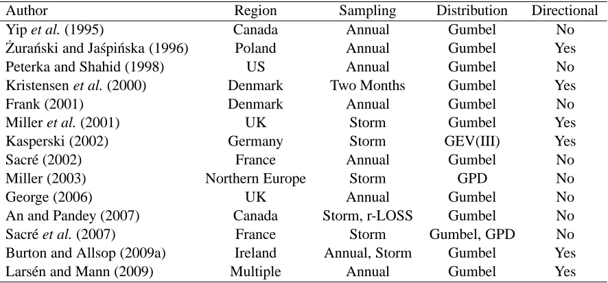
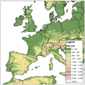
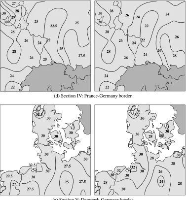
A preliminary study was carried out to investigate whether observed differences between 50-year return period wind speeds along national borders in Europe could be reduced by applying a simple, yet consistent, methodology and was published by Gatey and Miller (2007). Five examples of regions in Europe where differences exist between national bor-ders are identified in Figure 2.1, with each region shown in detail in Figure 2.2. The plot of each region has two portions; the left panel represents peer-reviewed 50-year return period wind speeds which have been published in conjunction with the methodology, and the right panel contains a comparison of the latest national building codes or national annexes (NAs) to Eurocode. Sources of the various 50-year return period wind speed values shown in Fig-ure 2.2 are summarised in Table 2.1. All 50-year return period wind speeds are 10-minute mean wind speeds at 10 m height for a roughness length of 0.05 m with the exception of the values for the UK. Both Miller et al. (2001) and BS6399-2 (based on Cook and Prior, 1987) provide hourly-mean wind speeds at 10 m height for a roughness length of 0.03 m,
I
II III IV
V
Figure 2.1: Regions of interest in Europe for the preliminary study
however, the combined correction from hourly-mean to 10-minute mean wind speed and a roughness length of 0.03 m to 0.05 m is generally taken as unity. Visual inspection suggests the German NA is based on Kasperski (2002) and the values for the French NA are possibly based on the methodology described by Sacr´e et al. (2007) who cite a reduced value (26 m/s) for a station on the French coast near the Belgian border which matches the French NA. Several discrepancies are noted here:
• 50-year return period wind speeds in France have been considerably reduced.
• The existing French values provided a better match to the Spanish code along the France-Spain border. Since the border between France and Spain follows the Pyren´ees, a true difference between wind speeds may exist.
• Differences have been reduced between the UK and France, however, there is still a considerable difference between the UK and both France and Belgium.
30 28
26
24
29
27
27
29
26
24
24
22
(a) Section I: France-Spain border
24 22 23
28 30
21 20
24
22
23
24 26
20
21
(b) Section II: English Channel (West)
20
21
30
26 26
28 20
22
23
24 26
24
26 25
24
23 24.5 27
27
29.5
24 24
21 20
(c) Section III: English Channel (East)
22.5 25 25 24 26 26 26 22.5 25 25 24 22 24 23 24 25
(d) Section IV: France-Germany border
30 30 30 27.5 27.5 27.5 25 25 25 30 30 22.5 25 25 21 22 23 30 30 30 27.5 27.5 27.5 25 25 25 30 30 24 27 27 24.5 29.5 25 24 24 27
(e) Section V: Denmark-Germany border
Figure 2.2: Comparison of European 50-year return period wind speed maps, published (left) and National Annexes (right)
Country Published Code
Spain – DB SE-AE 2009
• Large differences continue to exist between Denmark and Germany for 50-year return period wind speeds.
The majority of the NAs were unavailable or incomplete at the onset of the preliminary study, thus the study sought to reduce the discrepancies between the published values in Sections II through V. The NA values will provide additional comparison for the current study despite a lack of documentation regarding the underlying methodology for several nations.
Global surface summary of the day data was obtained from the National Climatic Data Cen-ter (NCDC), a division of the National Oceanic and Atmospheric Administration (NOAA). Basic quality control checks found that multiple years of data, at several stations, had to be omitted as a result of errors stemming from improper unit conversion. The data was processed using a basic traditional methodology for calculating 50-year return period wind speeds. Corrections were applied for anemometer height and the surface roughness rep-resentative of the site, thereby neglecting upstream effects, using the Deaves and Harris model (further discussed in Section 3.3.3). Annual maxima were extracted for each station and estimates with probability of exceedance of 0.02 were calculated using the Gumbel distribution (defined in Section 4.1). One of the major recommendations arising from the extreme value analysis in the preliminary study was for future investigations to consider methods for statistically identifying outliers, either spurious or relating to a longer return period. A method for statistically identifying outliers appearing in a dataset is presented in Section 4.3.
correlation across borders than various complex procedures being used individually by each nation. By identifying an ideal methodology for calculating 50-year return period wind speeds, estimates from the current study can be directly compared to Figure 2.2 to evaluate whether discrepancies arise from over- or under-estimation by a single nation or if a compromise can be established between existing values.
2.2
Surface Data
The dataset obtained for the current work consists of global hourly and synoptic observa-tions from the Integrated Surface Database (ISD), digital dataset DS-3505, managed by the NCDC. The ISD contains two fixed length and three variable length sections. The for-mer two are the control and mandatory data sections and the latter three are the additional data, remarks data and element quality data sections. The observations of interest are the mean wind speed and wind direction (mandatory data section), present weather identifiers and supplementary wind observations (additional data section) and observer comments (re-marks section). Full ISD documentation can be found in NCDC (2010).
The present weather identifiers and supplementary wind observations are recorded with varying temporal frequency. For example, the latter contains the recorded gust wind speed and/or gust wind direction, which are typically only recorded when the velocity exceeds a predetermined threshold (which may also vary temporally). In some instances the gust wind speeds may not be recorded at all. The remarks section occasionally contains addi-tional mean wind speed or gust wind speed measurements, as well as comments regarding thunderstorms or other relevant meteorological observations. Many of the remarks con-tained within the section follow the practices outlined in NOAA (2005).
hourly, continuous 10-minute mean, 10-minute mean before the hour and a 2-minute mean. Similarly, gust wind speeds may be block or continuous measurements. The directive of the World Meteorological Organization (WMO) mandates that anemometers should be lo-cated in open-country exposure and standard averaging times of 10-minutes and 3-seconds should be used for the mean and gust wind speeds respectively (WMO, 2008). As such, the mean and gust wind speeds documented in the ISD have been assumed to be a 10-minute mean wind speed recorded during the 10-minute period prior to the hour and a nominal 3-second gust wind speed observed throughout the hour. Measuring the 10-minute mean exclusively on the hour neglects 50-minutes of available wind observations. Continuous 10-minute mean wind speeds are thereby preferable, however, 10-10-minute mean wind speeds measured during the 10-minute period prior to the hour are available for the longest peri-ods. Observation networks such as the Automated Surface Observing System (ASOS) have now been recording continuously since 1998 and in the next decade will provide enough data to improve estimates of the true continuous 10-minute mean wind speeds in the US. Many stations currently report two times per hour, in these instances the observation near-est the hour is selected to maintain consistency throughout the record. When analysing a wind event it is important to consider the averaging time which will best represent the type of system or storm. Giving consideration to the characteristics of the European synoptic wind climate, the 10-minute mean wind speed is selected as the data type which best rep-resents the synoptic events of the region. The mean wind speed is also the most commonly available wind measurement thereby ensuring sufficient data for analysis.
Identifi-cation of these observations, and treating them in a consistent manner, is an important step in the overall methodology and is discussed further in Section 3.1.
2.3
Station Selection
The countries of interest located within Europe are Portugal, Spain, France, Ireland, UK, Belgium, Netherlands, Germany, Denmark, Czech Republic and Poland. For each WMO station present within the ISD, an inventory is available which indicates the available num-ber of observations per month on a annual basis. As a preliminary classification, all WMO stations within the countries of interest are queried and classified as primary, secondary or tertiary based on the number of complete years and number of observations per month. For the latter criteria, thresholds of 500 and 200 observations per month are selected as the minimum number of observations as they correspond to approximately a 28 day month containing 18 and 8 observations per day respectively. The criteria for the three classifi-cations are identified in Table 2.2. The inventory was originally parsed for observations commencing January 1970, however, few stations were found to have records in the period 1970-1972. As such, a consistent start date of 1973 was selected. Stations were mapped and hand-selected to ensure adequate spatial coverage where available, with preference given to stations of higher classification. The resulting 394 selected stations are shown in Figure 2.3 and a listing is provided in Appendix A. The entire data record is obtained from the ISD for each selected station and the relevant observations discussed in Section 2.2 are extracted for analysis.
Classification Criteria
Primary (I) Minimum 25 years of data and 500 observations/month Secondary (II) Minimum 25 years of data and 200 observations/month Tertiary (III) Minimum 15 years of data and 200 observations/month
Standardisation of Wind Speed Data
50-year return period wind speeds are to be representative of wind speeds recorded at 10 m height in open-country exposure. Standardising wind speed data provides a consistent framework for engineers to adjust standardised values to better suit the conditions at a spe-cific location. In the current work, standardisation is carried out in two steps. First, wind speed data is assessed by quality control algorithms, from which erroneous measurements and discontinuities in time histories are identified in a consistent manner. Second, wind speed measurements are modified to allow observations at different locations to be directly compared irrespective of site characteristics or sampling frequency. The latter process is commonly referred to as homogenisation. The following sections address quality con-trol algorithms, atmospheric boundary layer models, site exposure corrections and disjunct sampling.
3.1
Quality Control Measures
3.1.1
Background
When carrying out a statistical analysis of extremes, if left undetected spurious observations can greatly affect 50-year return period wind speed estimates. Methods for identifying such observations require attention, particularly for the current work where a subset of maxima is sought and errors are known to exist within the ISD. Quality control measures can also aid in determining if annual mean wind speeds are consistent over the entire data record or if considerable discontinuities exist. Identification of a shift may indicate changes of instrument location, height or local surroundings.
Documentation is occasionally available from meteorological agencies identifying dates of location or instrumentation changes, if unavailable, it is important to identify these changes to at least be aware that they exist.
model requires better detection of gradual changes and of breaks when the shift of the mean is less than the standard deviation.
Burton and Allsop (2009a) pre-process wind speed data in an attempt to identify individual observations for removal. Mean wind speeds greater than 20 m/s and three times greater than both adjacent mean hourly observations are classified as errors or thunderstorms, both of which are excluded from a synoptic climate analysis. For a number of regions in Europe of interest in the current work, the 50-year return period wind speed is less than 27 m/s, as was shown in Figure 2.2. A representative set of annual maxima will likely contain a subset of extremes which are less than 20 m/s, therefore, the maxima contained within the subset are not necessarily validated e.g. an annual maximum of 18 m/s is not considered by the pre-processing scheme. Such a situation is likely to arise, particularly when eval-uating directional extremes where maxima occurring from non-dominant wind directions are, in general, substantially lower than dominant wind directions. A lower threshold of 15 m/s suggested by Burton and Allsop (2009b) is likely more appropriate. Ideally, a method which can be applied to ensure the quality of every hourly wind observation is desired. The data can then be used to accurately derive the parent distribution if desired and, more im-portantly, ensures the validation of maxima regardless of the strength of the wind climate.
3.1.2
Global Quality Control Measures
Several global quality control measures of ranging complexity are considered. The most basic checks are for observations flagged as suspect or failing the ISD quality control de-scribed by Lott (2004). Other minor tests include physical limit checks identified by De-Gaetano (1997). The checks ensure the mean wind speed is less than the gust wind speed, the wind direction is a multiple of 10 and that measurements obtained during calm periods are properly transcribed.
The majority of observations within the ISD are reported on the hour, 10-minutes prior or 10-minutes after. Observations are prioritised in this order and, where multiple records exist, the highest ranking observation is selected resulting in a single observation for each hour. After culling the redundant observations, each station is tested against the tertiary classification outlined in Table 2.2 to ensure all stations meet the stated basic requirements. If a year of observations fail to meet this criterion, the year is removed from the record to ensure sufficient temporal resolution of observations throughout the year. Insufficient observations may be due to downtime associated with anemometer damage, measurement system replacement, freezing, or a site change. For several measurement stations in Ger-many, there are years where no records are reported at the expected reporting times, instead reporting was performed at 44 minutes past the hour. Thus, if a year is to be omitted due to insufficient measurements at the expected reporting times, a procedure is implemented to scan the previously parsed observations to evaluate whether there is a specific reporting minute which satisfies the minimum observation criterion.
by Domonkos (2011). The method, an adapted Caussinus-Mestre algorithm for networks of temperature series, is herein referred to as ACMANT. The PRODIGE and ACMANT methods are both recommended based on standardised benchmark tests carried out by Ven-ema et al. (2011). The ACMANT method contains two detection schemes, the main de-tection is based on annual means and summer-winter differences and secondary detection is used to identify short-term inhomogeneities. Domonkos (2011) notes that the radiation intensity affects temperature measurement and as a result, anomalies between time series during the summer naturally exhibit larger inhomogeneities than during the winter. Thus, the secondary detection scheme is based on monthly mean values and includes a harmonic annual cycle to account for the seasonal variation of inhomogeneity size. Theoretically, a similar cycle potentially exists for mean wind speed observations at mid- and upper-latitude locations as a result of the seasonal variation of surface roughness. In the winter months, deciduous plant species will shed their foliage and the surface is typically covered by snow. Under such conditions, wind speeds likely exhibit greater spatial correlation, re-ducing anomalies between time series, than during summer months when anemometers are affected by varying types and degrees of local vegetation. The correlation between monthly mean wind speeds as a function of month is shown for Bournemouth Airport, Hurn, UK and Caen-Carpiquet Airport, Carpiquet, FR in Figure 3.1 and indicates the assumption is appropriate.
The ACMANT method was carried out on six overlapping regions of approximately 100 stations as shown in Figure 3.2. For stations in overlapping regions, the detected change-points were found to be consistent between runs since the ACMANT method bases in-homogeneity detection on differences between stations whose series are well correlated. Figure 3.3 shows a typical time series and the identification of detected shifts by year.
Month
Correlation
1 2 3 4 5 6 7 8 9 10 11 12
0.4 0.6 0.8 1.0
Figure 3.1: Correlation of monthly mean wind speeds between Bournemouth Airport, UK (WMO 03862) and Caen-Carpiquet Airport, FR (WMO 07027)
the UK and Ireland was shifted by six months and the ACMANT method was carried out a second time. Between the original and modified time series, approximately 75 per-cent of the change-points were common within a couple months between the two datasets. Analysis of the change-points detected for winter and summer months between the two sets indicates a difference of only six percent, thus, even in a severe case where the annual cycle is assumed out of phase, the algorithm does not greatly impact the detected change-points for the current data.
Detected change-points were compared to what limited documentation on location, height and instrumentation changes could be found from the websites of various meteorologi-cal agencies, particularly Met ´Eireann, Koninklijk Nederlands Meteorologisch Instituut (KNMI) and Deutscher Wetterdienst (DWD); publications, Cappelan and Jorgensen (1999), Traup and Kruse (1996) and Verkaik (2001); and other available resources. Shifts verified to be related to a change of location or height are further considered in Section 3.3 for exposure correction.
Country Number of Stations Period Belgium 12 of 13 1996-1997 Germany 25 of 81 1999-2000 Ireland 10 of 12 1996-1998 Netherlands 16 of 16 1996-1997 Portugal 5 of 6 1997-2000 Table 3.1: Summary of conversion errors by country exhibiting possible conversion related errors are listed in Table 3.1.
3.1.3
Localised Quality Control Measures
The localised quality control algorithm is based on the excessive wind speed variability checks described by DeGaetano (1997). The general procedure is to extract a subset of data centred about an observation of interest and compare the maximum two hour wind speed difference in the subset, to the difference between the current observed wind speed and all other observations in the subset. Several criteria are to be met to identify a wind speed as suspect, including:
• The difference between the current observation and all observations in the subset must be greater than the maximum two hour difference in the subset.
• The difference between the current observation and all observations in the subset, neglecting the hour prior and after, must be greater than 7.7 m/s (15 kt).
• The current wind speed must be at least 3.1 m/s (6 kt) greater than the neighbouring hours.
PW Identifier Type Localised Quality Control Thunderstorm AU[1−9] Automated 2, 3 2
AW[1−4] Automated 18, 26, 42, 44, 46, 48, 58, 63, 66, 68, 73, 76, 80 : 97
26, 90 : 97
AY[1−2] Manual 8, 9 9
AZ[1−2] Automated 8, 9 9
MV[1−7] Manual 1, 2 1
MW[1−7] Manual 17, 18, 19, 25, 26, 27, 29, 59, 64, 65, 67, 69, 74, 75, 80 : 98
17, 19, 29, 91 : 98
Table 3.2: Present weather and thunderstorm identifiers
Several identifiers exist within the additional data section of the ISD which summarise the weather at the time of observation. The relevant present weather (PW) indicators for values related to strong showers and thunderstorms are shown in Table 3.2. The remarks section of the ISD often contains additional comments indicating the presence of thunderstorms. NOAA (2005) indicates a standard reporting style of TSBbbEee where b and e represent the hour relating to the start and end of a thunderstorm. Further investigation found that it is more common for a shorthand form of ‘thunderstorm’ to be reported. In general, the following word segments are capable of identifying the shorthand entries: STORM, THUN, T/ST, TSTO, TSTR. If an observation meets all rejection criteria, and one of the mentioned weather phenomena did not occur, the observation is removed.
The remarks section of the ISD often contains manual entries identifying the wind direc-tion, wind speed and, occasionally, gust wind speed measurements. Several of the entry formats follow those outlined in NOAA (2005), while other formats have been identified manually. Overall, eight different entries have been identified. Representing the wind direction, wind speed and gust wind speed as d, w and g respectively, the formats are:
dddww/ggKT, dddwwGggKT, dddwwwKT, dddwwKT, ddwwKT, MAX ggKT, MAXggKT
The quality control algorithms by DeGaetano (1997) were intended for complete hourly wind records, however, recommendations for application to a three-hour sampling interval were provided. In the current work, three assumptions regarding the average number of observations per day, calculated by month, have been made. Months where a median of 18 observations per day or greater exist, are treated in the same manner as those having 24 hourly observations. A median of 9−17 observations per day typically indicated ob-servations were being recorded during the daily operational hours of a site. Lastly, a three hour sampling interval was assumed if the median number of observations per day was between 6.5 and 9. Table 3.3 contains the temporal interval considered in the local qual-ity control subset, the corresponding subset size and the minimum number of observations in the subset required for the localised quality control check to be applied to the current observation. The subset interval for hourly and three-hour sampling intervals are provided by DeGaetano (1997). The minimum subset size is considered here to ensure sufficient measurements are present to adequately evaluate the current observation. The criteria for measurements occurring throughout operational hours is defined in relation to the criteria for the hourly and three-hour sampling intervals.
The current procedure relies on accurate and complete records of PW identifiers. In the instance where the PW identifiers are incomplete, a short duration high-intensity wind (HIW) event may be rejected if it was not recorded that an associated incident, such as a thunderstorm, was present. Given the focus on synoptic winds, the potential rejection of a measurement associated with a HIW event is not of great concern as the events are typ-ically driven by convective mechanisms. In addition, it is possible for two closely spaced
Median Obs./Day Subset Interval Max. Subset Size Min. Subset Size 18≤ −11.5 to+12.5 hours 24 16
9−17 −18.5 to+21.5 hours 14-39 14 6.5−9 −18.5 to+21.5 hours 14 11
Observations Failing Local Quality Control
Number of Stations
0 10 20 30 40 50
0 25 50 75 100 125 150
Figure 3.4: Distribution of observations failing local quality control checks
erroneous measurements to shelter one another from identification as shown by DeGaetano (1997). Overall, it was found that the average number of rejected observations per station was 9 with a maximum of 52 for Sniezka, Poland. The distribution of rejected observations per station is shown in Figure 3.4. The localised quality control method described here to validate individual wind speed measurements is an important analysis used to identify spurious observations. The method can be applied to an entire time history or to a set of extracted maxima, provided the required temporally adjacent observations are available.
3.1.4
Thunderstorm Identification
a thunderstorm ended during an observation hour, a one hour event could affect the local wind climate, and associated measurements, for up to two or three hours prior or after the recorded observation. Thus, the adjacent two hours, both before and after a reported thun-derstorm hour are extracted as contaminated synoptic observations and archived for future investigation. The weather indicators relevant to strictly thunderstorms are listed in Table 3.2.
The criteria for reporting a thunderstorm will often vary between national meteorological organisations. A thunderstorm classification may be based on hearing thunder or seeing lightning, however, there is no guarantee that the wind speed recorded is representative of a thunderstorm wind. Future algorithms to identify thunderstorms could benefit by giving consideration to the temperature and the ratio of gust to mean wind speed at a location, provided all three measurements are available with sufficient temporal resolution. Such a scheme would allow thunderstorms to be detected in the absence of present weather identifiers and to verify the reverse.
3.2
Atmospheric Boundary Layer
3.2.1
Background
surface layer, the law of the wall indicates that the velocity scales as a function of height and surface roughness, which holds for approximately the bottom 10 percent of the ABL (Simiu and Scanlan, 1996). The upper or outer layer of the ABL is defined by the veloc-ity defect law which is a function of the velocveloc-ity at the top of the boundary layer and the height of the boundary layer. An intermediate layer between the surface and outer lay-ers is assumed to exist in which both laylay-ers overlap. Blackadar and Tennekes (1968) use asymptotic similarity theory (AST) to equate these two layers from which the log-law and geostrophic drag law equations are derived. The log-law for neutrally stable conditions is commonly expressed as
u(z)= u∗ κ ln
z z0
!
(3.1)
near the surface, where u(z) is the mean velocity at height z, u∗is the friction velocity,κis the von Karman constant and z0 is the roughness length. The geostrophic wind speed (G)
is calculated from the geostrophic drag law as
G= u∗ κ
s "
ln u∗
f z0
!
−A
#2
+B2 (3.2)
where f is the Coriolis parameter, and, A and B are generally treated as dimensionless parameters, although they have been identified as functions of stability and boundary layer height (Zilitinkevich and Esau, 2002). A summary of values selected by researchers to represent the two parameters in Equation 3.2 is provided by Zilitinkevich (1989)
In the field of wind engineering, the power-law was originally used to model the mean wind profile within the ABL due to its simplicity and improved estimates away from the surface. The power-law is expressed as
u(z)=ure f
z zre f
!1/α
where ure f is a wind speed at reference height zre f andαis an empirically derived exponent dependant upon exposure. The Engineering Sciences Data Unit (ESDU) standard for over 30 years is a semi-empirical boundary layer model proposed by Deaves and Harris (1978). The model is based on the assumption of neutral steady-state conditions and AST. Em-pirical estimates are used to determine four theoretically derived constants which yield a parabolic profile for a majority of the boundary layer. The mean wind profile of the Deaves and Harris model is expressed as
u(z)= u∗ κ
ln
z z0
!
+5.75 z
zh
!
−1.878 z
zh
!2
−1.333 z
zh
!3
+0.25 z
zh
!4
(3.4)
where zhis the height of the boundary layer. Despite its widespread acceptance in the wind engineering community, the model has never gained popularity in other fields due to a lack of publishing in peer-reviewed journals outside of the community.
Gryning et al. (2007) recently proposed a boundary layer model which has been validated using data obtained from several tall towers. The model contains three separate wind pro-files corresponding to the neutral, stable or unstable conditions. In addition, the model considers length scales appropriate for the surface, middle and upper layers of the bound-ary layer. The model was validated against 160 m and 250 m towers by Gryning et al. (2007) and, a 300 m tower and the Leipzig, Germany wind profile up to 900 m by Pe˜na
et al. (2010).
Observations from the Leipzig wind profile as re-examined by Lettau (1950), along with wind profile fits from the aforementioned models, are shown in Figure 3.5. The fits are calculated using u∗ = 0.65 m/s from Lettau (1950) and z0 = 0.1 m as determined by Pe˜na
et al. (2010). The exponent for the power-law is estimated from
α= 1
ln(10/z0)
where the wind speed at 850 m is used as the reference value in Equation 3.3. Considering the uncertainty associated with the measurements obtained from the 28 pilot balloons used to form the Leipzig wind profile, the majority of ABL models perform quite well with the exception of the log-law which, as given by Equation 3.1, is only valid near the surface. Due to the more extensive and transparent validation techniques performed by Gryning
et al. (2007) and Pe˜na et al. (2010), and the flexibility of the model to allow for potential
consideration of stable and unstable boundary layers, the model proposed by Gryning et al. (2007) is selected for modelling the mean wind profile in the current work.
3.2.2
Gryning ABL Model
The ABL profile model proposed by Gryning et al. (2007), herein referred to as the Gryning ABL model, is based on the assumption that there are three components which contribute to the length scale, one each for the surface, middle and upper layers of the ABL. Length scales in the surface layer appropriately scale with height, while those in the middle layer are assumed to be dependant on stability. The influence of the length scale in the upper layer is thought to be relatively unknown and as a result, the length scale is assumed to decrease to zero as a function of the distance from the top of the boundary layer, similar to scaling in the surface layer. The mean wind profile under neutral conditions is given by Gryning et al. (2007) as
u(z)= u∗0 κ
"
ln z
z0
!
+ z
LM −
z zh
z
2LM
!#
(3.6)
U [m/s]
z
[m]
6 8 10 12 14 16 18 20
0 200 400 600 800 1000
Data Gryning
Deaves and Harris Log−law Power−law
Figure 3.5: Fits of various wind profiles to the Leipzig wind profile analysed by Gryning et al. (2007) and is expressed as
u∗0
f LM
=−2 ln u∗0
f z0
!
+55. (3.7)
The boundary layer height can be approximated from the Rossby-Montgomery formula, given as
zh ≈cu∗0/f (3.8)
3.3
Heterogeneous Exposure Correction
3.3.1
Background
The majority of stations providing the greatest temporal duration of measurements are typ-ically located on airfields. Anemometers located on airfields are generally sited in near open-country exposure, however, after initial placement local disturbances may arise due to the expansion of airport facilities or hangers. In addition, airfields are typically placed sufficiently far from urban or suburban centres, although urban sprawl may result in reduced fetch between the two regions. Correction of observed wind speeds (u) to standardised val-ues (uB) allows for the direct comparison of final predicted wind speeds. The ratio of the observed to corrected value is referred to as the correction factor. For the current work, observed values are standardised to the WMO standard height (10 m) and open-country ex-posure (z0 = 0.05 m). The effects of heterogeneous exposure can be corrected to standard
open-country exposure by several different approaches of ranging complexity.
The combined effects of upstream heterogeneous exposure can be summarised in terms of an effective roughness length at the site. The effective roughness length can be calculated from the wind profile, turbulence intensity of the wind, or gustiness at a site. Barthelmie
et al. (1993) compared several of these methods, including determination of the roughness
selected to represent the ratio of the standard deviation of the wind to the friction velocity which likely requires additional consideration of the impact of the transfer functions of the measurement instruments on the wind spectrum.
By deriving roughness lengths from wind measurements, one can easily evaluate changes of roughness over time or identify periods potentially affected by local sheltering. Wind profile-derived roughness lengths are ideal, however, in practice the availability of such in-formation is limited to locations where towers are instrumented at multiple heights. Rough-ness lengths derived from the standard deviation of the wind, or turbulence intensity, require measurements obtained with a sampling frequency which is much greater than the hourly measurements obtained for the current work. Stations with sufficient data to perform such an analysis are available from ASOS for the US, whereas a Europe-wide equivalent is cur-rently unavailable. Roughness lengths can be derived from gustiness if sufficient gust wind speed data is available for a specified location using methods proposed by Wieringa (1973, 1976) and Beljaars (1987). Application of the latter to ASOS data is discussed by Masters
et al. (2010).
to evaluate the accuracy.
Preliminary investigation found that the majority of stations in the current work provide insufficient gust wind speed observations at high mean wind speeds in the non-dominant wind directions. In addition, documentation defining the characteristics of existing measur-ing chains is largely unavailable. Thus, to maintain the ideology that a consistent method-ology is an important factor in the estimation of 50-year return period wind speeds, the only alternative for the current work is to calculate a correction factor based on land use land cover (LULC) information. A simple approach to correcting exposure at a site to the reference height and roughness length considers only the height of the anemometer and roughness length at the site. However, it is known that changes in upstream roughness can have a significant impact on the wind profile. Letchford et al. (2001) have shown that up-stream roughness effects can be significant, thus, correcting by both direction and distance is desirable. More sophisticated models exist which calculate the effects of non-uniform surface roughness on the boundary layer by both distance and direction.
shown by Cook (1997) to greatly reduce the directional variance in comparison to assum-ing uniform exposure; reductions in variance were not as significant for sites affected by topography.
TL models focus on two regions, a lower surface layer and an upper layer. The height at which these two regions meet is identified as the mesolevel or blending height (Wieringa, 1976, 1986). TL models consider the effects of the local roughness within the surface layer and the mesoscale roughness, which is representative of a larger region, within the upper or macrolevel. Through consideration of these roughness effects, model equations, and a given height, the resulting wind speed at a particular location can be determined.
The TL model of Wieringa (1986) can be used to predict the wind speed profile over multi-ple changes of roughness. An approximation to the area within which the roughness length contributes to the surface flux was incorporated into the model by Verkaik (2003). The combination of the TL model proposed by Wieringa (1986) and the footprint approxima-tion of Verkaik (2003) is here referred to as the Hydra TL model. Verkaik (2003) reported relative errors in wind speed predictions of 10 to 15 percent but expected better results after revision of the model. Many of the stations for which measured and estimated wind speeds were compared, were located on the coast and some large distance inland. The model was validated by using observations from multiple locations to calculate a macrolevel windfield, then interpolating the wind speed to a separate site and comparing the estimate to recorded data.
due to the change in wind direction, were related to the effects of nearby woodland. Simu-lating this change of roughness using the Deaves and Harris model, Letchford et al. (2001) found that the model typically overestimated the speed up associated with a change from a rough to smooth surface, predominantly with mean wind speeds as opposed to gusts.
In this section, the Deaves and Harris IBL and the Hydra TL models as proposed by Cook (1985) and Verkaik (2003), respectively, are summarised briefly. An alternative model is proposed which combines the concept of the TL model with the Gryning ABL wind pro-file. For several stations in the Netherlands, correction factors are calculated for 30-degree sectors from gustiness- and LULC-derived effective roughness length estimates using each of the three correction methods. The differences between the gustiness- and LULC-derived correction factors are calculated and compared across the three models.
3.3.2
Methodology
the majority of the KNMI observation network since converting to automatic weather sta-tions in the 1990’s (Verkaik, 2000). Through application of Beljaars’ gustiness model to the observations at 13 stations, effective roughness lengths are calculated by direction. The effective roughness lengths are calculated for 30-degree sectors having a minimum of 30 gust factor values with a minimum mean wind speed of 10 m/s. For each wind direction satisfying this criterion, the log-average of the estimated effective roughness lengths for the sector is calculated. This method provides a single effective roughness length for each direction and is applied for each measurement chain identified at the location. If diff er-ent measuremer-ent chains were consecutively employed at a consister-ent mast location, then the weighted average of the effective roughness length determined from the measurement chains was calculated. This final step ensures a single effective roughness length is evalu-ated for each direction and mast location at the station.
To calculate the LULC-derived correction factors, a geographic information systems (GIS) tool has been developed to sample a LULC database by distance and direction from a site of interest. The Coordinate Information on the Environment (CORINE) LULC database is a Europe-wide 44 class LULC raster database developed by the European Environment Agency (EEA) and is selected for the current work. The database was created by compil-ing LULC databases from individual countries uscompil-ing a common framework. In theory, the common framework should provide fairly consistent results. The version of the CORINE database used in this study has a pixel resolution of 100 m by 100 m where each pixel con-tains an integer value representing one of the 44 LULC classes. Taking into consideration both the various land cover nomenclature set out by the CORINE documentation (Bossard
et al., 2000) and a review of roughness lengths by Wieringa (1993), roughness lengths are
assigned to the 44 LULC classes as shown in Table 3.4. Gatey and Miller (2007) and Sacr´e
et al. (2007) also use the CORINE LULC database to assign roughness lengths. A few
z0[m] CORINE LULC Classes
0.003 331, 332, 335, 511, 512, 521, 522, 523 0.005 333, 422, 423
0.010 412, 421 0.034 142, 231
0.05 124, 213, 321, 322, 334, 411 0.06 211, 212
0.10 121, 132
0.15 211, 222, 223, 241, 242, 243 0.25 131, 133, 323
0.3 244
0.5 122, 123, 141, 324 0.6 112
1.0 111,331,312,313
Table 3.4: LULC roughness assignments
values overall show good agreement. The selected CORINE database is for the year 2000, which is the only version to include the UK. Given the database is representative of a single year, the current analysis will not account for any changes of roughness over time.
Figure 3.6: CORINE LULC and sampling grid (meso- and local-scale) for Den Helger Airport, De Kooy, NL (WMO 06235)
3.3.3
Deaves and Harris IBL Model
Parameters known as S-factors are utilized to account for several aspects including height (SZ), site exposure (SE) and fetch (SX). It is the net effect of these factors which allows for manipulation of wind speed data. The mean wind speed as calculated using the Deaves and Harris S-Factors is given by the equation
u=SX{n−m}...SX{c−b}SX{b−a}SZ{a}SE{a}uB (3.9)
where u is the mean wind speed at anemometer height z, uB is the basic wind speed at height zBfor roughness length z0,B, n denotes the furthest upstream roughness, and a is the site roughness. The S-factors as given by Cook (1985) are determined from the following expressions
Height Factor
SZ =
ln(z/z0)+5.75(z/zh,0)−1.875(z/zh,0)2−4(z/zh,0)3/3+(z/zh,0)4/4
ln(10/z0)
where zh,0is the height of the ABL for roughness length z0.
Exposure Factor
SE =
ln(zh,B/z0,B+2.79ln(10/z0)
ln(zh,0/z0+2.79ln(10/z0,B)
(3.11)
where zh,Bis the height of ABL for the basic roughness.
Fetch Factor
SX{j→i}=
"
1− ln(z0,j/z0,i) 0.42+ln m0
#
ln(10/z0,i) ln(10/z0,j)
SE,j
SE,i
(3.12)
where j and i denote the upstream and downstream profiles respectively, and m0 is
calcu-lated as
m0 =0.32X/z0,i(ln m0−1) (3.13)
where X refers to the distance of the site downstream of the change of roughness.
3.3.4
Hydra TL Model
Prior to the calculation of wind speeds, the Hydra model first approximates a local and mesoscale footprint. For each cell, the drag coefficient is calculated from
Cd =
κ
ln(zbh/zo,e f f)
(3.14)
where zbh is the blending height chosen by Wieringa (1986) to be 60 m and z0,e f f is the log-averaged effective roughness length of the cell. The average drag coefficient for each 30-degree sector is then expressed as
C′d = ΣW(x/D)Cd
ΣW(x/D) (3.15)
where weighted averages are calculated based on the distance of a cell from the site as
W(x,D)=exp(−x/D) (3.16)
where x is the distance from the site and D is given by Verkaik (2003) to be 600 m and 3000 m for local and meso-scale footprints respectively.
Two differences exist between the calculation of the effective roughness lengths in the cur-rent work and the Hydra model:
• Verkaik (2003) proposed 5-degree wide sectors for which Cd′ is smoothed using a weighted moving average considering three sectors on either side of the centre sector. In the current work, all sectors are 30-degrees and are not smoothed as the resolution of the LULC grid is significantly more coarse.
Once an effective drag coefficient has been calculated for the local and mesoscale foot-prints, the effective roughness lengths are solved for. From the local effective surface roughness, the mesolevel wind is calculated as
umeso =u×
"ln(z
bh/z′o,s) ln(z/z′
o,s)
#
(3.17)
where u is the surface wind speed at anemometer height z and z′
o,s is the local effective roughness length. Incorporating the mesoscale effective roughness length (z′
o,m) the friction velocity is given by
u∗,m=κumeso/ln(zbh/z′o,m) (3.18)
Once the friction velocity is known, the macroscale wind can be calculated as
Umacro =(u∗/κ)
"
ln u∗
f zo,m
!
−A
#
(3.19)
where A= 1.9 and B=4.5 for neutral conditions. By reversing this process and assuming that z′
o,m = z′o,s = 0.05 m and z = 10 m, the basic wind speed can be calculated and an appropriate correction factor determined.