ABSTRACT
NING, BO. Analyze the Effect of Oil Shocks on the U.S. Economy in a Time-Varying-Parameter Structural VAR Framework. (Under the direction of Atsushi Inoue.)
This thesis applies a time-varying-parameter (TVP) structural VAR model with Markov
chain Monte Carlo methods to analyze the effect of oil shocks on the U.S. economy. The
thesis reports clear evidence of opposite tendency of shocks - supply shock gradually
decreasing and oil-specific demand shock gradually increasing - since the 1970s. This
evidence suggests Kilian’s view on considering the importance of demand shock instead
of supply shock is partly right. Also, six events that may affect oil shocks are selected
and the structural impulse responses are drawn correspondingly to each event. The plots
explain which of the three factors - oil production, real economic activity and price of oil
- is the impetus to cause the responses to change. Furthermore, this thesis compares the
TVP structural VAR model to a time-invariant-parameter structural VAR and a
con-ventional structural VAR models. The comparison illustrates that the TVP structural
VAR model has the following advantages: it could draw structural impulse responses for
different years and analyze the time-varying effect of each selected event and could adjust
© Copyright 2013 by Bo Ning
Analyze the Effect of Oil Shocks on the U.S. Economy in a Time-Varying-Parameter Structural VAR Framework
by Bo Ning
A thesis submitted to the Graduate Faculty of North Carolina State University
in partial fulfillment of the requirements for the Degree of
Master of Science
Economics
Raleigh, North Carolina
2013
APPROVED BY:
Denis Pelletier Nora Traum
Atsushi Inoue
DEDICATION
BIOGRAPHY
The author was born in Chingtechen city, Chianghsi province, China. He is pursuing both
economics and statistics master degree in NC state university since 2011. During master
in economics, he selected econometrics as a main concentration. Under his professor and
ACKNOWLEDGEMENTS
I would like to express my greatest gratitude to the people who have helped and
sup-ported me throughout my master studies in Economics. I am grateful to Professor Atsushi
Inoue for his continuous support for the thesis, from initial advice and contacts in the
early stages of conceptual inception and through ongoing advice and encouragement to
this day. Without his support and encouragement, this thesis cannot be even finished.
I wish to thank my parents for their undivided support and interest who inspired me
and encouraged me to go my own way, without whom I would be unable to complete my
TABLE OF CONTENTS
LIST OF TABLES . . . vi
LIST OF FIGURES . . . vii
Chapter 1 Introduction . . . 1
Chapter 2 Literature Survey . . . 4
2.1 Literature survey on oil shocks impact to economy . . . 4
2.2 Literature survey on time-series model estimations . . . 6
Chapter 3 Data, Model and Estimation Methods . . . 11
3.1 Time-series model framework . . . 12
3.2 The Time-Varying-Parameter model . . . 12
3.3 The time invariant parameter model . . . 16
Chapter 4 Empirical results of the Time-Varying-Parameter model . . . 18
Chapter 5 Model comparison and convergence diagnosis . . . 26
5.1 The conventional structural VAR model . . . 26
5.2 The time invariant parameter structural VAR model and model comparison 27 5.3 Sensitivity analysis . . . 29
5.4 Convergence diagnostics for hyperparameters and volatilities . . . 29
Chapter 6 Conclusion . . . 32
REFERENCES . . . 34
APPENDICES . . . 38
Appendix A Derive posteriors of BT, DT and ΣT in the TVP model . . . 39
Appendix B Derive posteriors of DT and ΣT in the time invariant parameter model . . . 43
Appendix C Plots of structural impulse responses in TVP model . . . 45
LIST OF TABLES
Table 5.1 Summary of the distribution of the IFs for different sets of parameters. 31
LIST OF FIGURES
Figure 4.1 Posterior mean, the standard deviation of residuals for shocks . . . . 19
Figure 5.1 Structural impulse response of the conventional structural VAR model 27 Figure 5.2 Structural impulse response of the time invariant VAR model . . . . 28 Figure 5.3 Convergence diagnostics for hyperparameters and volatilites. . . 30
Chapter 1
Introduction
A large body of research suggests a relationship exists between oil price shocks and the
macroeconomy, especially after the beginning of the 1970s when the oil-price increases
coincided with the stagnation of the US economy. Hamilton’s early work in 1983 and
Burbidge and Harrison (1984) suggested the oil price Granger-cause macroeconomic
vari-ables. Along with their research, several studies including Santini (1985), Daniel (1997),
Muellbauer and Nunziata (2001), Barsky and Kilian (2001, 2004), also found the impact
of oil price to the macroeconomy cannot be ignored based on increasing datasets and
events that affect oil shocks. Other works such as Pindyck (1980), Mork (1989), Lee, Ni
and Ratti (1994), Mork and Olsen (1994), Ferderer (1996), Hooker (1996), Balke et al.
(1999), and Hamilton (2003) considered the “asymmetries phenomenon” of oil price: the
effect of increasing oil price on retarding the US economy is larger than the effect of
decreasing oil price on stimulating it. More recently, Kilian (2009) specified the demand
and supply shocks, and he concluded that the demand shock plays a more important role
on predicting the macroeconomy than the supply shock.
price shocks, which may help identify some unobserved shocks. Methods, such as
boot-strap, Kalman-filter, classical minimal distance estimators, simulated maximum
likeli-hood, Markov chain Monte Carlo algorithm and marginal likelilikeli-hood, and models such as
stochastic volatility model (i.e., GARCH and ARCH), state space models and Bayesian
vector autoregression models have been applied in oil-price shocks models by previous
researchers.
Bayesian methods are becoming increasingly popular in empirical macroeconomics.
Lit-terman (1986), Todd (1984), DeJong et al. (1993), Ingram et al. (1994), Del Negro et
al. (2004,2009) and Ghent (2009) are the representatives to apply Bayesian methods
in estimating a trivariate macro model of GDP, inflation and interest rate. Most
re-cently, Jo (2012) applies the Bayesian method to a time-varying volatility VAR model
to measure the negative relationship between oil price uncertainty and world industrial
production. The idea in this paper is to apply Bayesian methods to an oil-price model
to find new evidence on the oil price shock and macroeconomy relationship. Based on
this idea, this thesis applies Primiceri’s (2005) time-varying-parameter (TVP) model to
re-estimate Kilian’s (2009) model with three factors of shocks: oil supply, aggregate
de-mand and oil-specific dede-mand. Also, this paper compared this model with a short-run
restricted structural VAR model and a time invariant parameter structural VAR model.
After making the comparison, the TVP model gives a more accurate view on performing
shocks. More explicitly, I found that the oil-specific demand shock became more volatile
after 1985 and in the meantime, the oil supply shocks has been decreasing to flat. This
confirms Kilian’s viewpoint that the oil-specific demand shock plays a more important
role in predicting the macroeconomy in recent years, and this finding also disagrees with
Kilian’s other viewpoint that earlier researchers got it wrong in focusing on the oil-price
why earlier researchers took importance on it. Besides drawing the volatility of shocks,
this paper also draws the structural impulse response functions for selected events such as
the Embargo that happened in 1973, and compares the time-varying effects by drawing
the difference between structural impulse responses after the event and before the event
happened.
Furthermore, this thesis compares the TVP model with the conventional time invariant
parameter structural VAR model, where the time invariant parameter model is simply
setting all the time-varying parameters to a fixed value. After comparing structural
im-pulse responses of each model, it appears the TVP model gives a smaller shock range
than the conventional model. Also, the time invariant parameter model gives more
per-sistent shocks, even after 20 months.
This thesis is different from Jo (2012) though they are both applying a time-varying
VAR model. First, Jo focused on measuring the effects on oil price shocks to economic
activity, but this thesis pays attention to three variables: price of oil, economic activity
and oil production. Furthermore, this thesis has different time-varying models, and thus
the Gibbs sampling process is different from Jo’s. Finally, Jo compared her method to
Elder et al.’s (2010) GARCH model, but this thesis compares with Kilian‘s model.
The thesis is organized as follows: section 2 discusses the literature on oil-price shock and
Bayesian structural VAR models. Section 3 presents key steps of the time varying and
invariant structural VAR model. Section 4 illustrates empirical results of the implication
to oil-price shocks. Section 5 compares with models and does a convergence diagnose for
Chapter 2
Literature Survey
This thesis is mainly focused on applying time-varying-parameter VAR models to
esti-mate the effect of oil shocks on the macroeconomy. Following this topic, I searched most
of the literature on the effects of oil price shock on the economy and VAR models. By
doing this, I would like to separate this part into two parts. The first part summarizes
some important literature on oil-price shocks, and the second searches the literature on
model estimation.
2.1
Literature survey on oil shocks impact to
econ-omy
Since the 1970s, the phenomenon of stagnating of U.S. macroeconomics performance
coincided with the increasing of oil price interests lots of researchers to argue whether
there is a relationship between them or not. Until now, it seems that there still did not
decades. Hamilton is one of the famous researchers who began to verify the relationship
in the early 1980s, he tested the relationship between oil prices and output. And the test
showed there is no significance to reject this relationship in 1983. Burbidge and Harrison
(1984) also found the oil price shocks increase could cause macroeconomics variables to
change, though it is not necessary to do with explaining the cause of stagflation that
happened in early 1970s. But this conclusion was questioned by Hooker (1996) soon.
Hooker argued Hamilton’s (1983) conclusion is made by using post-war and pre-OPEC
period data, the period when there were few oil price decrease observations. Meantime, he
also applied the Granger causality method by using extended data, and there no longer
shows strong evidence on oil prices and U.S. macroeconomics variables (such as GDP,
unemployment rate and industrial production) relationship after 1973. He also proposed
a new idea that there existed a structural break in 1973. After 1973, oil shocks become
endogenous to macroeconomics indicator variables. Furthermore, he found an
asymmet-rical phenomenon between the effects of oil price increases and decreases. This finding
shed a light on later works that people began to consider oil shock both in increasing and
decreasing situation. After Hooker’s paper, extended database supports a more mature
platform to investigate oil price shock and macroeconomics variables relationship. Barsky
and Killian, two other notable researchers on oil price shock, believed oil price shocks not
only interfered with the macroeconomy but associated with major macroeconomics
re-cessions, and the association is less than perfect (Barsky and Kilian, 2004). Barsky et al.
(2001) pointed out that oil price increases could result in 1970’s stagflation through
Nel-son’s (1998) “sluggish inflation”. To be more precise, Barsky and Kilian (2004) explained
how oil price shocks affect inflation, economic growth and recessions. Putting conflicts
on macroeconomy performance and oil price shocks causality aside, some literature
more dominant in influencing the macroeconomy: price increasing or price decreasing, oil
supply shock or oil demand shock. Lots of work has been done to judge the contribution
of oil price changes on the macroeonomy: the represent active works included Pindyck
(1980), Mork (1989), Lee, Ni and Ratti (1994), Mork and Olsen (1994), Ferderer (1996),
Balke, Brown and Y¨ucel (1999) and Hamilton (2003). The common phenomenon they
found is that there exists some asymmetric effect: oil price increase on retarding U.S.
economy is more obvious than a decrease on stimulating it: this may be caused by oil
price volatility (Ferderer (1996)). Kilian (2008a, 2009) separated oil shock to demand
and supply shocks. He considered the demand side of oil is the right side of explaining
oil price shock to macroeconomy, and any analysis focus on supply side is misplaced. My
thesis uses some of Kilian’s conclusions, and more details of his work will be discussed in
the following context. Jo (2012) focuses on analyzing oil price shock to economic activity:
she found that due to the uncertainty of oil price, there has been significant influence on
global real economic activity (i.e., world industrial production).
2.2
Literature survey on time-series model
estima-tions
Macroeconomic variables, such as GDP, unemployment rate and CPI, are often called
time-series variables due to the fact that they are correlated with their own lags. Based on
the nature of these variables, traditional models and estimation methods do not consider
time series correlation so that they cannot be applied directly. There are many new
is a vector autoregression (VAR) model. More advanced models are, for instance,
struc-tural VAR model with short-run and long-run restrictions, stochastic volatility model,
autoregressive conditional heteroskedasticity (ARCH) model (Engle, 1982) and
gener-alized autoregressive conditional heteroskedasticity (GARCH) model (Bollerslev, 1986
and Elder et al., 2010). Both of these models allow variables to respond with their own
lags. Following these models, new estimation techniques were also developed. Besides
traditional techniques such as OLS, GLS, GMM, Andrew Harvey (1990) introduced the
Kalman-Filter method to structural time series model, Berkowitz and Kilian (2000)
sum-marized bootstrap methods, Ruge-Murcia (2012) applied simulated moments methods to
DSGE model, Gourieroux and Renault (1993) comes out indirect inference method, Sims
and Zha (1998, 1999) devoted lots of research on Bayesian VAR methods.
Let’s concentrate on the literature on models related to this thesis. I will separate the topic
to traditional VAR and Bayesian VAR estimations. The frenquentist normally dealing
with VAR models by using statistics inference. Hamilton (1983), Hook (1996), Bernanke
et al. (1997), Kilian (2009), Nathan S. Balke et al. (1999) and Wu et al. (2011) are the
representatives. Hook carried on Hamilton‘s research, as introduced in section 2.1,
estab-lished VAR models and conducted granger causality on examining the cause of oil price
shock to macroeconomy. He found oil price shocks no longer Granger cause
macroeo-nomic variables. Bernanke, Gelter and Watson (1997) (“BGW”) formed a five-variable
(include GDP, GDP deflator, CPI, Federal funds rate and the Hamilton oil price variable)
quasi-VAR with 7 lags. They concluded it was the monetary policy, not oil prices, that
caused the economy change during 1965-1995 period. Kilian borrowed a structural VAR
with short-run restriction model to identify demand and supply shock in oil prices. Balke,
Brown and Y¨ucel follows BGW’s model; they focus on the asymmetric effects of negative
com-bine “narrative and quantitative approaches” to make oil price shocks truly exogenous,
and they came up an interesting result: “Traditional VAR-based measures of oil-price
shocks exhibit two recurrent weaknesses: endogeneity and predictability.” Fern´
andez-Villaverde et al. (2007) reiterated that though VAR could identify economic shocks and
impulse-response functions in most cases, but under a not complete and partly trusted
model, it is recommended to apply likelihood function-based methods. As Wu et al. and
Fern´andez-Villaverde et al. found, VAR estimation in the frenquentist way is not always
perfect. When dealing with oil-price shocks contained with endogenous movements, the
estimates of the effects of oil shocks would be biased; this weakness is called endogeneity.
Another weakness is named as predictability. When oil price changes are anticipated by
private agents well in advance, the changes cannot be treated as “shocks.” Due to these
reasons, there urges another methods to come out.
Bayesian, a substitution method to traditional VAR, becomes increasingly popular in
macroeconomics applications due to some obvious advantages. At first, it avoids
tra-ditional VAR model’s identification problem. Bayesian methods acquire to identify a
complete distributions for all parameters (Fern´andez et al., 2007). Due to complete
dis-tributions are needed, forecasting outcomes on macroeconomy would be more realistic
than generated by other approaches (Litterman, 1986). Furthermore, it is convenient to
adjust models through prior changes. Also, the Bayesian approach has advantages to
solve high dimension models. Researchers such as Sims and Zha did a lot of work in
fitting Bayesian methods to multivariate models (i.e. the VAR model). Sims and Zha
(1998, 1999) are the main contributions in applying Bayesian ideas to structural VAR
(or BVAR): they help to identify the likelihood and the error band of impulse response
functions, they also help to select reasonable prior distribution. Jo (2012) suggested there
that the model allows the volatility process to have its own innovation term, but a
tra-ditional model (i.e., GARCH model) can only treat the volatility process as a function
of changes in the level and past volatility.
But to choose an unreasonable prior may result in unrealistic estimation and could
be-come a disadvantage for Bayesian analysis, and there is always existed conflict in
se-lecting “reasonable” priors. The Minnesota prior is one of the commonly used priors.
Litterman (1986), Todd (1984) and Ingram and Whiteman (1994) choose this prior to
predict macroeconomic variables. Besides the Minnesota prior, DeJong and Whiteman
(1993), Del Negro and Schorfheide (2004, 2009), Ghent (2009), Ingram and Whiteman
(1994) preferred priors from general equilibrium models on VAR models. Del Negro and
Schorfheide applied VAR with a DSGE prior to a trivariate model, which includes GDP
growth, inflation and interest rate. They concluded the DSGE prior works better than the
Minnesota prior due to two reasons: it allows for analysis interventions in policy shocks,
and could be used to predict permanent change effect of policy rules. Ghrent compared
four types in forecasting of RBC models with DSGE-VAR application. The outcomes
of four models are similar and the basic RBC model with indivisible labor works better
than others. Besides the Minnesota prior and general equilibrium prior, Sims and Zha
(1997), Ni and Shun (2003) suggested some flat priors for VAR models.
Some new developments of BVAR focus on parameters instead of priors. Cogley and
Sar-gent (2001, 2005) considered the time invariant parameters model: they applied Bayesian
stochastic volatility model in estimating monetary policies to outcomes before WWII.
Primiceri (2005) extends Cogley et al.’s model to allow parameters to be time-varying:
he applied Markov chain Monte Carlo (MCMC) methods to examine the relationship
of inflation and unemployment to monetary policy. The method works well and he
variables. Based on his conclusion, next section tries to fit his model to figure out the
Chapter 3
Data, Model and Estimation
Methods
In this chapter, I will present three models: a simple structural VAR model with
least-square estimation, a time-invariant Bayesian VAR model and a time-varying-parameter
(TVP) Bayesian VAR model. As Barsky and Kilian (2002, 2004) and Kilian (2009) did, oil
price shocks could be decomposed into three shocks: oil supply shock, aggregate demand
shock and oil-specific demand shock. The supply shock represents currently availability
of crude oil in the world market, the aggregate demand shock represents the current
demand in the global business cycle and the oil-specific demand shock represents the
demand when considering the expected oil shortage in the supply side. The data of each
corresponding shock are the growth rate of world oil production, an index of global real
economic activity and the real price of oil. The sample period of the dataset is from
3.1
Time-series model framework
Three models are compared in this thesis, including a conventional structural VAR model,
a time invariant parameter structural VAR model and a TVP structural VAR model. All
of these models share with one time series framework.
Now to consider a time-series model:
yt=ct+B1,tyt−1+B2,tyt−2+· · ·+Bp,tyt−p +ut, t = 1, . . . , T, (3.1)
where yt is an n×1 vector of endogenous variables at period t, ct is an n×1 constant
term, pis the number of lags in yt,Bp,tis n×n matrix coefficient of laggedyts and ut is
the n×1 random unobserved shocks assumed to be i.i.d N(0,Ωt).
3.2
The Time-Varying-Parameter model
The TVP model in this section is based on the model of Primiceri (2005). In this model,
the coefficient, covariance and volatility are allowed to vary along time. Before doing this,
model (3.1) needs to be adjusted as follows:
by making the cholesky decomposition, the variance of ut, Ωt, can be decomposed to:
Ωt=Dt−1ΣtΣ0tD
0−1
where Dt is a lower triangle matrix with diagonal 1s:
Dt =
1 0 · · · 0 0
d21,t 1 · · · 0 0
..
. ... ... ...
dn1,t dn2,t · · · dnn−1,t 1
(3.3)
and Σtis a diagonal matrix, with each diagonal element the standard error corresponding
to each yi,t:
Σt=
σ1,t 0 . . . 0
0 σ2,t . . . 0
..
. . .. ... ...
0 0 . . . σn,t
(3.4)
After the decomposition made, equation(3.1) can be transformed to:
yt =Xt0Bt+Dt−1Σtt, Xt0 =In⊗[1, y0t−1,· · · , y
0
t−p], (3.5)
whereXt0 is the Kronecker product between laggedy‘s and identity matrix, andvar(t) =
In. Bt is called the coefficient states, Dt is called the covariance states and Σt is called
the volatility states, and all states are assumed to follow random walks, that is:
Bt =Bt−1+νt, (3.6)
dt =dt−1+ξt, (3.7)
Also, the innovation variances and random walk residuals are assumed to be independent
with each other,
V ≡var
t νt ξt ηt =
In 0 0 0
0 Q 0 0
0 0 S 0
0 0 0 W
. (3.9)
After assumptions are made, the last step is to sample the coefficient, covariance and
volatility parameters with the Markov chain Monte Carlo method. In order to do this
step, priors and posteriors must be determined.
i. Priors
The priors in this model are assumed to be the same as in Primiceri’s paper, which
follow multivariate normal distributions for each state, and inverse-wishart distributions
for innovation variances, where
B0 ∼N( ˆB,4·V ar( ˆB)),
D0 ∼N( ˆD,4·V ar( ˆD)),
logσ0 ∼N(logσ, Iˆ n),
Q∼IW(40·kQ2 ·V ar( ˆB),40), S1 ∼IW(2·kS2 ·V ar( ˆD1),2),
S2 ∼IW(3·kS2 ·V ar( ˆD2,3),3),
W ∼IW(4·kW2 ·In,4),
es-timator of the first 10 years’ data (1973:2-1982:1) from the database: the same estimation
are done for ˆD, V ar( ˆD) and logσˆ. The volatility of covariance states S is divided into
two independent diagonal blocks:S1 andS2, withS1 containing one element in the upper
left corner, the S2 containing the diagonal four elements in the bottom right corner: the
rest of the elements are set to 0.
ii. Posteriors and draws
With random walks assumption made in the time-varying-parameters, each parameter
will have a linear state space representation. To derive the posteriors, Fr¨uhwirth-Schnatter
(1992) and Carter and Kohn‘s (1994) method will be applied here. With their method,
the posterior of p(BT|yT, DT,ΣT, V) can obtain as
p(BT|yT, DT,ΣT, V) = p(BT|yT, DT,ΣT, V)ΠTt=1p(Bt|Bt+1, yT, DT,ΣT, V) (3.10)
where p(Bt|Bt+1, yT, DT,ΣT, V) follows multivariate normal distributions for each time
period t. Then a Kalman filter and backward recursion is used to get draws from
p(BT|yT, DT,ΣT, V) andp(Bt|Bt+1, yT, DT,ΣT, V) fort = 1,· · · , T.
The posteriors of DT and ΣT are derived in the same way, with some adjustments to equation (3.5). The details will be shown in Appendix A.
iii.Gibbs sampling
After priors and posteriors are specified, we can get draws of each parameters, the
algo-rithm to obtain draws are as follows:
a. Initialize DT,sT, ΣT and V;
d. Sample sT from p(sT|yT, DT,ΣT, V);
e. Sample ΣT fromp(ΣT|yT, BT, DT, sT, V);
f. Sample V fromp(Q, W, S|yT, BT, DT,ΣT).
The step (d) requires a sT variables which is a matrix to help approximatelogχ2(1) to a
normal distribution in step e. And to obtain sT there needs to be a discrete density from
Kim, Shephard and Chib(1998). The density is shown in Appendix A.
Finally, the total run of the Gibbs sampling is assumed to be 10000, and the first 2000
runs are treated as burn-in. The number of runs are enough to reach the conclusion: some
convergence diagnose will be shown in the section 5. The empirical results will be shown
in the next section.
3.3
The time invariant parameter model
In this thesis, the time-invariant-parameter model is considered a special case of TVP
model with fixedBt,Dt and Σtparameters, that simply assumes their innovation
volatil-ity Q,S, W to be 0 matrix. Beside these changes, the rest of the sampling methods are very familiar to TVP model. The sampling methods are shown below:
i.Priors
The priors of parameters inBt,Dtand Σtare assumed to be the same as the TVP model,
and the rest priors will be discarded due to no longer have innovation volatilities.
ii. Posterior
multivari-ate normal assumptions made on likelihood and prior. And the density forB is obtained
as:
p(B|yT, D,Σ)∼N( ¯B,P¯) ¯
P = (V ar( ˆB)−1/4 +XtΩ−t1X
0
t)
−1
¯
B = ¯P(V ar( ˆB))−1B/ˆ 4 +XtΩ−t1yt)
Ω = D−1ΣΣ0D0−1
(3.11)
For the densities for D and Σ, the calculation processes are much similar to B and will
be presented in Appendix B.
iii.Gibbs sampling
Since there is no innovation volatilities in this model, to sample V is not necessary, the
algorithm becomes much simpler than the TVP case, and the following the steps are
from the Markov chain Monte Carlo algorithm:
a. Initialize D,sT, and Σ;
b-c. Sample B from p(B|yT, D,Σ) and D fromp(D|yT, B,Σ);
Chapter 4
Empirical results of the
Time-Varying-Parameter model
This chapter analyzes the volatility shocks and the structural impulse responses for
se-lected years. Like many authors, such as Kilian and Hamilton, the shocks are separated
to several years that selected war or economy crisis events happened. Here I focused on
six big events in which Kilian (2009) was also interested: The October War/ Embargo
period (1973-1974), the Iranian revolution period (1978-1979), the Iran-Iraq War period
(1980-1988), the Gulf War period (1990-1991), the Venezuela civil unrest period (2002)
and the Iraq War period (2003).
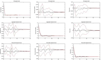
An advantage of TVP models is that it allows us to draw a whole picture of shocks along
with the time line and pick up a specific year to analyze. Also, it allows us to get a
ten-dency of change with each shocks (i.e. the increasing tenten-dency of the supply shock during
certain years). The shocks of oil supply, aggregate demand and oil-specific demand are
drawn in Figure 4.1. From the plot, the supply shock has the highest volatility during
Figure 4.1: Posterior mean, the standard deviation of residuals for shocks
Embargo happened and before Iranian revolution. Also this event shows a coincidence
with stagnation on the U.S. macroeconomy. After 1990, its volatility gradually decreases
and it reached a lower peak during the Iran-Iraq War and Gulf War. The supply shock
becomes less volatile during the Venezuela civil unrest and Iraq War period between the
three shocks, though little volatility shows up in 2003. This finding is consistent with
Kilian’s, which says there shows no evidence of a oil supply disruption in 1978-1980 but
a disruption associated with the Iran-Iraq War period.
The aggregate demand shock has same co-movement with the supply shock, but it has
smoother shape and smaller range than the supply shock. The co-movement gets the
same result of Kilian’s (2009), but Kilian’s historical decomposition of shocks did not
its different tendency from other two shocks. It has the almost opposite direction with the
supply shock: high volatility before Embargo and it decreased quickly to a very low level
during the Iranian revolution and at the beginning of the Iraq war. The high volatility
shows up after the Iraq war also at the OPEC collapse, and then during the Gulf War,
it reaches to its peak.
The plot also exhibited an opposite relationship between the supply and oil-specific
de-mand shocks. The supply shock has a higher volatility before 1990, while the oil-specific
demand shock goes the opposite direction to the supply shock. To be more explicit:
dur-ing the Embargo and Iranian revolution period, there was an impact to the oil supply.
Due to the impact, oil price went up and therefore caused the macroeconomy to fluctuate.
During the period of the Iran-Iraq War, the supply shock was persistent, but the demand
shock diminishes very quickly. The reason of the sudden increase in the demand shock
seems connected more with the OPEC collapse not the war due to the OPEC collapsed
that happened in 1985. After 1990, during and after the Gulf War period, the supply
and oil-specific demand shocks turned over. The supply shock stays stable in a lower
level while the oil-specific demand shock is gradually increasing. This confirms Hooker’s
(1996) view that the War shifted the demand side of oil not the supply side. Furthermore,
this finding could explain that after the War, the economy does not simply rely on the
oil from Middle east or South American, and a single area experiencing a disruption of
oil supply could not make a big impact to economy like the 1970s any longer. Another
interesting finding based on the opposite direction of supply and demand shocks is that
the plot finds a way to explain why early researchers focus on oil-supply side while later
researchers like Kilian asked to concentrate on the oil demand side to the impact of
macroeconomics. For more details of each event, the analyses are presented below and
in Appendix C.
i)the October War/Embargo period
From Figure C.1, the impact between the structural impulse response shocks before the
War and after the War is obvious. Both of the shocks in oil supply and oil-specific demand
to oil production and real price of oil have larger volatility compared to the economic
activity, while the aggregate demand shock does not possess this property. Also, the
oil-specific demand shock shows a different time-varying property on price of oil with other
two shocks: the oil-specific demand shock has one time time-varying effect while two
other shocks have longer lasting time-varying effects. This phenomenon can be confirmed
by checking Figure 4.1, that the oil-specific demand shock is not as dominant as supply
shocks before 1990. Furthermore, the structural impulse response of oil-specific demand
shock to oil production became even smaller after war ended, which means the demand
shock does not help much to interpret Embargo with a macroeconomic relationship
dur-ing the Embargo period. The third finddur-ing is that the plot of the difference of structural
impulse responses of each shock to the price of oil are persistent compared to the later
five periods, which suggests during the Embargo period, the price of oil has a bigger
impact on oil-price shocks.
ii) the Iranian revolution period
The plot of structural impulse responses are shown in Figure C.2. From the plots, the
responses are exploding during the Iranian revolution period. Furthermore, I check the
structural impulse responses during 1979 when the Iranian revolution ended to 1986
when one year after OPEC collapsed, the structural impulse responses are always
responses disappear (the plot is shown in Figure C.3). This finding may reject the suspect
that there exists unit root during this period. And Phelps (1994), Carruth et al. (1995)
and Hooker (1996) suggested real oil prices cannot actually contain a unit root. In the
end, the exploding structural impulse response is still left to be investigated further in
the future.
For the subplots of structural impulse responses’ difference, both of the three shocks to
the price of oil shows little time variance. But both of the shocks to oil production possess
a significant time varying effects. Among the effects, both the oil supply shock and
oil-specific demand shock have negative impact in the first period (month) while aggregate
demand shock have a positive impulse to oil production.
iii) the Iraq-Iran War period
The Iraq-Iran War lasted for 8 years, but I did not select to compare the structural
im-pulse responses across the 8 years due to the unstable structural imim-pulse responses stated
in the last part, what selected here is the structural impulse response at 1988 when the
war went to end compares to 1986 when the exploding structural response disappeared.
As Figure 4.1 shows that the Iraq-Iran war was in a transit period when supply shock and
aggregate demand shock stayed in a middle low position and oil-specific demand shock
gradually increased, the Figure C.4 plots structural impulse responses of two periods and
its differences. For the plot, the effect of the supply shock to economic activity decreases
and to oil production increases compared with previous periods. The decreases of supply
shock to economic activity should have more strength than the shock to oil production
due to the War that happened in the supply shock decreasing period. The supply shock
to the price of oil did not impact much during the War, and from the difference of the
than the Embargo period.
From Figure 4.1, the oil-specific demand shock does not show a big fluctuation during
the war period. And for the structural impulse response plot, the shock to oil production
and shock to economic activity cancelled each other, and the shock to price of oil does
not show any time-varying effect.
At last, during the Iraq-Iran war period, the supply shock and aggregate demand shock
pulls the oil production down while oil-specific demand shock pushes it up. But for the
shocks to economic activity, the supply shock and aggregate demand shock pushes it
down and oil-specific demand shock pulls it up. Both of the shocks show less time
vary-ing on the price of oil.
iv)the Gulf War period
The Gulf War happened in a transit period when the oil-specific demand shock becomes
strong while the supply shock decreases to the bottom. During this period, I compare
with the structural impulse responses when the year the Gulf War ended and two years
before the Gulf War ended (the plot is in Figure C.4), and I found that the oil supply
shock to real activity gets a higher fluctuation compares to the oil production and the
price of oil. Also for the plot of the difference of structural response between after the
war happened and before the war happened, there also exhibits high fluctuation in the
oil-specific demand shock to oil production and to the price of oil. Overall, the shocks
during the Gulf War period are similar to shocks during the Iraq-Iran War period, except
that the Gulf War period shows bigger range of shocks, and the shocks to the price of oil
show more time variation than the Iraq-Iran War period.
The plots of structural impulse responses of the Venezuela civil unrest and Iraq War
periods are shown in Figure C.5 and Figure C.6. Compare the oil-specific demand shock
of these two periods to the shock of the Embargo period, the shock to the oil production
and to real activity was increasing while the shock to the price of oil was decreasing. Since
from Figure 4.1 we know both of the two periods are in the demand shocks dominating
period, there suggests the increase of the oil-specific demand shock to oil production and
real activity overwhelmed the decreases of that to the price of oil.
The supply shock to oil production and economic activity are increasing between those
two periods when compared to the Embargo period, while the price of oil is decreasing.
Since the supply shock has been gradually decreasing after 1990, and the aftermath of
its decreasing compared to the price of oil has a dominant effect to pull down the supply
shock than the supply shock to the oil production and economic activity to push it up.
The aggregate demand shock to the oil production and economic activity have a stronger
impact than that of the Embargo period, while the shock to the price of oil are decreasing,
since the aggregate demand shock has the same tendency as the oil supply shock. The
decreasing of shock to price of oil is much stronger effect than it to the oil production
and activity.
Also, and interesting phenomenon exists between the period of Venezuela civil unrest and
the Iraq War in that they have an opposite relationship on the plots in their structural
impulse responses difference. For example, in the difference plot of oil supply shock to
oil production, there has a positive impact at first during the Venezuela civil war, while
there was a negative impact during the Iraq War.
To summarize all of the plots, for the shocks to the price of oil, the Embargo period
has the most time-varying effect and then the effect decreases in the following periods.
become more and more time-varying in later events. The time-varying effect of shocks to
Chapter 5
Model comparison and convergence
diagnosis
5.1
The conventional structural VAR model
The conventional structural VAR model applies the Kilian’s (2009) least-square model
with short-run restrictions. The lags are selected to 10, which is the minimal lag to
ex-hibit persistent impulse responses.1 The plot of its structural impulse responses is shown
in Figure 5.1 with bootstrap confidence interval. From the plot, the volatility of each
structural impulse response is almost appeased after 12 periods. The supply shock to
the price of oil and economic activity shows an opposite direction of impulses. Between
the three shocks, demand shocks have larger shocks both to the oil production, economic
activity and price of oil. This result is consistent with Kilian’s.
1The SIC criteria gives a lag of 2. Under lags with 2, all of the structural impulse responses return
Figure 5.1: Structural impulse response of the conventional structural VAR model
5.2
The time invariant parameter structural VAR
model and model comparison
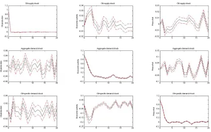
This part plots the structural impulse response function of the time-invariant-parameter
structural VAR model, where the model is shown in chapter 3.3 with selected lags to
10 according to the conventional structural VAR model. The plot of structural impulse
responses are shown in Figure 5.2.
From Figure 5.2, the structural impulse response performs similarly to the least-square
structural VAR model. For example, the demand shocks have a bigger range than the
supply shock to both of three factors. But some differences exist. Unlike the
conven-tional model, the time-invariant-parameter model gives a more wild structural impulse
conventional‘s, and so does the performance of oil-specific demand shock. Furthermore,
the structural impulse responses are more persistent in shocks in the
time-invariant-parameter model than the conventionals responses. For the oil supply shock to the price
of oil, the impulse responses at 15 periods become stronger than the previous periods.
This performance may suggest the structural impulse responses of time invariant
param-eter does not show any advantage on performing shock.
Figure 5.2: Structural impulse response of the time invariant VAR model
Next I would like to compare the structural impulse response of time-invariant model
with the TVP model. The TVP model has smaller range compared to time-invariant
model gives a smaller range of -0.005 to 0.004 compared to the time invariant parameter
model with -0.5 to 0.5. The structural impulse responses of the TVP model also has a
smaller range compared to the least-square VAR model, and the shocks perform more
flatly.
5.3
Sensitivity analysis
Also, choosing kQ = 0.01, kS = 0.1 and kW = 0.01 is almost a standard setting. In
this section I would like to check the model‘s sensitivity to the change of the value of
priors, that is to change the value of of kQ, kS and kW’s values. Here are the selected 18
combinations of kQ ={0.01; 0.05; 0.1},kS ={0.01; 0.1; 0.5} andkW ={0.001; 0.01}. The
result shows that both changing the value of kQ, kS and kW do not change plot of each
shock (Figure 4.1) much. This suggests the model is fitting well to reflect shocks. I also
found if kS is bigger than 0.5, it will cause a singular matrix in sampling BT.
5.4
Convergence diagnostics for hyperparameters and
volatilities
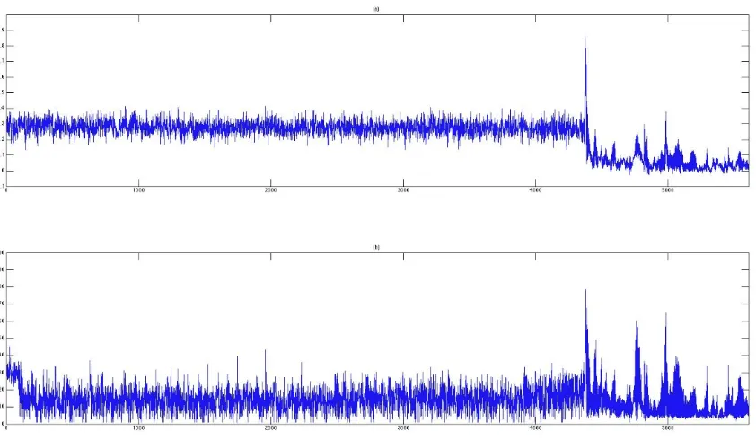
This part diagnoses the convergence of the Markov chain Monte Carlo algorithm in the
TVP model. There are total 5608 of hyperparameters and volatilities‘ convergence
diag-nose are made, with 4371 free parameters of Q, 4 free parameters ofS, 6 free parameters
of W and 1227 free parameters of Σ. The plots are shown in Figure 5.3 with 1-4371
Figure 5.3: Convergence diagnostics for hyperparameters and volatilites.
is the draws of the 20th order sample autocorrelation and (b) is draws of inefficiency
factors for the posterior estimates of the parameters. From (a), most of the parameters
have correlation around 0.3. Some of them are around 0.1, which suggests low correlation
between draws of each parameters, which suggests the draws are almost independent and
the chain mixed well. From plot (b), the IFs can be calculated by using Geweke’s (1992)
method withIF = (1+2PM
k=1ρk), whereM is approximated by using Newey and West’s
(1994) method, and ρk is thek-th autocorrelation of the chain. From the plot, most IFs
are below or around 20, except for a few IFs in Σ. This result suggests a low level of IFs.
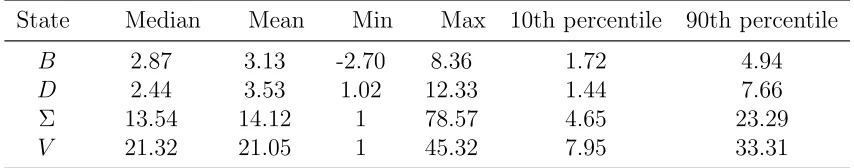
Furthermore, I summarize the statistics of IFs for each TVP parameter in Table 5.1.
From the table, the average IFs are around or below 20 which suggests an efficiency of
distributions of the parameters. V has the highest IFs, which are between 8 to 33.B has
Table 5.1: Summary of the distribution of the IFs for different sets of parameters.
State Median Mean Min Max 10th percentile 90th percentile
B 2.87 3.13 -2.70 8.36 1.72 4.94
D 2.44 3.53 1.02 12.33 1.44 7.66
Σ 13.54 14.12 1 78.57 4.65 23.29
V 21.32 21.05 1 45.32 7.95 33.31
of B are below−0.5, but the 10th percentile of B are positive and the negative numbers
outside the 10th percentile could be neglected. Also we could observe Σ has the largest
IFs at 79, but when checking, the 90th percentile is just 23, which suggests 79 is just an
Chapter 6
Conclusion
This paper extends Kilian’s research on oil shocks by using a TVP model and Markov
chain Monte Carlo methods. The plot of volatility states suggests there exists a gradually
decreasing tendency of the supply shock and aggregate demand shock, and a gradually
increasing tendency of the oil-specific demand shock. The transit period of the supply
and aggregate demand shock increasing and the oil-specific demand shock decreasing
happened in the year between 1980 and 1990 during the Iraq-Iran war. This finding could
explain why earlier researchers were inclined to analyze the supply shock, but Kilian’s
recent works found the oil-specific demand shock should be considered in investigating
oil-to-macroeconomy relationship. Besides the plot of volatility states, the analysis of the
structural impulse responses for 6 different selected events helps identify which factors
(oil production, economic activity and price of oil) impact which shocks the most. The
analysis of the Embargo period finds the oil supply and oil-specific shock to oil production
and the real price of oil have a bigger time varying impact than to the economic activity.
But during the Iraq War the time varying shock of oil supply shock to price of oil is less
there exists an unexplained exploding structural impulse responses during the Iranian
revolution period, but the unit root disappears for non-structural impulse responses.
This paper also compares with TVP, time-invariant-parameter and least-square models.
The advantages of the TVP model are that it could get structural impulse responses in
the specific year. Also, the TVP model possesses both a smaller range and nice shape
of structural impulse responses than the time-invariant-parameter model. For several
reasons, it should be considered the best model in interpreting shocks to economics
factors.
The last part did some diagnoses to the TVP model. One diagnosis is to check the
sensitivity of TVP models in respect to different priors. As a result, the changing of
different values ofkQ,kS, kW do not affect the results much, which suggests the model is
persistent to the results of analysis. Furthermore, it did the convergence diagnosis of each
REFERENCES
[1] Balke, N.S., Brown, S.P.A., Y¨ucel, M.K. 1999. Oil price shocks and the U.S. econ-omy: where does the asymmetry originate? Working paper, Federal Reserve Banks of Dallas.
[2] Barsky, R.B., Kilian, L. 2001. Do we really know that oil caused the great stagflation? A monetary alternative. NBER Macroeconomics Annual, 16(2001): 137-183.
[3] Barsky, R.B., Kilian, L. 2004. Oil and the Macroeconomics since the 1970s. The Journal of Economic Perspectives, 18(4): 115-134.
[4] Berkowitz, J., Kilian, L. 2000. Recent developments in bootstrapping time series.
Econometric Reviews, 19(1): 1-48.
[5] Bernanke, B.S., Gertler, M., Watson, M., Sims, C.A., Friedman, B.M. 1997. Sys-tematic monetary policy and the effects of oil price shocks. Brookings Papers on Economic Activity, 1: 91-157.
[6] Bollerslev, T. 1986. Generalized autoregressive conditional heteroskedasticity. Jour-nal of Econometrics, 31: 307-327.
[7] Burbidge, J., Harrison, A. 1984. Testing for the effects of oil-price rises using vector autoregression. International Economic Review, 25(2): 459-484.
[8] Carter, C.K., Kohn, R. 1994. On gibbs sampling for state space models.Biometrika, 81(3): 541-553.
[9] Cogley, T., Sargent, T.J. 2001. Evolving post world war II US inflation dynamics.
NBER Macroeconomics Annual, 16: 331-373.
[10] Cogley, T., Sargent, T.J. 2005. Drifts and volatilities: monetary policies and out-comes in the post WWII US. Review of Economic Dynamic, 8: 262-302.
[11] Daniel, B.C. 1997.Internatinal interdependence of national growth rates: a structural trends analysis. Journal of Monetary Economics, 40: 73-96.
[12] Dejong, D.N., Whiteman, C.H. 1993. Estimating moving average parameters: clas-sical pileups and bayesian posteriors. Journal of Business & Economic Statistics, 11(3): 311-17.
[14] Engle, R.F. 1982. Autoregressive conditional heteroscedasticity with estimates of the variance of United Kingdom inflation. Econometrica, 50(4): 987-1007.
[15] Ferderer, J.P. 1996. Oil price volatility and the macroeconomy: a solution to the asymmetry puzzle. Journal of Macroeconomics, 18: 1-16.
[16] Fern´andez-Villaverde, J., Rubio-Ram´ırez, J.F., Sargent, T.J., Watson, M.W. 2007.
ABCs (and Ds) of understanding VARs. The American Economic Review, 97(3): 1021-1026.
[17] Fr¨uhwirth-Schnatter, S. 1992. Data augmentation and dynamic linear models. Insti-tut f¨ur Statistik, 28.
[18] Ghent, A.C. 2009. Comparing DSGE-VAR forecasting models: How big are the differences? Journal of Economic Dynamics & Control, 33: 864-882.
[19] Gourieroux, A.M., Renault, E. 1993. Inditrect Inference. Journal of Applied Econo-metrics, 8: S85-S118.
[20] Hamilton, J.D. 1983. Oil and the Macroeconomy since World War II. Journal of Political Economy, 91(2): 228-248.
[21] Hamilton, J.D. 2003. What is an oil shock?Journal of Econometrics, 113: 363-398.
[22] Harvey A.C. 1990. Forecasting, structural time series models and the kalman filter.
Cambridge Universit Press.
[23] Hooker, M.A. 1996. What happened to the oil price-macroeconomy relationship?
Journal of Monetary Economics, 38: 195-213.
[24] Hooker, M.A. 1999. Oil and the Macroeconomy revisited. Federal Reserve Board, Stop 71. 20th & C St., NW. Wahsington, DC 20551 mhooker@frb. gov.
[25] Ingram, B.F., Whiteman, C.H. 1994. Supplanting the ’Minnesota’ prior forecast-ing macroeconomic time series usforecast-ing real business cycle model priors. Journal of Monetary Economics, 34: 497-510.
[26] Jo, S. 2012. The effects of oil price uncertainty on global real economic activityBank of Canada Working paper, 2012-40.
[27] Kilian, L. 2008a. A comparison of the effects of exogenous oil supply shocks on output and inflation in the G7 coutries. Journal of the European Economic Association, 6(1): 78-121.
[29] Kim, S., Shephard, N., Chib, S. 1998. Stochastic volatility: likelihood inference and comparison with ARCH models. The Review of Economic Studies, 65(3): 361-393.
[30] Lee, K., Ni, S., Ratti, R.A. 1995. Oil shocks and Macroeonomy: The role of price variability. Energy Journal, 16(4): 39-56.
[31] Litterman, R.B. 1986. Forecasting with Bayesian vector autoregressions: Five years of experience. Journal of Business & Economic Statistics, 4(1): 25-38.
[32] Mork, K.A. 1989. Oil and the Macroeconomy when prices go up and down: An extension of Hamilton‘s results. Journal of Political Economy, 97(3): 740-744.
[33] Mork, K.A., Olsen, ø., Mysen, H.J. 1994. Macroeconomics responses to oil price increases and decreases in seven OECD coutries. Energy Journal, 15: 19-35.
[34] Muellbauer, J., Nunziata, L. 2001. Credit, the stock market, and oil.Working paper, University of Oxford.
[35] Negro, M.D., Schorfheide, F. 2004. Priors from general equilibrium models for vars.
International Economic Review, 45(2): 643-673.
[36] Negro, M.D., Schorfheide, F. 2009. Monetary policy analysis with potentially mis-specified models. The American Economic Review. 99(4): 1415-1450.
[37] Negro, M.D., Primiceri, G.E. 2013. Time varying structural vector autoregressions and monetary policy: Appendix to the corrigendum. Unpublished version.
[38] Nelson, E. 1998. Sluggish inflation and optiming models of the business cycle.Journal of Monetary Economics, 42: 303-322.
[39] Ni, S., Sun, D. 2003. Noninformative priors and frequentist risks of Bayesian esti-mators of vector-autoregressive models. Journal of Econometrics, 115: 159-197.
[40] Primiceri, G.E. 2005. Time varying structural vector autoregressions and monetary policy. The Review of Economic Studies, 72(3): 821-852.
[41] Pindyck, R.S. 1980. Energy price increases and macroeconomic policy. Energy Jour-nal 1, 120.
[42] Ruge-Murcia, F. 2012. Estimating nonlinear DSGE models by the simulated method of moments: With an application to business cycle. Journal of Economic Dynamic & Control, 36: 914-938.
[44] Sims, C.A., Zha, T. 1998. Bayesian methods for dynamic multivariate models. In-ternational Economic Review, 39(4): 949-968.
[45] Sims, C.A., Zha, T. 1999. Error bands for impulse responses. Econometrica, 67(5): 1113-1155.
[46] Todd, R.M. 1984. Improving economic forecasting with Bayesian vector autoregres-sion. Federal Reserve Bank of Minneapolis Quartely Review, 8(4): 18-29.
Appendix A
Derive posteriors of
B
T
,
D
T
and
Σ
T
in the TVP model
Section 3.2 (ii) gives a framework of deriving the posterior of BT. In this section gives
more details of deriving the sampling of BT, DT and ΣT based on Carter and Kohn
(1994), Fr¨uhwirth-Schnatter (1994) and Primiceri (2005).
i. Sampling BT
To sampleBT, first to assume the mean and variance ofp(BT|yT, DT,ΣT, V) areBt|tand
Pt|t and of p(Bt|Bt+1, yT, DT,ΣT, V) are Bt|t+1 and Pt|t+1. Because
t νt
∼iid N( 0 0 ,
Rt 0
0 Q
)
Then given B0|0 and P0|0, the kalman-filter and backward recursion delivers:
Bt|t=Bt−1|t−1+Kt(yt−Xt0Bt−1|t−1),
Pt|t=Pt−1|t−1+Q+KtXt0(Pt−1|t−1+Q),
Bt+1 ∼N(Bt|t, Pt|t),
Bt|t+1 =Bt|t+Pt|tPt−+11|t(Bt+1−Bt|t),
Pt|t+1 =Pt|t+Pt|tPt−+11|tPt|t.
The draws of Bt|t,Pt|t, Bt|t+1 and Pt|t+1 are the draws from the posterior distribution of
BT.
ii. Sampling DT
For DT, the basic idea is the same as sampling BT, but there needs to reshape the
equation (3.5) first, to express as
Dtyˆt= Σtt and yˆt=yt−Xt0Bt
And DT can be written as a state-space model with
ˆ
yt=Ztdt+ Σtt
and
Zt =
0 0 · · · 0
−ˆy1,t 0 · · · 0
0 −ˆy[1,2],t · · · 0
..
. ... ...
0 0 · · · −ˆy[1,···,n−1],t
where ˆy[1,···,n−1],t = [ˆy1,t,· · · ,yˆn−1,t].
Then the posterior would be
p(DT|yT, BT,ΣT, V) =p(DT|yT, BT,ΣT, V)ΠTt=1p(Dt|Dt+1, yT, BT,ΣT, V)
and p(DT|yT, BT,ΣT, V)ΠTt=1 and p(Dt|Dt+1, yT, BT,ΣT, V) can be sampled by using
Kalman filter and backward recursion the same as sampling BT.
iii. Sampling ΣT
After BT and DT are sampled, the equation (3.5) can be transformed to
Dt(yt−Xt0Bt) = yt∗ = Σtt
In order to getlogσ, here the equation above must be set to a stochastic volatility model
yt∗∗= 2ht+et
ht=ht−1+ηt
where yi,t∗∗ = logyi,t∗ + 0.001, ei,t = log2i,t, hi,t = logσi,t. Also, et and ηt are
uncorre-lated. And the log2
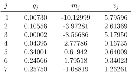
Table A.1: Selecion of the mixing distribution to belogχ2(1)
j qj mj vj
1 0.00730 -10.12999 5.79596 2 0.10556 -3.97281 2.61369 3 0.00002 -8.56686 5.17950
4 0.04395 2.77786 0.16735
5 0.34001 0.61942 0.64009
6 0.24566 1.79518 0.34023
7 0.25750 -1.08819 1.26261
Source: Kim, Shephard and Chib (1998)
a Bayesian way to approximate logχ2(1) to Gaussion distribution.
To sample the approximation of logχ2(1), donated by statesT, an selection of the mixing distribution table can be used. The table is shown in Table A.1.
Then the sampling algorithm is:
1. To use sampled DT and ΣT, a new value ofyt∗∗ can be obtained;
2. To obtain the probability mass function of state sT
P r(si,t =j|yi,t∗∗, hi,t)∝ {qj×normalpdf fN(yi,t∗∗|hi,t+mj−1.2704, vj2)},
Where i= 1,· · · , n;j = 1,· · · ,7;
3. To Initialize sT,h
t can be sampled with
p(ΣT|yT, BT, DT, sT, V) = p(ΣT|yT, BT, DT, sT, V)ΠTt=1p(Σt|Σt+1, yT, BT, DT, sT, V)
And p(ΣT|yT, BT, DT, sT, V),p(Σt|Σt+1, yT, BT, DT, sT, V) are the draws of ΣT sampled
Appendix B
Derive posteriors of
D
T
and
Σ
T
in
the time invariant parameter model
This appendix completes the posterior of DT and ΣT in time invariant parameter model
stated in section 3.3. I made the same transformation for DT and ΣT in Appendix A,
and the posterior of DT is:
P(D|yT, B,Σ)∼N( ¯d,D¯),
¯
D= (V ar( ˆD)/4 +Zt(ΣtΣ0t)
−1Z0
t)
−1,
¯
d= ¯D(V ar( ˆD))−1D/ˆ 4 +Zt(ΣtΣ0t)
−1yˆ
t
In a similar manner to derive posteriors of ΣT in the TVP model, we can transform the equation (5) to a state-space model of logσ. By initializing sT, the posterior of ΣT is:
¯
E = (V ar(logσˆ)−1/4 + 4St)−1,
logσ¯ = ¯E(V ar(logσˆ)−1/4 + 2Styt??)
Appendix C
Plots of structural impulse responses
in TVP model
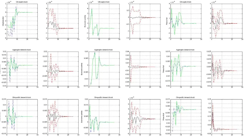
There are six events, each with 6 plots of structural impulse responses. The responses
plots the following periods: Embargo period, Iranian revolution period, Iraq-Iran War
period, Gulf War period, Venezuela civil War period and Iraq War period. Each plot has
18 subplots. The left plots are their structural impulse responses of shocks (supply,
ag-gregate demand and oil-specific demand) to economic factors (oil production, economic
activity and price of oil) of two selected years. To each of their right, the plot is the
difference of the two selected years’ structural impulse response and Bayesian 0.16 and
0.84 confidence intervals.
I selected each years of events as follows: 1) the Embargo period: 1973.2 and 1975.1; 2)
the Iranian revolution: 1977.12 and 1979.11; 3) the Iraq-Iran War: 1986.2 and 1988.1, ; 4)
the Gulf War: 1989.2 and 1991.1; 5) the Venezuela civil unrest: 2001.2 and 2003.1; 6) the
Iraq War: 2002.2 and 2004.1. All the dates are selected 1 year before events happened and
lasted 8 years, due to the exploding structural impulse response happened before 1986,
I did not select the year of 1980 when the war began. Also I plot the impulse response
of the Iranian revolution in the figure C.3. The impulse response shows there is no unit
roots exists during the period.
Plots of Structural impulse responses for each period:
Figure C.2: Structural impulse response during the Iranian revolution period
Figure C.4: Structural impulse response during the Iraq-Iran War period
Figure C.6: Structural impulse response during the Venezuela civil unrest period
Appendix D
Newey and West’s method of
obtaining
M
The M value in section 5.4 can be obtained by Newey and West (1994)’s algorithm.
The sample contains total 5608 parameters with each parameter has 8000 draws (the first
20% draws are treated as burn-in). For each parameter, say ˆht, where t = 1,2,· · · , T,
T = 8000, the algorithm is:
n= [4(T /100)2/9],
ˆ A= T X t=2 ˆ
hthˆ0t−1(
T
X
t=2
ˆ
ht−1hˆ0t−1)
−1
,
ˆ
ht
†
≡hˆt−Aˆˆht−1,
ˆ
σj = T
X
t=j+2
ˆ
h†tˆh†t−j, j = 0,1,· · · , n,
ˆ
s1 = 2
n
X
j=1
jσˆj,sˆ0 = ˆσ0+ 2
n
X
j=1
ˆ
ˆ
γ = 1.1447({s1/s0}2)1/3,
M = [ˆγT1/3].