Compositional Static Cache Analysis Using Module-level Abstraction

(1)

Patil, Kaustubh S.: Compositional static cache analysis using module-level abstraction (Under the direction of Dr. Frank Mueller).

Static cache analysis is utilized for timing analysis to derive worst-case execution time of a program. Such analysis is constrained by the requirement of an inter-procedural analysis for the entire program. But the complexity of cycle-level simulations for entire programs currently restricts the feasibility of static cache analysis to small programs. Com-putationally complex inter-procedural analysis is needed to determine caching effects, which depend on knowledge of data and instruction references. Static cache simulation tradition-ally relies on absolute address information of instruction and data elements.

(2)

by

Kaustubh S. Patil

A thesis submitted to the Graduate Faculty of North Carolina State University

in partial satisfaction of the requirements for the Degree of Master of Science in Computer Science

Department of Computer Science

Raleigh

2003

Approved By:

Dr. Alexander Dean Dr. Eric Rotenberg

(3)

Biography

Kaustubh S. Patil was born on 19th_{November 1979, in Mumbai, India. He received}

(4)

Acknowledgements

(5)

List of Figures

1.1 Framework used in static cache and static timing analysis . . . 1

2.1 Data-flow in the traditional integrated framework . . . 5

2.2 Data-flow in the new framework . . . 6

2.3 Module-level analysis ignoring calls . . . 7

2.4 Situation simulated by module-level analysis ignoring calls . . . 7

2.5 Module-level analysis considering calls . . . 8

2.6 Situation simulated by module-level analysis considering calls . . . 8

2.7 Module-level analysis with added outer-loops and ignoring calls . . . 9

2.8 Situation simulated by module-level analysis with added outer-loops and ig-noring calls . . . 9

2.9 Module-level analysis with added outer loops and considering calls . . . 10

2.10 Situation simulated by module-level analysis with added outer loops and considering calls . . . 10

2.11 Example of a module aligned on a cache-line size boundary . . . 11

2.12 Algorithm for bottom-up processing . . . 16

2.13 Example of the effect of two different paths in a module on the exit lines . . 17

2.14 Algorithm for obtaining final categorizations . . . 18

3.1 Compositional analysis example 1 . . . 35

4.1 Comparison of computation times for adpcmfor cache line size=16 bytes . . 39

4.2 Comparison of computation times for adpcmfor cache line size=32 bytes . . 40

4.3 Comparison of computation times for mmfor cache line size=16 bytes . . . . 41

4.4 Comparison of computation times for mmfor cache line size=32 bytes . . . . 42

4.5 Comparison of computation times for madfor cache line size=16 bytes . . . 43

4.6 Comparison of computation times for madfor cache line size=32 bytes . . . 44

4.7 Comparison of total compositional time with traditional time for adpcm, cache line size=16 bytes . . . 45

(8)

(9)

Chapter 1

Introduction

This chapter introduces the method of static cache analysis [18], which is used in static timing analysis to accurately predict the worst-case execution time for a program. In this method of static cache simulation for instruction caches, an instruction reference is categorized as a hit or a miss. It uses control-flow partitioning and a function instance graph for categorizing every instruction reference. The framework used for the static cache analysis and the static timing analysis is shown in Figure 1.1.

Source Files

Simulator Cache

Static _Cache

Categorization Analyzer

Timing WCET

Prediction Control Flow &

I/D−References Gcc (PISA)

Compiler

Figure 1.1: Framework used in static cache and static timing analysis

1.1 Static cache simulation

(10)

graph for the whole program is constructed. Then, this graph is analyzed to determine the program lines that can possibly be cached before entering each basic block of the program. In the last phase, this information is used to categorize each instruction reference.

1.1.1 Control-flow graph generation

Information about successors and predecessors of each basic block is generated using compiler back-end. Also, information about the function calls, if any, is collected for each basic block. Using this information, a control-flow graph is created for each function. Also, a function instance graph is generated for the whole program. An instance of a function refers to a unique invocation of that function. For example, if a function foo

can be reached from the function main using two different control-flows, then foo has two instances in the function instance graph.

1.1.2 Instruction reference classifications

An instruction reference is categorized based on the abstract cache state of the basic block that the instruction lies in. For each loop nesting and function nesting level, one category is derived for each instruction.

Potentially cached line: A program line can potentially be cached before entering a basic block if there exists a sequence of control-flow such that the line is cached when the basic block is entered along that control-flow.

Abstract cache state: An abstract cache state of a basic block in a function instance is the subset of all program lines that can potentially be cached before the execution of that basic block.

An instruction reference is categorized into one of these four categories.

• Always-Miss: An instruction is categorized as analways missif it cannot be guaran-teed to be in cache for that reference. Analways missis predicted when the instruction is the first reference to a program line in the basic block and the program line is not in the abstract cache state of that basic block.

(11)

abstract cache state, and no other conflicting program line is in the abstract cache state.

• First-Miss: An instruction is categorized as afirst missif it cannot be guaranteed to be in cache the first time it is accessed when the loop is entered, but it is guaranteed to be in cache for all later iterations of that loop.

• First-Hit: An instruction is categorized as afirst hitif it is guaranteed to be in cache the first time it is accessed when the loop is entered, but cannot be guaranteed for later iterations of that loop.

1.2 New compositional static cache analysis approach

This thesis proposes a method consisting of two stages to obtain categorizations for all instruction references in a program.

1.2.1 Module-level analysis

In module-level analysis, the control-flow information for only the module in ques-tion is used to obtain categorizaques-tions. The static cache simulaques-tion approach [18, 19] de-scribed in the previous section is used to perform module-level analysis. While doing module-level analysis, no absolute address information for instruction references is avail-able. Four different types of analyses are performed on each module. These are described in the next chapter. Module-level analysis is comparable to the creation of an object file during compilation process, in which only relative address information is available for each module.

1.2.2 Compositional analysis

(12)

1.3 Motivation

The static cache simulation approach described previously requires a time overhead comparable to that of data-flow analysis used in optimizing compilers, which can be quite high for large-sized programs involving complex control-flow patterns and nested structures. In the new approach, the burden of the time overhead is shifted to the module-level analysis, which needs to be done only once for each module, and it can be reused later for the complete analysis of any program that uses the module. Besides, the complexity of the second stage i.e. the compositional analysis, is lower than the traditional analysis of the entire program. Also the compositional approach predicts the categorizations without sacrificing any accuracy. The actual complexity estimations are explained in the next chapter.

In short, for the whole program, spacial locality cache effects are captured by cache simulation of module-intrinsic memory references during module-level analysis. During this first stage, the simulation of temporal locality is constrained to iterators within a module

i.e. only a subset of temporal reuse can be calculated during the module-level analysis. The second stage i.e. the compositional analysis captures the effects of temporal locality on categorizations across calls to modules.

1.4 Organization of the document

(13)

Chapter 2

Design of the Compositional

Approach Framework

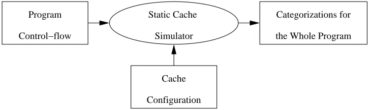
This chapter discusses the design of the new two-stage worst-case static cache analysis framework. Both the stages are described in detail. The new compositional ap-proach works for a fixed cache configuration. i.e. for both, the module-level analysis and the compositional analysis, the cache configuration remains the same. Currently worst-case analysis for direct-mapped instruction caches is supported in the implementation.

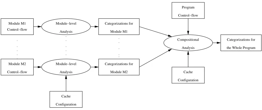
The data-flow that takes place during the traditional integrated approach is de-picted in Figure 2.1. This can be contrasted with the data-flow during the new approach which is shown in Figure 2.2.

Static Cache

Simulator Program

Control−flow

Categorizations for

the Whole Program

Cache

Configuration

(14)

Module M1 Control−flow Module M2 Control−flow Module−level Analysis Module−level Analysis Cache Configuration Module M1 Categorizations for Categorizations for Module M2 Program Control−flow Compositional Analysis Cache Configuration . . . . . Categorizations for the Whole Program . . . . . . . . . .

Figure 2.2: Data-flow in the new framework

2.1 Module-level Analysis

In the first stage, instructions are categorized only on the modular basis. During this stage, the module is considered to be laid out in its own address space starting with zero offset. The reason behind this requirement is explained in the next section. Also, at this level of analysis, no information is available about called modules, if any, except for the name of the modules. Four types of anlayses are performed on each module. These are described below. In all the examples of this section, the instruction cache is assumed to have four cache lines.

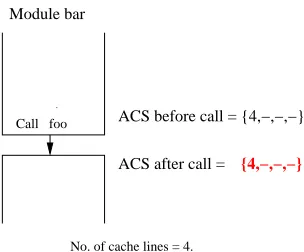
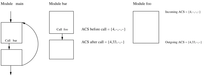
2.1.1 Module-level analysis ignoring calls

(15)

Call foo ACS before call = {4,−,−,−}

ACS after call = {4,−,−,−}

No. of cache lines = 4.

Module bar

Figure 2.3: Module-level analysis ignoring calls

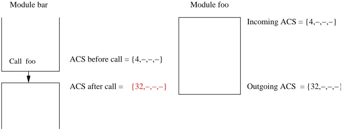
This analysis tries to capture the situation shown in Figure 2.4 that may occur during actual inter-procedural analysis.

Module bar Module foo

Incoming ACS = {4,−,−,−}

Outgoing ACS = {4,33,−,−} ACS after call = {4,33,−,−}

Figure 2.4: Situation simulated by module-level analysis ignoring calls

Every instruction reference for the module is categorized based on the ACS ob-tained using this assumption. Consider a program that uses this module. Consider a basic block B, such that its predecessor, P, has a call to a module. Consider a line l of the block P. If the called module does not cache in a line that maps to the same cache line as l, then for block B, the categorizations for an instruction of a line that maps to the same cache line as l will be exactly same as the one obtained for block B during the module-level analysis ignoring calls.

2.1.2 Module-level analysis considering calls

(16)

map to every cache line of the cache. i.e. the called module evicts all the cache lines in the ACS of the calling block and caches in its own lines.

Since the absolute address information for the lines of the called module is not known during module-level analysis, we indicate a line of the called module that conflicts with a line in the ACS of the calling block asC(a must-conflict line). Figure 2.5 illustrates the underlying assumption for the module-level analysis considering effect of the calls on the caller.

Call foo ACS before call = {4,−,−,−} ACS after call =

Module bar

{C,−,−,−}

Figure 2.5: Module-level analysis considering calls

This analysis simulates the situation shown in Figure 2.6 that might occur during the actual inter-procedural analysis.

Call foo

Module bar

ACS before call = {4,−,−,−}

Module foo

Outgoing ACS = {32,−,−,−} ACS after call = {32,−,−,−}

Figure 2.6: Situation simulated by module-level analysis considering calls

(17)

the ones obtained for block B during the module-level analysis ignoring calls.

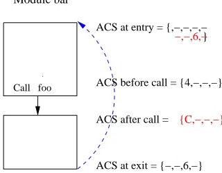
2.1.3 Module-level analysis with added outer loops and ignoring calls Before performing this analysis on a module, we add a back-edge from each exit block to each entry block of this module. These added outer loops simulate the return of the control-flow to this module during a program execution. Also, during ACS calculations, effects of the calls are ignored as in the first subsection. Figure 2.7 illustrates modification of a control-flow graph after addition of back-edges. Figure 2.8 shows the situation that is simulated by this analysis.

Call foo

Module bar

ACS after call = {4,−,−,−}

}

ACS at exit = {−,−,6,−} ACS at entry = {,−,−,−,−

−,−,6,−

Figure 2.7: Module-level analysis with added outer-loops and ignoring calls

Module main

Call bar

Module bar

ACS after call = {4,33,−,−}

Module foo

Outgoing ACS = {4,33,−,−}

Figure 2.8: Situation simulated by module-level analysis with added outer-loops and ignor-ing calls

(18)

module, and the control returns to this module from the calling loop for each loop iteration except for the first iteration.

The calls are ignored during this analysis. This simulates a call within this module that does not have any effect on the incoming ACS of the successor of the calling basic block.

2.1.4 Module-level analysis with added outer loops and considering calls As in the previous section, back-edges are added from exit blocks to entry blocks. But in this case, effects of the calls are considered. This simulates a module being called from a loop of another module, and the called module has a call that affects the incoming ACS of the successor of the calling block. Figure 2.9 illustrates the calculations during this analysis and Figure 2.10 shows the effects simulated by this analysis.

Call foo

Module bar

ACS after call = }

ACS at exit = {−,−,6,−} ACS at entry = {,−,−,−,−

−,−,6,−

{C,−,−,−}

Figure 2.9: Module-level analysis with added outer loops and considering calls

Module bar Module main

ACS after call = {32,−,−,−}

Module foo

Outgoing ACS = {32,−,−,−} Call bar

Call foo

Figure 2.10: Situation simulated by module-level analysis with added outer loops and con-sidering calls

(19)

loop-numbers to which the basic block belongs and for each loop, all the basic blocks that the loop contains are stored in files for that module.

2.2 Compositional analysis

Compositional analysis is performed on an entire program when the absolute ad-dress information for each module is available.

2.2.1 Need for module alignments

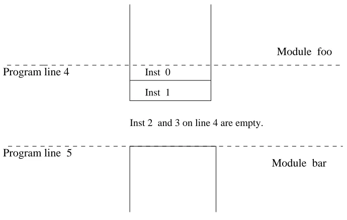
For the compositional analysis, it is assumed that a module is aligned on cache-line size boundary. I.e., a module can only start on the beginning of a new line and not within a line. This is not a necessary but rather a simplifying assumption to reduce the overhead involved in the module-level analysis. This is explained below in detail. Figure 2.11 illustrates this assumption.

Program line 4 Inst 0 Inst 1

Module foo

Module bar Program line 5

Module bar is aligned on cache line size = 4.

Inst 2 and 3 on line 4 are empty.

(20)

If this requirement were not enforced, then a module could start in many posi-tions w.r.t to a module above it in the process address space.The number of such possible combinations isO(number of instructions in a cache line).

Suppose a module is laid out in the address space in such a way that it starts on the third instruction of a program line. Now, we cannot use the module-level analysis performed in the first stage for this module. The reason for this lies in the changed interaction of basic blocks within the module in terms of the cached lines passed during data-flow analysis. So for such a ’non-aligned’ module, we need to use the module-level analysis, where we assume that the module starts on the third instruction of a program line. i.e. if we assume a four byte instruction, then the first instruction of this module will start from offset 8 during module-level analysis. If we do not enforce any restrictions on the starting offset of a module, we will need to perform the module-level analysis for each module O(number of instructions in a cache line) times. For a cache line size of 16 or 32 instructions, this imposes a significant overhead. Hence, the starting offset of a module is restricted to be a multiple of cache line size.

Besides, by imposing such an alignment for all modules, space wasted is at most O(1₂nf×cls) wherenfis the number of functions andclsis the cache line size. Most current architectures that use instruction caches have a cache line size of 32, 64 or 128 bytes. Hence, the space wasted will not be a significant overhead on the memory used during program execution.

2.2.2 Initial predicted categorizations

For each instruction of each module in the program, it is assumed that the module-level categorizations ignoring calls are the initial categorizations. These are optimistic cate-gorizations assuming that no temporal locality effects take place across module boundaries during control-flow transitions across calls. The compositional analysis is started with this assumption, and in the remaining processing, the necessary adjustments are applied to these categorizations.

Two kinds of adjustments are necessary for each line in each module.

(21)

Adjustments as a callee: When a module M is being called within a loop L of another module, then except the first iteration of L, the call to M within the remaining iterations might result in some lines of M still being present in the cache. Hence for those lines, we need to use the module-level analysis with added outer loops.

In the following subsection, the algorithm used is described and explained in detail.

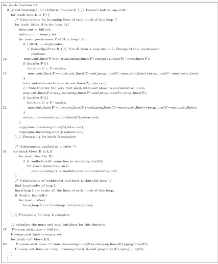
2.2.3 Bottom-up processing

In the compositional analysis stage, a limited amount of analysis is done in order to obtain the inter-procedural relationship in terms of the cached lines passed across the module boundaries during calls and call returns. The modules are processed starting from the leaf module in a call graph and gradually traversing the graph toward the rooti.e. the

main function. The algorithm for a basic block used in the bottom-up processing is given in Figure 2.12.

As can be seen, the bottom-up processing is done for each module only once. The complexity of the above algorithm is O(nf×nlf ×nbl×npb) where nf is the number of modules, nlf is the maximum number of loops in any one module, nbl is the maximum number of basic blocks in any one loop and npb is the maximum number of predecessors of a basic block. Thus, the complexity of this algorithm that captures the inter-procedural analysis information is kept at module-level. I.e., for a module, there is no need to reanalyze its callees, thus, saving time overhead.

Lines belonging to each loop are calculated. Also each loop is assigned its own loopheader. The must exit lines for a module (mentioned in line 47 of the algorithm) store the lines that are guaranteed to be in cache when the control of execution returns from the module. The may exit lines for a module are the lines of that module that may be present in the cache on exit from the module, but their presence in cache cannot be guaranteed. For instance, if a line l of a module lies on one path P, but not on some other path P’ of the module, and, following the control-flow along the path P, it is present in the outgoing lines of a specific exit block, then the line willnot be present in the must exit lines of the module as it might not be cached if the control-flow goes along P’. It will be present in the may exit lines. This is further explained in the example given in the Figure 2.13.

(22)

getbit, then for the successor S of block B, it is necessary to consider the fact that, when the control returns to S, line 43 ofgetbit might be in the cache, as we are considering the worst-case scenario. Hence, such a line is denoted by a notationMC (a May-Conflict line)

in the exit lines ofgetbit.

Bottom-up processing gathers for each basic block, and for each loop that the block belongs to, the lines that are guaranteed to be in cache before control of execution enters that basic block (referred to as must incoming lines in Figure 2.12 ) and also the lines that cannot be guaranteed to be in cache before entering the basic block (referred to as may incoming lines ). Line 15 of this algorithm shows the formula for calculating the

must out lines for a basic block, if the block has a call. All the lines in the must out lines

calculated on line 12 that are in conflict with any of the may exit lines of the callee are subtracted. Note that here the set may exit lines of the callee is used. This ensures that the set must out lines calculated is safe and accurate. Then all the lines in must exit lines

of the callee are added, because these lines are guaranteed to be in cache when the control returns from the callee. Formula on line 22 similarly calculates themay out lines.

(23)

2.2.4 Adjustments to the categorizations as a callee

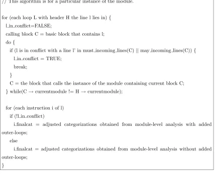
During this second and final pass of the compositional analysis, categorizations of each instruction might be adjusted depending upon whether the module is called by some other module or not. The algorithm for this pass is given in Figure 2.14. This algorithm is used for each linel in the program.

In the do while();loop of this algorithm we try to find out that, when the control returns to line l of the module from the call within loop L, if line l is still in cache. If it is, then it is going to be a hit, and we should use the categorizations from the simulated analysis with added outer loops.

2.3 Summary

(24)

for (each function F)

if (isleaf function||all children processed){// Ensures bottom-up order for (each loop L in F){

/* Calculations for incoming lines of each block of this loop */ for (each block B in the loop L){

inter out = full set; union out = empty set;

for (each predecessor P of B in loop L){

if ( B!=L→loopheader)

if (backedge(P-to-B)) // P-to-B form a loop inside L. Disregard this predecessor continue;

12: must out lines(P)=must incoming lines(P)-conf prog lines(P)+prog lines(P); if (iscaller(P)){

function C = P→callee;

15: must out lines(P)=must out lines(P)-conf prog lines(C→may exit lines)+prog lines(C→must exit lines);

}

inter out=intersection(must out lines(P),inter out);

// Note that for the very first pred, inter out above is calculated as union may out lines(P)=may incoming lines(P)-conf prog lines(P)+prog lines(P); if (iscaller(P)){

function C = P→callee;

22: may out lines(P)=may out lines(P)-conf prog lines(C→must exit lines)+prog lines(C→may exit lines);

}

union out=union(may out lines(P),union out);

}

copy(must incoming lines(B),inter out); copy(may incoming lines(B),union out);

}// Processing for block B complete

/* Adjustments applied as a caller */ 31: for (each block B in L){

for (each line l in B)

if (l conflicts with some line in incoming line(B)) for (each instruction in l)

normal category = module-level cat considering call;

}

/* Calculations of loopheader and lines within this loop */ find loopheader of loop L;

lines(loop L) = cache all the lines of each block of this loop; if (loop L has calls)

for (each callee)

lines(loop L) = lines(loop L)+lines(callee);

}// Processing for loop L complete

// calculate the must and may exit lines for this function. 47: F→must exit lines = full set;

F→may exit lines = empty set; for (each exit block E){

50: F→must exit lines =∩must incoming lines(E)-conf prog lines(E)+prog lines(E); F→may out lines =∪may incoming lines(E)-conf prog lines(E)+prog lines(E);

} }

(25)

Module getbit

Block 1

Block 2

Block 3

Block 4 Line 42

Line 43

Line 44

Line 45

Line 43 is cached along one path and not cached along other.

(26)

// This algorithm is for a particular instance of the module.

for (each loop L with header H the line l lies in){

l in conflict=FALSE;

calling block C = basic block that contains l;

do{

if (l is in conflict with a line l’ in must incoming lines(C)||may incoming lines(C)){

l in conflict = TRUE; break;

}

C = the block that calls the instance of the module containing current block C; }while(C→currentmodule != H→currentmodule);

for (each instruction i of l)

if (!l in conflict)

i.finalcat = adjusted categorizations obtained from module-level analysis with added

outer-loops;

else

i.finalcat = adjusted categorizations obtained from module-level analysis without added

outer-loops; }

(27)

Chapter 3

Examples Illustrating The

Compositional Analysis Framework

This chapter focuses on the description of three examples illustrating the various stages of the compositional approach introduced in the previous chapter. Source code for each example is given followed by the control-flow graph and the calculations for finding incoming lines and exit lines for each module. We start with explaining how the categoriza-tions derived from this framework are used to measure timing effects of instruction caches during timing analysis and follow up with the examples. By these examples, we explain the basic terms and notations used in this chapter.

3.1 Timing analysis

Excerpts of this section can be found in [6, 19]. The timing analyzer constructs a timing tree by traversing all paths within a loop level, and propagating this timing in-formation bottom-up within the tree. The timing tree represents the calling structure and the loop structure of the program. Functions are distinguished by their calling paths into function instances. Each function instance is regarded as a loop level with one iteration and is represented as a node in the timing tree. Regular loops are represented as child nodes of their surrounding function instance or as child nodes of another loop that they are nested in.

(28)

analyzed. When a child node, which represents a nested loop or invoked function, is en-countered along a path, its WCET is already calculated and can simply be added to the WCET of the current path after multiplying it with the number of iterations of the current nesting level. Adjustments are necessary for transitions from (1) first-misses to first-misses and (2) always-misses to first-hits between loop levels since the caching behavior of the instructions within these transitions is not the same for each invocation of the inner loop. Further comprehensive details of the timing analysis can be found in [6, 19].

3.2 Formulas for worst-case instruction categorizations

The definitions and formulas in this section are directly used from [19].

3.2.1 Definitions

• Linear Cache State (LCS) The linear cache state of a program line l within a basic block and a function instance is the set of program lines that can potentially be cached in the forward control-flow graph prior to the execution of l within the basic block and the function instance.

Informally, the LCS represents the hypothetical cache state in the absence of loops. This data-flow information represents the lines that may be cached between the entry of a loop to the current basic block on the first iteration. It will be used to determine whether a program line may be cached due to loops or due to the sequential control flow.

• Dominator Cache State (DCS) The dominator cache state of a program line l within a basic block and a function instance is the set of program lines that are known be cached prior to the execution of l within the basic block and the function instance.

The DCS can be used to determine if a program line must be cached due to an earlier reference, regardless of the sequence of execution paths that were taken.

• Post-dominator Set (PDS) The post-dominator set of a program line l within a basic block and a function instance is the self-reflexive transitive closure of post-dominating program lines.

(29)

3.2.2 Worst-Case Instruction Categorization

This subsection describes the formulas used in obtaining worst-case categoriza-tions. These formulas are based on the definitions given in the previous subsection.

• Letik be an instruction within a path, a loopλ, and a function instance.

• Letnbe the degree of associativity of the cache.

• Letl=i₀..im−1 be the program line containingikand letifirst be the first instruction

of lwithin the path.

• Let sj be the j-th component of the ACS (n-tuple) for l within the path and let

s= ∪

1≤j≤n

sj.

• Letl map into cache linec, denoted by l→c.

• Letu be the set of program lines in loopλ.

• Letchild(λ) be the child loop (inner-next loop within nesting) ofλfor this path and function instance, if such a child loop exists.

• Letheaders(λ) be the set of header paths andpreheaders(λ) be the set of preheader paths of loopλ, respectively.1

• Lets(p) be the abstract output cache state of path p.

• Letlinearj be the j-th component of the LCS (n-tuple) for l within the path and let

linear = ∪

1≤j≤n

linearj.

• Letdom be the set of dominating program lines (DCS) of path p.

• Letpostdom(p) be the set of self-reflexive post-dominating program lines of pathp.

(30)

                                                                

always-hit ifk6=first ∨(l∈dom∧

[∃

1≤j≤n

l∈sj∧( Σ

m→c,m6=l

|m∈sj|= 0∨ Σ

m→c,m6=l

|m∈s|< n)])

first-hit ifcategory(ik,child(λ)) =first-hit∨k=first ∧l∈s∧l∈dom∧

∀

p∈headers(λ)

l∈postdom(p)∧ Σ

m→c,m6=l

|m∈(s∩u)| ≥n∧

Σ

m→c,m6=l

p∈preheaders(λ)

|m∈((s(p)∪linear)∩u)|< n

first-miss ifcategory(ik,child(λ)) =first-miss∧k=first ∧l∈s∧

Σ

m→c,m6=l

|m∈s| ≥n∧ Σ

m→c,m6=l

|m∈(s∩u)|< n

always-miss otherwise

3.3 Example 1 of compositional analysis

int max(int,int); int a[10]; void main(){ int i; for(i=0;i<10;i++) a[i]=max(i,i); }

int max(int index,int i){

(31)

This program sets the array elements to the maximum of the indices or the initial value of the elements themselves. The control-flow graph for this program is shown in Figure 3.1.

3.3.1 Calculations in the traditional approach

The traditional calculations of abstract cache states are given below. In these calculations, line “I” indicates an invalid line. When the analysis begins, it is assumed that all the lines of the ACS are invalid lines. Also if an ACS is represented as [a b c d], this means program lineais mapped to cache line 0, line bis mapped to cache line 1 and so on. It should be noted that calculations for linear cache states (LCS), dominator cache states (DCS) and post-dominator sets (PDS) defined earlier are also performed in a similar way, but these calculations are not shown in these examples.

In all the examples the cache is assumed to contain four lines.

Pass 1:

in(1) = [I I I I] out(1) = [0 1 I I]

in(2) = [0 1 I I] out(2) = [0 1 2 I]

in(5) = [0 1 2 I] out(5) = [8 1 6 7]

in(6) = [8 1 6 7] out(6) = [8 9 10 7]

in(7) = [8 1 6 7] out(7) = [8 1 10 11]

in(8) = [8 9 10 7 out(8) = [8 9 10 11

1 11] 1 ]

in(3) = [8 9 10 11 out(3) = [4 5 2 3]

1 ]

in(4) = [0 1 I I out(4) = [0 I I

4 5 2 3] 4 5 2 3]

Pass 2:

in(1) = [I I I I] out(1) = [0 1 I I]

in(2) = [0 1 I I out(2) = [0 1 2 I

4 5 2 3] 4 3]

in(5) = [0 1 2 I out(5) = [8 1 6 7]

4 3]

(32)

in(7) = [8 1 6 7] out(7) = [8 1 10 11]

in(8) = [8 9 10 7 out(8) = [8 9 10 11

1 11] 1 ]

in(3) = [8 9 10 11 out(3) = [4 5 2 3]

1 ]

in(4) = [0 1 I I out(4) = [0 I I

4 5 2 3] 4 5 2 3]

The first column of categorizations in Figure 3.1 is based on these calculations. Our ultimate aim is to achieve the exact same categorizations using the new method.

3.3.2 Calculations in the new approach Step 1: Calculations ignoring all the calls

Here we assume that the calls make no change in the cache states of the basic blocks in the caller. Formain() and max(), we show the calculations below.

main():

Pass 1:

in(1) = [I I I I] out(1) = [0 1 I I]

in(2) = [0 1 I I] out(2) = [0 1 2 I]

in(3) = [0 1 2 I] out(3) = [4 5 2 3]

in(4) = [0 1 I I out(4) = [0 I I

4 5 2 3] 4 5 2 3]

Pass 2:

in(1) = [I I I I] out(1) = [0 1 I I]

in(2) = [0 1 I I out(2) = [0 1 I

4 5 2 3] 4 2 3]

in(3) = [0 1 I out(3) = [4 5 2 3]

4 2 3]

in(4) = [0 1 I I out(4) = [0 I I

4 5 2 3] 4 5 2 3]

(33)

in(5) = [I I I I] out(5) = [8 I 6 7]

in(6) = [8 I 6 7] out(6) = [8 9 10 7]

in(7) = [8 I 6 7] out(7) = [8 I 10 11]

in(8) = [8 9 10 7 out(8) = [8 9 10 11

I 11] I ]

We begin by assuming that the categorizations derived using these calculations (shown with “W/o calls” heading in Figure 3.1) are the initial categorizations and proceed by adjusting these to reflect the correct values.

Step 2: Adjustments for the caller

For the caller (main in this example) the possible differences in calculations may arise when the control returns to it after the callee is executed. Some cache lines in the cache state before the call might be evicted by the callee.

To handle this issue, first we need the ACS calculations for the caller with the assumption that after each call, the ACS is invalidated.

eg. for main():

Pass 1:

in(1) = [I I I I] out(1) = [0 1 I I]

in(2) = [0 1 I I] out(2) = [0 1 2 I]

// Return after the call

// Note the different connotations of I and C.

in(3) = [C C C C] out(3) = [4 5 2 3]

in(4) = [0 1 I I out(4) = [0 I I

4 5 2 3] 4 5 2 3]

Pass 2:

in(1) = [I I I I] out(1) = [0 1 I I]

in(2) = [0 1 I I out(2) = [0 1 I

4 5 2 3] 4 2 3]

// Return after the call

in(3) = [C C C C] out(3) = [4 5 2 3]

in(4) = [0 1 I I out(4) = [0 I I

(34)

Now, we focus on the exit lines of the callee (max). It should be noted here that though the line 9 is cached along one path it is not cached along the other. Hence, it does not appear in the exit lines but instead a line denoted by MC (as described in the previous chapter) is present in the exit lines. In this example, these are

out(8) = [8 MC 10 11]

This shows that the lines in the caller (main), which conflict with lines 8, MC, 10 and 11 of the callee, will certainly be evicted by the callee. We consider those lines in

main after the call site, which are in conflict with lines 8, MC, 10 and 11 of the callee, and for these lines we use the categorizations based on the calculations above as the final categorizations.

In general, we consider the conflicting lines between two call sites and adjust the categorizations. This approach completely adjusts the categorizations of the function as a caller.

Step 3: Adjustments for the callee

We need to calculate the ACS with the assumption that there is a back-edge from each exit block to the entry block of the callee function. In this example, these are not shown, but it is easy to see that all the instructions will be categorized as hits.

The call to max() in block 2 lies inside the loop of blocks 2 and 3. Now, we perform the ACS calculations only for this loop assuming an invalid ACS in the beginning of the header block (in this case, block 2) and ignoring the call. This yields

Pass 1:

in(2) = [I I I I] out(2) = [I 1 2 I]

in(3) = [I 1 2 I] out(3) = [4 5 2 3]

Pass 2:

in(2) = [4 5 2 3] out(2) = [4 1 2 3]

(35)

This shows that just before the second call to max, no line of maxwill be present in the ACS, as there is no [I] in the output ACS of block 3. Hence, the back-edge analysis need not be used for the callee and the analysis assuming invalid ACS in the beginning for the callee should suffice. On the other hand, if there was an [I] in the output ACS of block 3, we must use the back-edge analysis for that particular line in the callee, which conflicts with this [I]. This covers the adjustments required for the callee function.

3.4 Example 2 of compositional analysis

In this example we have a call graph of height 2. The code is as follows:

#include<stdio.h>

int a[10];

int rand(int);

int pseudo_rand(int);

int main(){

int i;

for(i=0;i<10;i++)

a[i]=rand(i);

return 0;

}

int rand(int i){

int val;

if((val=pseudo_rand(i)) > 50)

return val;

else

return 100-val;

}

int pseudo_rand(int i){

return 7*i+7;

(36)

The control-flow graph is depicted in Figure 3.2. The figure also lists the catego-rizations based on calculations with different assumptions.

Here most of the explanation for deriving the final categorizations remains the same, so we focus on the cache state calculations to check the validity of the approach.

3.4.1 Calculations in the traditional approach The traditional ACS calculations are given below:

Pass 1:

in(1) = [I I I I] out(1) = [0 1 I I]

in(2) = [0 1 I I] out(2) = [0 1 I I]

in(5) = [0 1 I I] out(5) = [0 1 6 I]

in(9) = [0 1 6 I] out(9) = [12 1 6 11]

in(6) = [12 1 6 11] out(6) = [8 1 6 7]

in(7) = [8 1 6 7] out(7) = [8 1 6 7]

in(8) = [8 1 6 7] out(8) = [8 9 10 7]

in(3) = [8 9 10 7] out(3) = [4 5 2 3]

in(4) = [0 1 I I out(4) = [0 I I

4 5 2 3] 4 5 2 3]

Pass 2:

in(1) = [I I I I] out(1) = [0 1 I I]

in(2) = [0 1 I I out(2) = [0 1 I I

4 5 2 3] 4 2 3]

in(5) = [0 1 I I out(5) = [0 1 6 I

4 2 3] 4 3]

in(9) = [0 1 6 I out(9) = [12 1 6 11]

4 3]

in(6) = [12 1 6 11] out(6) = [8 1 6 7]

(37)

in(8) = [8 1 6 7] out(8) = [8 9 10 7]

in(3) = [8 9 10 7] out(3) = [4 5 2 3]

in(4) = [0 1 I I out(4) = [0 I I

4 5 2 3] 4 5 2 3]

For the mainfunction, the ACS calculations assuming 1) no calls and 2) with calls and ACS invalidated on return are as follows:

Pass 1:

in(1) = [I I I I] out(1) = [0 1 I I]

in(2) = [0 1 I I] out(2) = [0 1 I I]

in(3) = [0 1 I I] out(3) = [4 5 2 3]

in(4) = [0 1 I I out(4) = [0 I I

4 5 2 3] 4 5 2 3]

Pass 2:

in(1) = [I I I I] out(1) = [0 1 I I]

in(2) = [0 1 I I out(2) = [0 1 I I

4 5 2 3] 4 2 3]

in(3) = [0 1 I I out(3) = [4 5 2 3]

4 2 3]

in(4) = [0 1 I I out(4) = [0 I I

4 5 2 3] 4 5 2 3]

Calculations considering calls and invalid ACS on return

Pass 1:

(38)

in(2) = [0 1 I I] out(2) = [0 1 I I]

in(3) = [C C C C] out(3) = [4 5 2 3]

in(4) = [0 1 I I out(4) = [0 I I

4 5 2 3] 4 5 2 3]

Pass 2:

in(1) = [I I I I] out(1) = [0 1 I I]

in(2) = [0 1 I I out(2) = [0 1 I I

4 5 2 3] 4 2 3]

in(3) = [C C C C] out(3) = [4 5 2 3]

in(4) = [0 1 I I out(4) = [0 I I

4 5 2 3] 4 5 2 3]

For the function rand( ), the calculations are as below:

Calculations assuming no calls

in(5) = [I I I I] out(5) = [I I 6 I]

in(6) = [I I 6 I] out(6) = [8 I 6 7]

in(7) = [8 I 6 7] out(7) = [8 I 6 7]

in(8) = [8 I 6 7] out(8) = [8 9 10 7]

in(5) = [I I I I] out(5) = [I I 6 I]

in(6) = [C C C C] out(6) = [8 C C 7]

in(7) = [8 C C 7] out(7) = [8 C C 7]

in(8) = [8 C C 7] out(8) = [8 9 10 7]

Finally for pseudorandom( ):

in(9) = [I I I I] out(9) = [12 I I 11]

(39)

3.5 Example 3 of compositional analysis

This small example has a conditional call. The code is as follows:

#include<stdio.h>

int a[] = {1,2,3,4,5,6,7,8,9,10};

int value (int i)

{

return a[i];

}

int main()

{

int sum = 0, i;

for(i=0; i<10; i++)

if(i)

sum += value(i);

return sum;

}

The control-flow graph is depicted in Figure 3.3. The figure also lists the catego-rizations based on different calculations.

As in the previous section, we focus on the cache state calculations to check the validity of the approach.

3.5.1 Calculations in the traditional approach The traditional ACS calculations are given below:

Pass 1:

in(2) = [I I I I] out(2) = [I I 2 3]

(40)

in(6) = [4 I 2 3] out(6) = [4 I 6 7]

in(1) = [4 I 6 7] out(1) = [0 1 6 7]

in(7) = [0 1 6 7] out(7) = [0 1 6 7]

in(4) = [4 I 2 3 out(4) = [4 I 2 3

0 1 6 7] 1 6 7]

in(5) = [4 I 2 3 out(5) = [4 5 6 3

1 6 7] 7]

Pass 2:

in(2) = [I I I I] out(2) = [I I 2 3]

in(3) = [I I 2 3 out(3) = [4 I 2 3

4 1 6 7] 1 6 ]

in(6) = [4 I 2 3 out(6) = [4 I 6 7

1 6 ] 1 ]

in(1) = [4 I 6 7 out(1) = [0 1 6 7]

1 ]

in(7) = [0 1 6 7] out(7) = [0 1 6 7]

in(4) = [4 I 2 3 out(4) = [4 I 2 3

0 1 6 7] 1 6 7]

in(5) = [4 I 2 3 out(5) = [4 5 6 3

1 6 7] 7]

For the mainfunction, the ACS calculations assuming 1) no calls and 2) with calls and ACS invalidated on return are as follows:

Pass 1:

in(2) = [I I I I] out(2) = [I I 2 3]

in(3) = [I I 2 3] out(3) = [4 I 2 3]

in(6) = [4 I 2 3] out(6) = [4 I 6 7]

in(7) = [4 I 6 7] out(7) = [4 I 6 7]

(41)

6 7] 6 7]

in(5) = [4 I 2 3 out(5) = [4 5 6 3

6 7] 7]

Pass 2:

in(2) = [I I I I] out(2) = [I I 2 3]

in(3) = [I I 2 3 out(3) = [4 I 2 3

4 6 7] 6 ]

in(6) = [4 I 2 3 out(6) = [4 I 6 7]

6 ]

in(7) = [4 I 6 7] out(7) = [4 I 6 7]

in(4) = [4 I 2 3 out(4) = [4 I 2 3

6 7] 6 7]

in(5) = [4 I 2 3 out(5) = [4 5 6 3

6 7] 7]

Pass 1:

in(2) = [I I I I] out(2) = [I I 2 3]

in(3) = [I I 2 3] out(3) = [4 I 2 3]

in(6) = [4 I 2 3] out(6) = [C C C C]

in(7) = [C C C C] out(7) = [C C C 7]

in(4) = [4 I 2 3 out(4) = [4 I 2 3

C C C 7] C 7]

in(5) = [4 I 2 3 out(5) = [4 5 6 3

C 7] 7]

Pass 2:

in(2) = [I I I I] out(2) = [I I 2 3]

in(3) = [I I 2 3 out(3) = [4 I 2 3

(42)

in(6) = [4 I 2 3 out(6) = [C C C C]

C ]

in(7) = [C C C C] out(7) = [C C C 7]

in(4) = [4 I 2 3 out(4) = [4 I 2 3

C C C 7] C 7]

in(5) = [4 I 2 3 out(5) = [4 5 6 3

C 7] 7]

For the function value( ), the calculations are as below. Calculations assuming no calls and calculations considering calls and invalid ACS on return are the same.

in(1) = [I I I I] out(1) = [0 1 I I]

(43)

restore

Block 4 jmp %i7+8

h h h

m m h

st

ld

nop

Block 5 save %sp, −104, %sp

%i1, [%fp+72] st %i0, [%fp+68] mov %i0, %o0

ble

sll %o0, 2, %o1 sethi %hi(a), %o0 or %o0, %l0(a), %o0

[%o1+%o0], %o1

mov %i1, %o0 cmp %o1, %o0

.L101 m h h h m h h h m h h h m h h h m h h h m h h h save %sp,−104,%sp Block 1

max( ) main( )

nop bge st %g0, [%fp−8] ld [%fp−8], %l0 cmp %l0, 10

.L95 m h h h m h m h h h m h m h h h m h Line 0 Line 1

Traditional W/o calls W/ calls

Line 2 Line 3 Line 4 Line 5 Line 6 Line 7 Line 8 Line 9 Line 10 Line 11 ld ld st Block 2 Block 3 [%fp−8], %o0

call max ld [%fp−8], %o1

mov %o0, %l2 [%fp−8],%l0 sll %l0, 2, %l0 sethi %hi(a), %l1 or %l1, %l0(a), %l1 st %l2, [%l0+%l1] ld [%fp−8], %l0 add %l0, 1, %l0

%l0, [%fp−8] ld [%fp−8], %l0 cmp %l0, 10

nop bl .L93

fh h fm m h h m h h h m h h h m h fh h fm h h h fm h h h fm h h h m h fh h fm m h h m h h h m h h h m h sethi st st restore Block 6 Block 7 Block 8 mov %i0, %o0

sll %o0, 2, %o1

%hi(a), %o0

or %o0, %lo(a), %o0

ld [%o1+%o0], %o0 ba .L103

%o0, [%fp−8]

mov %i1, %o0

%o0, [%fp−8]

ld [%fp−8], %i0 jmp %i7+8

m h h h m h h m m m h h m h h h m h h m m m h h

(44)

Block 1

nop

Block 2 call rand

Block 3

nop

Block 4

restore save %sp, −104, %sp st %g0, [%fp−8] ld [%fp−8], %l0 cmp %l0, 10 bge .L96

ld [%fp−8], %o0

mov %o0, %l2 ld [%fp−8], %l0 sll %l0, 2, %l0 sethi %hi(a), %l1 or %l1, %lo(a), %l1 st %l2, [%l0+%l1] ld [%fp−8], %l0 add %l0, 1, %l0 st %l0, [%fp−8] ld [%fp−8], %l0 cmp %l0, 10 bl .L94

mov %g0, %i0 jmp %i7+8

Block 5 save %sp, −104, %sp st %i0, [%fp+68] call pseudo_rand mov %i0, %o0

Block 6 st %o0, [%fp−8] ld [%fp−8], %l0 cmp %l0, 50 ble .L102 nop

Block 7 ld [%fp−8], %i0 jmp %i7+8 restore

Block 8 ld [%fp−8], %l0 neg %l0, %l0 add %l0, 100, %i0 jmp %i7+8 restore

Block 9 save %sp, −104, %sp st %i0, [%fp+68] mov %i0, %o0 sll %o0, 3, %o1 sub %o1, %o0, %o0 add %o0, 7, %i0 jmp %i7+8 restore main( )

rand( )

pseuod_rand( )

W/o calls W/ calls

m h h h m h fh h m h h h m h h h m h h h m m h h m h h h m h fh h fm h h h fm h h h fm h h h m m h h m h h h m h fh h m h h h m h h h m h h h m m h h m h h h m h h h h h m h m h h h m m h h h m h h h m h h h m h h h m h h h m h h h m m h h h m h h h m h h h m h h h m h h h m h h h m h h h m h h h m Line 0 Line 1 Line 2 Line 3 Line 4 Line 5 Line 6 Line 7 Line 8 Line 9 Line 10 Line 11 Line 12 Traditional

(45)

pushl %ebp

movl %esp, %ebp

movl 8(%ebp), %eax

movl a(,%eax,4), %eax

leave

ret

pushl %ebp

movl %esp, %ebp

pushl %esi

pushl %ebx

andl $−16, %esp

xorl %esi, %esi

xorl %ebx, %ebx

testl %ebx, %ebx

jne .L11

incl %ebx

cmpl $9, %ebx

jle .L8

popl %ebx

movl %esi, %eax

popl %esi

leave

ret

subl $12, %esp

pushl %ebx

call value

addl %eax, %esi

addl $16, %esp

jmp .L5 value() main() Line 0 Line 1 Line 2 Line 3 Line 4 Line 5 Line 6 Line 7 Block 1 Block 2 Block 3 Block 4

leal −8 (%ebp,%esp)

Block 6 Block 7 m h h h fm, m h m h h h m h h m fm, m m h h m h h h m h fm, m h m h h h

Traditional W/o call With call

m h h h m h m h h h m h m h h h m h h m fm, m h h h m h h h m h fm, m h m h h h m h h h m h h m fm, m m h h m h h h m h m h m m h h Block 5

(46)

Chapter 4

Experimental validation

This chapter describes the experiments performed to measure the performance improvement of the new compositional approach over the traditional approach and the accuracy of categorizations predicted by the new approach. Five benchmarks from the C-labs real-time benchmark suite [1] adpcm, ndes, cnt, mm and fft and one benchmark

(multimedia audio decoder - mad) from MiBench [2] embedded benchmark suite were

used.

4.1 Performance improvement

Time to perform static cache analysis using the traditional integrated approach and using the compositional approach were measured and compared for the six benchmarks for various cache configurations. Different cache configurations were used with the number of cache lines varying from 4 to 1024 lines (powers of 2) and size of each cache line varying from 8 bytes to 64 bytes.

(47)

com-parison purposes. This is in line with the main purpose of this thesis, which is to transfer the computational burden from the compositional stage to the module-level stage.

Figure 4.1: Comparison of computation times for adpcmfor cache line size=16 bytes

For adpcm the compositional approach takes lesser time than the traditional

ap-proach for all the cache configurations. The figures for adpcm also indicate that the com-positional approach scales better than the traditional approach. For instance, in Figure 4.1 the increase in traditional time for a change from 256 to 512 lines is about twice, whereas the increase for the compositional time is only about 1.5 times. Both Figures 4.1 and 4.2 show similar trend in the required computation time for the two approaches.

(48)

Figure 4.2: Comparison of computation times for adpcmfor cache line size=32 bytes

not provide enough opportunity for the compositional approach to exploit any complexity in the program structure, but as the number of cache lines increases, the overhead in the traditional approach increases with higher rate and hence the new approach produces better results.

madis a fairly large benchmark with around 9000 instructions. It consists of around 74 functions and the program structure involves complex loop and control-flow constructs. As is expected, there is a significantly large improvement in the compositional approach. For instance, the traditional approach takes about 1 hour for 512 lines compared to only about 32 seconds for the new approach. It should also be noted that for a cache line size of 16 bytes, more time is required than for 32 bytes cache lines.

(49)

Figure 4.3: Comparison of computation times for mmfor cache line size=16 bytes

calculating the compositional time.

Figure 4.7 shows that foradpcmthe total time for the two-stage approach is lesser than that for the traditional approach for cache lines ranging from 4 to 512. For a cache with 1024 lines, the time for the modular stage exceeds the traditional time and this causes the total time to be larger for the new approach. The modular stage performs 4 different analyses on each module, hence, this overhead increases with the increase in cache size. This explains the behavior for a cache with 1024 lines.

For mm (Figure 4.8), the total time for the new approach is greater than the tra-ditional time for all cache configurations. The reason for this remains the same i.e. the smaller size ofmm.

(50)

Figure 4.4: Comparison of computation times for mmfor cache line size=32 bytes

around 350 seconds compared to the 6600 seconds of the traditional approach. Thus results for fairly larger benchmarks (adpcm and mad) show that the compositional approach, even when applied just once for all the modules in a program, performs much better than the traditional approach. This is significant because it indicates that for such large programs, the new approach can result in large savings in computation time.

4.2 Accuracy of predicted categorizations

4.2.1 Comparison of worst-case execution cycles

(51)

Figure 4.5: Comparison of computation times for mad for cache line size=16 bytes

the new approach. Then the WCEC obtained using the two approaches were compared. The timing analyzer was run to perform analysis for Pseudo-Instruction Set Architecture

(PISA) [3]. To obtain the control-flow analysis information, the benchmarks were compiled using gccfor PISA (pgcc).

For all benchmarks exceptadpcm, for all cache configurations ranging from 4 cache lines to 512 cache lines, the WCEC were exactly the same. Foradpcmand ndes, the result of the timing analysis are summarized in tables 4.1 and 4.2 respectively.

For adpcm, results for a cache size of 64 lines show a tighter WCEC prediction

by the new approach. This is the only difference observed between WCEC for the two approaches. In this case, the traditional approach seems to categorize one instruction of

adpcm pessimistically from a first-miss to a miss. The new approach predicts categories

(52)

Figure 4.6: Comparison of computation times for mad for cache line size=32 bytes

using compositional approach. It is also interesting to note that as adpcmoccupies around 230 program lines in memory, it entirely fits in caches with 256 and 512 lines. I.e., once a program line is brought in cache, it will not be evicted later. Hence the WCEC for these two cache sizes are the same for this benchmark.

For ndes, as can be seen from the table, the estimated WCECs are exactly the same for the two approaches.

4.2.2 Comparison of WCEC with Simplescalar simulator

(53)

Figure 4.7: Comparison of total compositional time with traditional time for adpcm, cache line size=16 bytes

Number of cache Traditional Compositional %

lines WCEC WCEC change

512 9,227,240 9,227,240 0 256 9,227,240 9,227,240 0 128 18,590,441 18,590,441 0

64 23,751,141 23,651,041 -0.42

Table 4.1: Results of timing analysis ofadpcm

Table 4.3 shows the WCEC comparison for a direct-mapped cache with 64 lines and a line size of 16 bytes. For other cache configurations, similar results are observed. The WCEC ofmad could not be obtained due to constraints of path analysis within the timing analysis tool, a tool that is beyond the scope of this thesis.

4.3 Summary

The validity of the new approach is dependent on two metrics :

(54)

Figure 4.8: Comparison of total compositional time with traditional time formm, cache line size=16 bytes

Number of cache Traditional Compositional %

lines WCEC WCEC change

512 131,514 131,514 0

64 146,583 146,583 0

16 347,523 347,523 0

8 839,551 839,551 0

Table 4.2: Results of timing analysis of ndes

• the accuracy of the predicted categorizations.

(55)

Figure 4.9: Comparison of total compositional time with traditional time for mad, cache line size=16 bytes

Benchmark Predicted WCEC Observed WCEC Ratio

adpcm 23,740,141 17,549,967 1.35

ndes 146,298 95,147 1.54

fft 381,091 369,671 1.03

cnt 72,240 71,411 1.01

mm 2,037,588 2,034,313 1.01

(56)

Chapter 5

Future Work

The basic compositional static cache prediction approach can be extended to in-corporate more functionality. This is described in the following sections.

5.1 Support for set-associative caches

Currently, the compositional framework only supports direct-mapped instruction caches. The basic paradigm of this approach can be used for set-associative caches with some changes in the rules for adjusting the categorizations when a module acts as a callee and as a caller. For example, the incoming line calculations will change accordingly as each set can now have more than one cached lines. Also, the exit lines calculations for each module will change, and they need to be calculated for each set in the cache.

5.2 Best-case categorizations

(57)

5.3 Multi-level modular analysis

(58)

Chapter 6

Related Work

This chapter describes prior work on cache analysis and timing analysis. First, the general concepts related to static cache simulation approaches and the existing frame-works that use these concepts are introduced. This is followed by a summary of the new compositional analysis framework.

6.1 Prior methods

The main purpose of the various static cache simulation methods is their use in obtaining worst-case execution time (WCET) for a program. Bounding WCET estimations is important as schedulability analysis for hard real-time systems requires that the WCET be known in order to ensure feasibility of scheduling a task set for a given scheduling policy, such as rate-monotone and earliest-deadline-first scheduling [17].

Many different approaches have been used to obtain the WCET for a program. The combined use of the static cache analysis (Arnold et al. [4]) and the static timing analysis (Healy et al. [6]) provide fairly accurate WCET bounds. Our approach splits the static cache analysis into two stages, reusing the results from the first (module-level analysis) stage in the second (compositional analysis) stage, thus addressing the issue of computation overhead of cache analysis.

(59)

on simple CISC processors.

Zhang et al. [15] introduce an analyzable pipeline model that considers the effect of pipelined execution on timing analysis. The combined framework of [4] and [6] described above take instruction cache effects into account. These ideas and WCET analysis frame-work in [10] introduce timing analysis for pipelined RISC processors.

Liet al. [8] propose the use of Integer Linear Programming (ILP) formulation for capturing structural,functionality and cache constraints and solve them to obtain WCET. The ILP approach is extended to take cache timing effects into account. Rawat [16], Kim

et al. [7], Li et al. [9] and White et al. [14] extend the conventional static timing analysis to incorporate data cache timing effects.

Some instruction-level dynamic timing analysis methods assume the knowledge of an input set that would trigger the worst-case path during the actual program execution. Finding such an input set can be a non-trivial problem involving very high computational complexity. Even if such an input set is found, the actual execution-time effects of archi-tectural features onto timing analysis might cause a different input set to produce WCET. The integrated path and timing analysis method in Lundqvist et al. [11] combines dynamic cache analysis and dynamic timing analysis using instruction-level cycle-accurate simulation technique. The cache state at various points in the timing analysis is calcu-lated on the basis of the actual memory references made. The worst-case state is obtained by analyzing the cache state that will trigger worst-case response time in the remaining execution sequence. Thus, the cache calculations are integrated in the instruction-level simulation. Such approaches would suffer a significant computational overhead involved in cache calculations for fairly large programs that consist of a large number of possible execution paths.

Vera et al. [13] describe a technique of data cache locking to achieve predictable worst-case execution time for a program even when the execution environment has data caches. Unpredictability in WCET estimations is eliminated by locking those regions in the code that cannot be analyzed statically. Performance degradation possible due to cache locking is reduced by loading the cache with data likely to be accessed, but some overhead prevails.

(60)

from these as it focuses on the computation overhead involved in static cache analysis (performed separately from timing analysis), while preserving the accuracy of the predicted categorizations.

(61)

Chapter 7

Summary

This thesis contributes an approach to reduce the computation overhead involved in obtaining cache hit/miss information from static cache simulation for direct-mapped instruction caches. Categorizations obtained in module-level analysis are reused in com-positional analysis that performs the necessary inter-procedural analysis and derives the final categorizations. Thus for any particular cache configuration and for any module, the module-level analysis needs to be performed only once. The compositional stage can reuse this analysis for any program that contains the module.

(62)

Bibliography

[1] C-lab wcet benchmarks. http://www.c-lab.de/home/en/download.html.

[2] Mibench embedded benchmark suite. http://www.eecs.umich.edu/mibench.

[3] Portable instruction set architecture. http://www.simplescalar.com/overview.

[4] Arnold et al. Bounding worst-case instruction cache performance. In Proceedings of IEEE Real-Time Systems Symposium, pages 172–181, Raleigh, North Carolina, 1994.

[5] Harmon et al. A retargetable tehnique for predicting execution time. In Proceedings of IEEE Real-Time Systems Symposium, pages 68–77, 1992.

[6] Healy et al. Integrating the timing analysis of pipelining and instruction caching. In

Proceedings of sixteenth Real-Time Systems Symposium, pages 288–297, Raleigh, North Carolina, 1995.

[7] Kim et al. Efficient worst case timing analysis for data caching. InProceedings of IEEE Real-Time Technology and Applications Symposium, 1996.

[8] Li et al. Efficient microarchitecture modelling and path analysis for real-time software. InProceedings of sixteenth Real-Time Systems Symposium, pages 298–307, 1995.

[9] Li et al. Cache modelling for real-time software: Beyond direct mapped instruction caches. In Proceedings of IEEE Real-Time Systems Symposium, pages 254–263, De-cember 1996.

(63)

[11] Lundqvist et al. An integrated path and timing analysis method for cycle level symbolic execution. InProceedings of Real-Time Systems Symposium,1999, pages 183–207, 1995.

[12] Rubin et al. An efficient profile-analysis framework for data-layout optimizations. In

Proceedings of 29th Annual Symposium on Principles of Programming Languages, 2002.

[13] Vera et al. Data cache locking for higher program predictability. In Proceedings of SIGMETRICS 2003, June 2003.

[14] White et al. Timing analysis for data and wrap-around fill caches. Real-Time Systems, 17(2/3):209–233, November 1999.

[15] Zhang et al. Pipelined processors and worst case execution times. Real-Time Systems, 5(4):319–343, October 1993.

[16] J.Rawat. Static analysis of cache performance for real-time programming. Master’s thesis, Iowa State University, 1995.

[17] Liu and Layland. Scheduling algorithms for multi-programming in a hard real-time environment. J. of the Association of the Computing Machinery, 20(1):46–61, January 1973.

[18] Frank Mueller.Static Cache Simulation and its Applications. PhD thesis, Florida State University, Department of Computer Science, Tallahassee, Florida, July 1994.

[19] Frank Mueller. Timing analysis for instruction caches. Real-Time Systems Journal, 18(2/3):209–239, May 2000.

[20] C.Y. Park. Predicting program execution times by analyzing static and dynamic pro-gram paths. Real-Time Systems, 5(1):31–61, March 1993.

[21] Puschner and Koza. Calculating the maximum execution time of real-time programs.

Compositional Static Cache Analysis Using Module-level Abstraction

Contents

List of Figures

Chapter 1

Introduction

1.1

Static cache simulation

1.2

New compositional static cache analysis approach

1.3

Motivation

1.4

Organization of the document

Chapter 2

Design of the Compositional

Approach Framework

2.1

Module-level Analysis

2.2

Compositional analysis

Module bar is aligned on cache line size = 4.

2.3

Summary

Chapter 3

Examples Illustrating The

Compositional Analysis Framework

3.1

Timing analysis

3.2

Formulas for worst-case instruction categorizations

3.3

Example 1 of compositional analysis

3.4

Example 2 of compositional analysis

3.5

Example 3 of compositional analysis

Chapter 4

Experimental validation

4.1

Performance improvement

4.2

Accuracy of predicted categorizations

4.3

Summary

Chapter 5

Future Work

5.1

Support for set-associative caches

5.2

Best-case categorizations

5.3

Multi-level modular analysis

Chapter 6

Related Work

6.1

Prior methods

Chapter 7

Summary

Bibliography