Bioactive molecule prediction using extreme gradient boosting

(1)

Article

Bioactive Molecule Prediction Using Extreme

Gradient Boosting

Ismail Babajide Mustapha1and Faisal Saeed2,*

1 _{UTM Big Data Centre, Ibnu Sina Institute for Scientific and Industrial Research,}

Universiti Teknologi Malaysia, Skudai, Johor 81310, Malaysia; [email protected] 2 _{Information Systems Department, Faculty of Computing, Universiti Teknologi Malaysia,}

Skudai, Johor 81310, Malaysia

* Correspondence: [email protected]; Tel.: +60-7-5532-406

Academic Editor: Leif A. Eriksson

Received: 1 May 2016; Accepted: 22 July 2016; Published: 28 July 2016

Abstract:Following the explosive growth in chemical and biological data, the shift from traditional methods of drug discovery to computer-aided means has made data mining and machine learning methods integral parts of today’s drug discovery process. In this paper, extreme gradient boosting (Xgboost), which is an ensemble of Classification and Regression Tree (CART) and a variant of the Gradient Boosting Machine, was investigated for the prediction of biological activity based on quantitative description of the compound’s molecular structure. Seven datasets, well known in the literature were used in this paper and experimental results show that Xgboost can outperform machine learning algorithms like Random Forest (RF), Support Vector Machines (LSVM), Radial Basis Function Neural Network (RBFN) and Naïve Bayes (NB) for the prediction of biological activities. In addition to its ability to detect minority activity classes in highly imbalanced datasets, it showed remarkable performance on both high and low diversity datasets.

Keywords:biological data; drug discovery; virtual screening; prediction of biological activity

1. Introduction

Recent advancement in technology has been crucial to the explosive growth in the amount of chemical and biological data available in the public domain. Hence, data driven drug discovery and development process has attracted increased research interest in the last decade with a view not only to design and analyze but apply effective learning methodologies to the rapidly growing data. By leveraging one of the important principles of chemical/molecular similarity [1], where similar biological activities and properties are expected of structurally similar compounds, approaches to drug design through screening of large chemical databases have increased over the years. Virtual Screening (VS), the use of computational approaches and tools through the search of large databases for target or activity prediction, has notably witnessed a shift in trend from the traditional similarity searching, through reference compounds, to the use of machine learning tools to learn from the massive big data by training and prediction of unknown activity. In particular, the compound classification, in which compound label prediction is based on knowledge acquired from a training set, has gained increased research interest and many machine learning tools have been proposed to exploit the increasing big data in drug discovery. Support Vector Machines (SVM) [2,3], DT [4], Random Forest [5], K Nearest Neighbors (K-NN) [6], Naïve Bayes Classifier [7] and Artificial Neural Networks (ANN) [8] are some of the most popular machine learning methods used for activity prediction in compound classification [9]. Despite records of successful application of these methods in cheminformatics and computer aided drug discovery, each method has its peculiar shortcomings and practical constraints; such as predictive accuracy, robustness to high dimensionality and irrelevant descriptors, model interpretability, and

(2)

computational efficiency, that hinders its optimal performance. For example, DT is a method that performs fairly well when it comes to most of the afore-stated criteria; however, its low predictive accuracy has inspired methods involving an ensemble of trees to improve this shortcoming. One of such efforts produced Random Forest which has been shown to be a reliable machine learning tool for compound classification as reported in [5]. In the same vein, while bearing in mind the No free Lunch Theorem [10]; that there is no best algorithm for all problems, we present herein the findings on another impressive ensemble of tree method called Extreme Gradient Boosting (Xgboost) for bioactive molecule prediction.

Xgboost is an efficient and scalable variant of the Gradient Boosting Machine (GBM) [11] which has been a winning tool for several Machine learning competitions [12,13] in recent years due to its features such as ease of use, ease of parallelization and impressive predictive accuracy. In addition to the obvious fact that alternative approaches to target prediction gives a wider perspective of the data rather than a single approach [14], we show in this paper that Xgboost not only produces comparable or even better predictive accuracy than the state of art in bioactivity prediction, but possess the intrinsic ability to handle the highly diverse and complex feature space of descriptors, especially in situations where the class distribution is highly imbalanced.

2. Methods

2.1. Tree Ensemble

As described by Chen and Guestrin [15], Xgboost is an ensemble ofKClassification and Regression Trees (CART) {T1(xi,yi) . . . ..TK(xi,yi)} wherexiis the given training set of descriptors associated with a molecule to predict the class label,yi. Given that a CART assigns a real score to each leaves (outcome or target), the prediction scores for individual CART is summed up to get the final score and evaluated throughKadditive functions, as shown in Equation (1):

^ y_i“

K ÿ

k“1

fkpxiq,fkPF (1)

wherefkrepresents an independent tree structure with leaf scores andFis the space of all CART. The regularized objective to optimize is given by Equation (2):

ObjpΘq “ n ÿ

i lpyi,

^ y_iq `

K ÿ

k

Ωpfkq (2)

The first term is a differentiable loss function,l, which measures the difference between the predicted ˆyand the targetyi. The second is a regularization termΩwhich penalizes the complexity of the model to avoid over-fitting. It is given byΩpfq “ γT`1₂λřT

j´1w2j WhereT andware the number of leaves and the score on each leaf respectively.γandλare constants to control the degree of regularization. Apart from the use of regularization, shrinkage and descriptor subsampling are two additional techniques used to prevent overfitting [15].

Training. For a training dataset of molecules with vectors of descriptors and their corresponding class labels or (e.g., active/inactive) or activity of interest, the training procedure in Xgboost is summarized as follows;

i For each descriptor,

‚ Sort the numbers

‚ Scan the best splitting point (lowest gain)

(3)

iv Assign prediction score to the leaves and prune all negative nodes (nodes with negative gains) in a bottom-up order

v Repeat the above steps in an additive manner until the specified number of rounds (trees K) is reached.

Since additive training is used, the prediction ˆyat steptexpressed as

^ y_iptq“

K ÿ

k“1

fkpxiq “ ^

y_ipt´1q`ftpxiq (3)

And Equation (2) can be written as

ObjpΘqptq“ n ÿ

i lpyi,

^

y_ipt´1q`ftpxiqq `Ωpftq (4)

And more generally by taking the Taylors expansion of the loss function to the second order

ObjpΘqptq“ n ÿ

i“1 rlpyi,

^

y_ipt´1qq `giftpxiq ` 1 2hif

2

tpxiq `Ωpftq (5)

wheregi=B_y_ˆpt´1q

i

lpyi, ˆypit´1qqandhi=B2_y_ˆpt´1q

i

lpyi, ˆypit´1qqare respectively first and second order statistics on the loss function. A simplified objective function without constants at steptis as follows

ObjpΘqptq“ n ÿ

i“1

rgiftpxiq ` 1 2hif

2

tpxiqs `Ωpftq (6)

The objective function can be written by expanding the regularization term as

ObjpΘqptq “ n ř

i“1

rgiftpxiq `12hift2pxiqs `γT`12λ T ř

j“1 w2_j

“ T ř

j“1 rpř

iPIj

giqwj`12p ř

iPIj

hi`λqw2js `γT

(7)

where Ij “ ti|qpxiq “ju is the instance set of leaf j, for a given structure qpxq the optimal leaf weight,w˚

j, and the optimal objective function which measure how good the structure is are given by Equations (8) and (9) respectively

w˚_j “ ´ Gj

Hj`λ (8)

Obj˚“ ´1

2 T ÿ

j“1 G2_j Hj`λ

`γT (9)

whereGj“řiPI_jgi Gj“řiPI_jgiandHj“řiPI_jhi.

Equation (10) is used to score a leaf node during splitting. The first, second and third term of the equation stands for the score on the left, right and the original leaf respectively. Moreover, the final term,γ, is regularization on the additional leaf.

Gain“1

2r G2_L HL`λ

` G

2 R HR`λ

´ pGL`GRq 2

HL`HR`λ

(4)

2.2. Machine Learning Algorithms

The performance of Xgboost was compared with four machine learning algorithms that have been used in the previous studies for activity prediction (Lavecchia 2015):The Support Vector Machine LibSVM (LSVM) [16], Random Forest (RF) [5], Naïve Bayes (NB) [17], and the Radial Basis Function Network (RBFN) [18] Classifiers.

3. Experimental Design

3.1. Datasets

This work was evaluated on seven carefully selected datasets that have been used to validate fingerprint based molecule classification and activity prediction in the past. A description of COX2 cyclooxygenase-2 inhibitors (COX2) (467 samples), benzodiazepine receptor (BZR) (405 samples) and estrogen receptor (ER) (393 samples) datasets [19,20] is shown in Table1. The compounds are classified as active or inactive, and divided into training (70%) and validation (30%) sets for the purpose of this work. The table shows the mean pairwise Tanimoto similarity that was calculated based on ECFC_4 across all pairs of molecules for both active and inactive molecules.

Table 1. Activity Classes for cyclooxygenase-2 (COX2) estrogen receptor (ER) and benzodiazepine receptor (BZR) Datasets.

Datasets

Number of Compounds Pairwise Similarity (Mean)

Active Inactive

Active Inactive Training Validation Training Validation

Cyclooxygenase-2 inhibitors 211 92 116 48 0.687 0.690 Benzodiazepine receptor 214 92 70 29 0.536 0.538 Estrogen receptor 86 55 190 62 0.468 0.456

The fourth dataset utilized as a part of this study is Directory of Useful Decoys (DUD), which was presented by [21]. Although recently compiled as a benchmark data, its use in virtual screening can be found in [22,23].The decoys for each target have been chosen to fulfill a number of criteria to make them relevant and as unbiased as possible. Only 12 subsets of the DUD with only 704 active compounds were considered and divided into training (70%) and validation (30%) set in this study as shown in Table2.

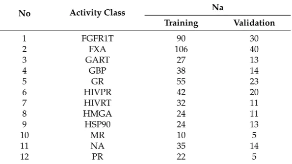
Table 2.Number of Active (Na) compounds for 12 Directory of Useful Decoys (DUD) datasets.

No Activity Class Na

Training Validation

1 FGFR1T 90 30

2 FXA 106 40

3 GART 27 13

4 GBP 38 14

5 GR 55 23

6 HIVPR 42 20

7 HIVRT 32 11

8 HMGA 24 11

9 HSP90 24 13

10 MR 10 5

11 NA 35 14

12 PR 22 5

(5)

well defined derivatives and biologically relevant compounds that were converted to Pipeline Pilot’s ECFC_4 fingerprints and folded to give 1024 element fingerprints. A detailed description of each dataset showing the training (70%) and validation (30%) sets, activity classes, number of molecules per class, and their average pairwise Tanimoto similarity across all pairs of molecules is given in Tables3–5. The active molecules for each dataset were used. For instance, the MDDR1 (Table3) contains a total of 8294 active molecules, which is a mixture of both structurally homogeneous and heterogeneous active molecules (11 classes). The MDDR2 (5083 molecules) and MDDR3 (8568 Molecules) in Tables4and5 respectively, contain 10 homogeneous activity classes and 10 heterogeneous ones respectively [27].

Table 3.Activity Classes for MDDR1.

Activity Index Activity Class Active Molecules Pairwise Similarity Training Validation Mean

31420 renin inhibitors 783 347 0.573

71523 HIV protease inhibitors 535 215 0.446

37110 thrombin inhibitors 561 242 0.419

31432 angiotensin II AT1 antagonists 674 269 0.403

42731 substance P antagonists 859 387 0.339

06233 5HT3 antagonists 530 222 0.351

06245 5HT reuptake inhibitors 257 102 0.345

07701 D2 antagonists 268 127 0.345

06235 5HT1A agonists 589 238 0.343

78374 protein kinase C inhibitors 326 127 0.323

78331 cyclooxygenase inhibitors 427 209 0.268

Activity Index Activity Class Active Molecules Pairwise Similarity Training Validation Mean

07707 adenosine (A1) agonists 136 71 0.424

07708 adenosine (A2) agonists 119 37 0.484

31420 renin inhibitors 791 339 0.584

42710 monocyclicβ-lactams 78 33 0.596

64100 cephalosporins 911 390 0.512

64200 carbacephems 115 43 0.503

64220 carbapenems 732 319 0.414

64300 penicillin 88 38 0.444

65000 antibiotic, macrolide 268 120 0.673

75755 vitamin D analogous 323 132 0.569

Activity Index Activity Class Active Molecules Pairwise Similarity

Training Validation Mean

(6)

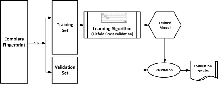
The datasets were divided into training (70%) and validation (30%) sets for the purpose of this experiment. Ten-fold cross-validation was used for the Training set. In this cross-validation, the data set was split into 10 parts; 9 were used for training and the remaining 1 was used for testing. This process is repeated 10 times with a different 10th of the dataset used to test the remaining 9 parts during every run of the 10-fold cross validation. Figure1pictorially illustrates the various stages involved in the work under study.

Molecules 2016, 21, 983 6 of 10

during every run of the 10-fold cross validation. Figure 1 pictorially illustrates the various stages involved in the work under study.

Complete Fingerprint Training Set Validation Set Trained Model Learning Algorithm

(10 fold Cross validation)

Split

Evaluation results Validation

Figure 1.Experimental Design.

3.2. Xgboost and Machine Learning Algorithms Parameters

Identifying the optimal parameters for a classifier can be time consuming and tedious and Xgboost is not an exception. This is even more challenging in Xgboost due to the wide range of tuneable parameters for optimal performance; a few of which, using the R [28] implementation of Xgboost, we have restricted our scope to in this work. Thus, by using brute force, we obtained the best performance for Xgboost when eta, gamma, minimum child weight and maximum depth were 0.2, 0.16, 5 and 16 respectively. Where; eta is the step size shrinkage meant to control the learning rate and over-fitting through scaling each tree contribution, gamma is the minimum loss reduction required to make a split, minimum child weight is the minimum sum of instance weight needed in a child and max depth is the maximum depth of a child. Other tree booster parameters like maximum delta step, subsample, column sample and the number of trees to grow per round are left at their default values of 1 respectively. For LSVM, WEKA workbench offers a way to automate the search for optimal parameters. By using grid search, a peak performance with the radial basis kernel was

obtained when gamma and cost were 5.01187233627273 × 104_{and 20 respectively. RF performed best}

when the maximum depth of tree was not constrained and the number of iteration set to its default value of 100. The NB classifier achieved best performance when kernel estimator parameter is used instead of normal distribution. For RBFN, we converted numeric attributes to nominal and set the minimum standard deviation to 0.1 to get the best performance.

3.3. EvaluationMetrics

The choice of performance evaluation for both model building and validation have been carefully selected from the most commonly used metrics in the literature. The selected evaluation metrics includes the accuracy, area under curve (AUC), sensitivity (SEN), specificity (SPC) and F-measure (F-Sc). The one run definition of AUC (Equation (11)) also known as balanced accuracy which is given by the average of the sum of sensitivity and specificity has been used in this work.

AUC = ((SEN + SPC))/2 (11)

while sensitivity (SEN) (Equation (12)) and specificity (SPC) (Equation (13)) show the ability of the model to correctly classify true positive as positive and true negative as negative respectively, AUC simply describes the tradeoff between them.

SEN = tp/(tp + fn) (12)

SPC = tn(tn + fp) (13)

Figure 1.Experimental Design.

3.2. Xgboost and Machine Learning Algorithms Parameters

Identifying the optimal parameters for a classifier can be time consuming and tedious and Xgboost is not an exception. This is even more challenging in Xgboost due to the wide range of tuneable parameters for optimal performance; a few of which, using the R [28] implementation of Xgboost, we have restricted our scope to in this work. Thus, by using brute force, we obtained the best performance for Xgboost when eta, gamma, minimum child weight and maximum depth were 0.2, 0.16, 5 and 16 respectively. Where; eta is the step size shrinkage meant to control the learning rate and over-fitting through scaling each tree contribution, gamma is the minimum loss reduction required to make a split, minimum child weight is the minimum sum of instance weight needed in a child and max depth is the maximum depth of a child. Other tree booster parameters like maximum delta step, subsample, column sample and the number of trees to grow per round are left at their default values of 1 respectively. For LSVM, WEKA workbench offers a way to automate the search for optimal parameters. By using grid search, a peak performance with the radial basis kernel was obtained when gamma and cost were 5.01187233627273ˆ104and 20 respectively. RF performed best when the maximum depth of tree was not constrained and the number of iteration set to its default value of 100. The NB classifier achieved best performance when kernel estimator parameter is used instead of normal distribution. For RBFN, we converted numeric attributes to nominal and set the minimum standard deviation to 0.1 to get the best performance.

3.3. Evaluation Metrics

The choice of performance evaluation for both model building and validation have been carefully selected from the most commonly used metrics in the literature. The selected evaluation metrics includes the accuracy, area under curve (AUC), sensitivity (SEN), specificity (SPC) and F-measure (F-Sc). The one run definition of AUC (Equation (11)) also known as balanced accuracy which is given by the average of the sum of sensitivity and specificity has been used in this work.

AUC “ ppSEN `SPCqq{2 (11)

(7)

SEN “ tp{ptp`fnq (12)

SPC “ tnptn`fpq (13)

where tp, tn, fp and fn are true positive, true negative, false positive and false negative respectively. In addition to the accuracy (Equation (14)) which is the sum of the correctly classified divided by the total number of classes, F-measure (FSc) (Equation (15)), which is the harmonic mean of precision and recall is included to serve as measure the model’s accuracy.

ACC “ pptp` tnq{ptp`tn`fn`fpqq (14)

F Sc “ 2pprecisionˆrecallq{pprecision`recallq (15)

This work aims to introduce Xgboost for activity prediction through its performance on known datasets in drug discovery. To achieve this aim, the performance of Xgboost was compared with four state of the art machine learning algorithms used in drug discovery based on the afore-stated evaluation metrics. The prediction performances of the different machine learning algorithms on the datasets under study are tabulated in Tables6–12. The best values for each metric is shaded.

Table 6.Sensitivity, Specificity, Area under Curve, Accuracy and F-measure on MDDR1 Dataset.

ML Algorithm

SEN SPC AUC ACC F-Sc SEN SPC AUC ACC F-Sc

XGB 0.9484 0.9958 0.9721 0.9575 0.9830 0.9579 0.9960 0.9769 0.9594 0.9536 RF 0.9474 0.9963 0.9718 0.9621 0.9514 0.9502 0.9957 0.9730 0.9590 0.9525 LSVM 0.9258 0.9943 0.9600 0.9425 0.9264 0.9357 0.9948 0.9653 0.9497 0.9371 RBFN 0.7566 0.9773 0.8670 0.7719 0.7451 0.7751 0.9777 0.8764 0.7746 0.7553 NB 0.7648 0.9781 0.8715 0.7826 0.7578 0.7488 0.9762 0.8625 0.7626 0.7383

ML Algorithm

(8)

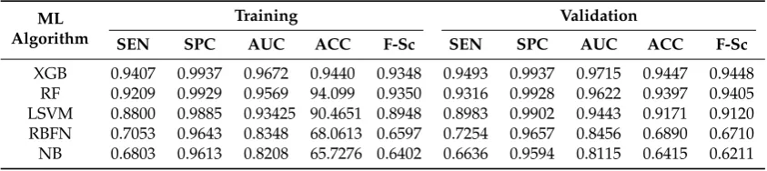
Table 9.Sensitivity, Specificity, Area under Curve, Accuracy and F-measure on DUD Dataset.

ML Algorithm

Table 10.Sensitivity, Specificity, Area under Curve, Accuracy and F-measure on COX2 Dataset.

ML Algorithm

Table 11.Sensitivity, Specificity, Area under Curve, Accuracy and F-measure on BZR Dataset.

ML Algorithm

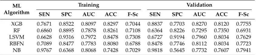
Table 12.Sensitivity, Specificity, Area under Curve, Accuracy and F-measure on ER Dataset.

ML Algorithm

The classification performance of the MDDR1-3, DUD, COX2, BZR and ER datasets are reported in Tables6–12respectively.

The experimental results on MDDR1-3 Validation datasets (Tables 6–8) shows that Xgboost produced the best accuracy, sensitivity, specificity, AUC and F-Sc across all the activity classes compared to the other machine learning methods (RF, LSVM, RBFN and NB) despite the obvious imbalance distribution of activity classes in the most of the datasets. Hence, the Xgboost method performed well for the high diverse dataset (MDDR3), and these results are particularly interesting since the MDDR3 is made up of heterogeneous activity classes which are more challenging for most machine learning algorithms.

(9)

For COX2, ER and BZR Validation datasets (Tables10–12), it is shown that Xgboost performed well and produced the best accuracy and AUC for COX2 and ER datasets. In addition, it obtained the best F-Sc results for COX2 dataset compared to the other state-of-art methods.

Visual inspection of the results shows that Xgboost produced the best accuracy for all used datasets (except for BZR dataset which produced the second best accuracy). While the performance of Xgboost on most activity classes in terms of accuracy and AUC remains the best, it still produces the best average performance across all evaluation metrics. In addition, the good performance of Xgboost is not only restricted to homogenous activity classes since it also performed well on the heterogeneous dataset.

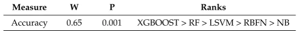
Moreover, a quantitative approach using Kendall W test of concordance was used to rank the effectiveness of all used methods as shown in Table13. This test shows whether a set of raters make comparable judgments on the ranking of a set of objects. Hence, the XGB, RF, LSVM, RBFN and NB methods were used as the raters, and the accuracy measure (using MDDR1-3, DUD, COX2, BZR and ER datasets respectively) were used as the ranked objects. The outputs of this test are the Kendall coefficient (W) and the associated significance level (p value). In this paper, if the value is significant at a cutoff value of 0.01, then it is possible to give an overall ranking for the methods.

The results of the Kendall analysis for the seven datasets are shown in Table13. The columns show the evaluation measure, the value of the Kendall coefficient (W), the associated significance level (p value), and the ranking of prediction methods. The overall rankings of the four methods show that Xgboost significantly outperforms the other methods using accuracy measure across all datasets.

Table 13.Rankings of Prediction Methods based on Kendall W Test Using Accuracy Measure.

Measure W P Ranks

Accuracy 0.65 0.001 XGBOOST > RF > LSVM > RBFN > NB

4. Conclusions

This paper investigated the performance of Xgboost on bioactivity prediction and found out that Xgboost is indeed a robust predictive algorithm. Experimental results show that Xgboost is not only effective as a predictive model for homogeneous dataset but can replicate such effectiveness on structurally heterogeneous dataset. Experimental results show that Xgboost produces an impressive predictive accuracy, ranging from 94.47% accuracy in the heterogeneous data to 98.49% in the homogeneous one. In addition to the obvious fact that Xgboost has been shown in this work to be a good predictive tool for bioactive molecule, we are hopeful that by this Xgboost would be seen as an invaluable addition to already known computational approaches to target prediction and thus leading to a wider perspective of the data rather than a single approach.

Acknowledgments: This work is supported by the Ministry of Higher Education (MOHE) and Research Management Centre (RMC) at the Universiti Teknologi Malaysia (UTM) under the Research University Grant Category (VOT Q.J130000.2528.14H75).

Author Contributions: I.M. is a researcher and conducted this project research under the supervision of F.S. All authors read and approved the final manuscript.

Conflicts of Interest:The authors declare no conflict of interest.

References

1. Johnson, M.A.; Maggiora, G.M.Concepts and Applications of Molecular Similarity; John Wiley & Sons: New York, NY, USA, 1990.

(10)

3. Yang, Z.R. Biological applications of support vector machines.Brief. Bioinform.2004,5, 328–338. [CrossRef] [PubMed]

4. Deconinck, E.; Zhang, M.H.; Coomans, D.; Vander Heyden, Y. Classification tree models for the prediction of blood-brain barrier passage of drugs.J. Chem. Inf. Mod.2006,46, 1410–1419. [CrossRef] [PubMed]

5. Svetnik, V.; Liaw, A.; Tong, C.; Culberson, J.C.; Sheridan, R.P.; Feuston, B.P. Random Forest: A Classification and Regression Tool for Compound Classification and QSAR Modeling.J. Chem. Inf. Comput. Sci.2003,43, 1947–1958. [CrossRef] [PubMed]

6. Kauffman, G.W.; Jurs, P.C. QSAR and k-nearest neighbor classification analysis of selective cyclooxygenase-2 inhibitors using topologically-based numerical descriptors.J. Chem. Inf. Comput. Sci.2001,41, 1553–1560. [CrossRef] [PubMed]

7. Koutsoukas, A.; Lowe, R.; KalantarMotamedi, Y.; Mussa, H.Y.; Klaffke, W.; Mitchell, J.B.; Glen, R.C.; Bender, A. In silico target predictions: Defining a benchmarking data set and comparison of performance of the multiclass naïve bayes and parzen-rosenblatt window.J. Chem. Inf. Mod.2013,53, 1957–1966. [CrossRef] [PubMed]

8. Krenker, A.; Kos, A.; Bešter, J.Introduction to the Artificial Neural Networks; INTECH Open Access Publisher: Rijeka, Croatia, 2011.

9. Lavecchia, A. Machine-learning approaches in drug discovery: Methods and applications.Drug Discov. Today 2015,20, 318–331. [CrossRef] [PubMed]

10. Wolpert, D.H. The supervised learning no-free-lunch theorems. InSoft Computing and Industry; Springer: London, UK, 2002; pp. 25–42.

11. Friedman, J.H. Greedy function approximation: A gradient boosting machine.Ann. Stat.2001,29, 1189–1232. [CrossRef]

12. Adam-Bourdarios, C.; Cowan, G.; Germain-Renaud, C.; Guyon, I.; Kégl, B.; Rousseau, D. The Higgs Machine Learning Challenge.J. Phys. Conf. Ser.2015. [CrossRef]

13. Phoboo, A.E. Machine Learning wins the Higgs Challenge. CERN Bull. 2014. Available online: http://cds.cern.ch/journal/CERNBulletin/2014/49/News%20Articles/1972036 (accessed on 24 April 2016). 14. Harper, G.; Bradshaw, J.; Gittins, J.C.; Green, D.V.; Leach, A.R. Prediction of biological activity for high-throughput screening using binary kernel discrimination.J. Chem. Inf. Comput. Sci.2001,41, 1295–1300. [CrossRef] [PubMed]

15. Chen, T.; Guestrin, C. Xgboost: A Scalable Tree Boosting System.arXiv:1603.027542016. [CrossRef] 16. Chang, C.-C.; Lin, C.-J. LIBSVM: A library for support vector machines.ACM Trans. Intell. Syst. Technol.

2011,2, 27. [CrossRef]

17. John, G.H.; Langley, P. Estimating Continuous Distributions in Bayesian Classifiers. In Proceedings of the Eleventh Conference on Uncertainty in Artificial Intelligence, Montreal, QC, Canada, 18–20 August 1995. 18. Bugmann, G. Normalized Gaussian radial basis function networks. Neurocomputing1998, 20, 97–110.

[CrossRef]

19. Sutherland, J.J.; O’Brien, L.A.; Weaver, D.F. Spline-Fitting with a Genetic Algorithm: A Method for Developing Classification Structure´Activity Relationships.J. Chem. Inf. Comput. Sci.2003,43, 1906–1915. [CrossRef] [PubMed]

20. Helma, C.; Cramer, T.; Kramer, S.; de Raedt, L. Data Mining and Machine Learning Techniques for the Identification of Mutagenicity Inducing Substructures and Structure Activity Relationships of Noncongeneric Compounds.J. Chem. Inf. Comput. Sci.2004,44, 1402–1411. [CrossRef] [PubMed]

21. Huang, N.; Shoichet, B.K.; Irwin, J.J. Benchmarking sets for molecular docking. J. Med. Chem. 2006,49, 6789–6801. [CrossRef] [PubMed]

22. Al-Dabbagh, M.M.; Salim, N.; Himmat, M.; Ahmed, A.; Saeed, F. A Quantum-Based Similarity Method in Virtual Screening.Molecules2015,20, 18107–18127. [CrossRef] [PubMed]

(11)

24. BIOVIA. MDDR. Retrieved 15–07, 2015. Available online: http://accelrys.com/products/databases/ bioactivity/mddr.html (accessed on 15 July 2015).

25. Abdo, A.; Saeed, F.; Hamza, H.; Ahmed, A.; Salim, N. Ligand expansion in ligand-based virtual screening using relevance feedback.J. Comput. Aided Mol. Design2012,26, 279–287. [CrossRef] [PubMed]

26. Abdo, A.; Leclère, V.; Jacques, P.; Salim, N.; Pupin, M. Prediction of New Bioactive Molecules using a Bayesian Belief Network.J. Chem. Inf. Model.2014,54, 30–36. [CrossRef] [PubMed]

27. Hert, J.; Willett, P.; Wilton, D.J.; Acklin, P.; Azzaoui, K.; Jacoby, E.; Schuffenhauer, A. New methods for ligand-based virtual screening: Use of data fusion and machine learning to enhance the effectiveness of similarity searching.J. Chem. Inf. Mod.2006,46, 462–470. [CrossRef] [PubMed]

28. The R Core Team. R: A Language and Environment for Statistical Computing; R Foundation for Statistical Computing: Vienna, Austria, 2013.

Sample Availability:Not Available.