Bayesian Analysis and Matching Errors in Closed Population Capture Recapture Models

(1)

GOSKY, ROSS MATTHEW. Bayesian Analysis and Matching Errors in Closed Population Capture Recapture Models. (Under the direction of Leonard Stefanski and Sujit Ghosh.)

Capture-Recapture models are used to estimate the unknown sizes of animal popu-lations. When the population is closed, with constant size, during the study, eight standard models exist for estimating population size. These models allow for variation in animal cap-ture probabilities due to time effects, heterogeneity among animals, and behavioral effects after the first capture. Our research focuses on two areas:

1. Using Bayesian statistical modeling, we present versions of these eight models. We explore the use of Akaike’s Information Criterion (AIC), and the Deviance Informa-tion Criterion (DIC) as tools for selecting the appropriate model for a given dataset. Through simulation, we show that AIC performs well in model selection.

(2)

by

Ross M. Gosky

A dissertation submitted in partial satisfaction of the requirements for the degree of

Doctor of Philosophy

in

STATISTICS

in the

GRADUATE SCHOOL at

NC STATE UNIVERSITY

2004

Leonard Stefanski, Co-Chair Sujit Ghosh, Co-Chair

(3)

Recapture Models

by

(4)

(5)

Biography

(6)

Acknowledgements

I would like to thank my family for their love and support during the past five years. The last five years at NC State have been wonderful for me. Becky and Ryan have supported me so much during this time and have helped me immeasurably. Becky has been my best friend through this, and Ryan never fails to bring a smile to my face and helps me to keep everything in proper perspective.

My advisors, Len Stefanski and Sujit Ghosh, have been of immense help through-out the development of this thesis. They are excellent statisticians and people, and I am fortunate to have learned from them.

I would like to thank Harsha Rao and Terry Byron for their help with any and all computing questions (there were many) and for being good friends as well.

Many graduate students have also helped me very much with their friendship and advice. Although I am certain to miss many names, some of these people are Kevin Daly, Steve Hoffner, Jimmy Doi, Jared Lunceford, Jeff Burnett, Doug Robinson, Julie McIntyre, Clay Barker, Jing Wang, Hyeyoung Lee, Michael Crotty, Alvin Van Orden, Tae-Young Heo, Palani Ravindran, Shaw Yoshitani, Karen Chiswell, Michael Crotty, Joe Boyer, Prasheen Agarwal, Katja Remlinger, and Sheng Feng.

My committee members, Ken Pollock and Cavell Brownie, have been very helpful with this research and thesis. Ken was very instrumental in helping frame the topic, and his time and efforts are greatly appreciated.

(7)

List of Figures

2.1 Experiment 2 Posterior Median and AIC Results (True N = 500) . . . 42

2.8 Posterior density of N for model M0 for Cottontail dataset . . . 66

2.9 Posterior density of N for model Mh for Cottontail dataset . . . 66

3.1 Simulation Results for T = 25 when q1 =q2 . . . 92

3.2 Simulation Results for T = 25 when q1 6=q2 . . . 93

3.3 Simulation Results for T = 50 when q1 =q2 . . . 95

3.4 Simulation Results for T = 50 when q1 6=q2 . . . 96

3.5 Simulation Results for T = 100 when q1=q2 . . . 97

(10)

List of Tables

2.1 Parameters in Bayesian Closed Population Capture-Recapture Models . . . 19

2.2 Data generating assumptions for each of the 8 Bayesian models for simula-tion experiment one. F refers to the Logistic distribusimula-tion funcsimula-tion F(x) = [1 +e−x_]−1 , µ = F−1_{(0.2) =} ₋_1.39, _κ _{= 1.25,} _z i i.∼i.d. N(0,1), η = 1, and φj = j−₂3, j= 1,2, ...,5 . . . 20

2.3 Means and Standard Errors of Posterior Median as an estimator of N (True N = 500; Number of Simulations 100; Standard Errors given in parentheses) 23 2.4 Coverage Probability of ˆN from 95 percent Equal Tail Posterior Interval (TrueN = 500) . . . 23

2.5 Means and Standard Errors of AIC Posterior Mean . . . 29

2.6 AIC Model Selection: Percentage of times each model selected . . . 30

2.7 Means and Standard Errors of DIC . . . 33

2.8 DIC Model Selection: Percentage of times each model selected . . . 34

2.9 mean values of pD: ¯D(θ) - D(ˆθ) . . . 34

2.10 Means and Standard Errors of DIC: when posterior median used for ˆθ . . . 35

2.11 mean values of pD: ¯D(θ) - D(ˆθ) where ˆθ is the Posterior Median . . . 36

2.12 DIC Model Selection: Percentage of times each model selected when posterior medians used for ˆθ . . . 36

2.13 Data generating assumptions for simulation experiments 1 to 8 . . . 38

2.14 Calculations ofpij for simulation experiments 1 to 8; F refers to the Logistic distribution functionF(x) = [1 +e−x_]−1 ,Zi i.∼i.d.N(0,1),τij = 1 if the animal has been previously captured, and τij = 0 otherwise; values of µ, η, φj, and κ are given in Table 2.15 . . . 38

2.15 Design specifications for simulation experiments 1 to 8 . . . 39

2.16 Average Capture Probabilities, and their Standard Deviations, for Simulation Experiments 1 to 8 . . . 40

2.17 Selection Rates for AIC for Simulation Experiments 2 to 8 . . . 63

2.18 Program CAPTURE Results for Cottontail data set (first 5 capture periods) 65 2.19 Bayesian Model Results for Cottontail data set (first 5 capture periods) . . 65

(11)

2.21 Means and Standard Errors of AIC: Experiment 2 . . . 68 2.22 Means and Standard Errors of Posterior Median: Experiment 3 (TrueN =

500) . . . 69 2.23 Means and Standard Errors of AIC: Experiment 3 . . . 69 2.24 Means and Standard Errors of Posterior Median: Experiment 4 (TrueN =

100) . . . 74 2.33 Means and Standard Errors of AIC: Experiment 8 . . . 74 3.1 Notation for the two-stage bootstrap procedure. Two-stage bootstrap

pa-rameters, observed data, and estimated and predicted quantities for each stage. . . 86 3.2 Bootstrap Prediction Interval Results: Simulated Coverage Probabilities and

(12)

Chapter 1

Closed Population Capture

Recapture Models

(13)

the first sample is taken, subsequent samples return a combination of marked and unmarked animals. When several samples are taken, different tags (or the same tag with a unique identifier) are used for each sample so that a distinct capture history is available for all the captured animals in the population. The goal is to use the percentages of recaptured animals as a basis for estimating the number of animals that were never captured during the study. This number of animals which are non-captured (which is estimated) plus the number that were captured during at least one of the captures forms an estimate ˆN of the population size N. When this methodology is applied to lists of people, each separate list is considered a separate capture and the information from the separate lists is used to estimate the population size N.

Denoting the number of capture periods for the study as k, we can examine the simple case where there are k= 2 captures from the population.

Denoting

n1 = number of captured animals in capture period 1 n2 = number of captured animals in capture period 2 m2 = number of recaptured animals in capture period 2

the most common estimator forN is

ˆ

N = n1n2 m2

. (1.1)

(14)

hypergeo-metric or multinomial likelihood functions which condition onn1, and is a commonly-used estimator of population size.

A more general set of models with possibly k >2 captures using the multinomial distribution are also available. A good introduction to these models is presented by Otis, Burnham, White, and Anderson (1978). We introduce the details of their general framework here, which is used throughout the rest of the thesis. Define indicator variablesXij as

Xij = 1 if animali is captured during capture periodj

fori= 1,2, ..., N andj = 1,2, ..., k. Also denote

pij = Pr (Xij = 1)

as the probability that animal iis captured during capture period j. Denote the capture matrixX with dimensionsN_×kwith entryX[i, j] =Xij in rowiand columnj. Denoting

X[i, .] as theithrow of X, we note that this vector has 2k_{possible values, as each entry in}

the vector must be zero or one. For notational simplicity, these outcomes can be ordered as

Outcome 0: capture history (0,0,0, ...,0,0,0);

(15)

through

Outcome 2k₋_{1: capture history (1,}_1,_{1, ...,}_1,_1,_1).

Each animal in the population has exactly one of the 2k _{capture histories. A mathematical}

representation of the above outcomes is obtained through the notation (Xi1, Xi2, ..., Xik)

of kvalues to represent the observed capture history of any animal in the population. For l = 0,1,2, ...,2k₋_{1, we define Capture History} _L _{corresponding to the previous ordering}

of outcomes, where L = Pk_j₌₁Xij2k−j. When necessary to refer to the capture history

of animal i, we denote the capture history of animal i as capture history Li, where Li = Pk

j=1Xij2k−j. Denote the matrix Y with dimensions N ×2k, with entry Y[i, l] = 1 if

animal i has capture history outcome Li −1 from the list of outcomes above. That is,

Y[i,1] = 1 if animal i has capture history (0,0, ...,0), Y[i,2] = 1 if animal i has capture history (0,0,0, ...,0,1), etc. Exactly one entry in the vector Y[i, .] is equal to 1, the rest of the entries in the vector are zero. DenoteZL=PNi=1Y[i, l+1] as the number of animals with capture historyL, forL= 0,1, ...,2k₋_{1. Notice that}_Z

0cannot be observed, as it represents the number of animals with capture history (0,0, ...,0). Notice also that P2_l₌₀k−1Zl = N.

Denote S = P2k−1

l=1 Zl = N −Z0 as the number of animals observed during at least one capture period. Note also thatZl =PNi=1I(li =l).

We can compute the probability of animal ihaving capture history li (denoted as

Pli) as

Pli =

k Y

j=1 pxij

ij (1−pij)1−xij (1.2)

(16)

L= 2k₋_{1 and}_P

l=QNi=1P

I(li=l)

li then the likelihood function can be written as

L(N, P_|Z1 =z1, ..., ZL=zL) =

N!

(N₋S)!QL_l₌₁Zl! L Y

l=1 PZl

l Ã

1₋

L X

l=1 Pl

!N−S

. (1.3)

Notice that ifN were known, this model would represent a multinomial likelihood function with counts Z0, ..., Z2k₋₁ and probabilities P₀, ..., P₂k₋₁. A set of assumptions underlying

this modeling structure are (Otis et al. (1978)):

1. The population is closed (no births, deaths, or migrations during the study);

2. Animals retain their tags throughout the experiment;

3. All tags/marks are correctly noted after each capture.

(17)

1.0.1 Background for Our Approaches to Bayesian Modeling and

Match-ing Errors

When the three listed assumptions are valid, we use Bayesian inference and model selection procedures. In Otis et al. (1978), a set of eight closed population models are proposed. We present Bayesian versions of these models and use model selection criteria to select the best model for a given dataset. Each model makes different assumptions about the complexity of the capture probabilities pij. Brief summaries of the model types follow.

Model M0: pij is constant for alli, j.

Capture probabilities are constant for all individuals and all capture periods.

Model Mt: The subscript tdenotes time effects in the model.

pij varies by capture period (that is, by j), but not by individuals.

Model Mh: The subscripth denotes heterogeneity in the population.

pij varies by individual but not by capture period. This is often a realistic assumption,

as some animals may be easier to capture than others (for example, the probability of capturing an animal may be different for animals of different ages).

Model Mb: The subscript bdenotes a behavioral effect in the population.

(18)

Model Mth: Use of two or more subscripts indicates the presence of both effects. Here,pij

varies both by individual (byi) and by capture period (byj).

Model Mtb: As the subscript b indicates, a trap effect is assumed after the initial

cap-ture, but we also assume that different capture periods may have different capture probabilities (that is, vary byj).

Model Mbh: Capture probabilities vary by animal (by i). And, a trap effect is assumed

after first capture.

Model Mtbh: Combines all three types of effects. Capture probabilities vary by capture

period, by individual, and a trap effect is assumed.

In Model M0, one assumes that pij are constant across all time periods and all

animals. That is, pij =p, where p is constant. To incorporate time effects for Model Mt,

one can assumepij =pj. Similarly, behavioral effects for ModelMb can be incorporated by

using ofpij =pB if the animal has not been captured before capture periodj, andpij =pA

if the animal has been captured before capture period j.

Models with heterogeneity present a challenge to the form of the likelihood we have defined previously. Under heterogeneity models,pij may vary withi. This could cause

Pli to vary by i as well. Our likelihood function assumes that Pli do not vary with i. If

(19)

be noted that in Link (2003), inference about N in heterogeneity models is shown to be highly model-dependent, suggesting that careful consideration in required when accounting for heterogeneity in capture-recapture models.

Program CAPTURE (described in Otis et al. (1978)), provides estimators of N for some the above models. Additionally, it provides model selection functionality based on Chi-Square goodness of fit tests. The models and estimators of N used in program CAPTURE are as follows:

M0: basic M0 model estimator

Mh: uses jackknife estimator (Burnham and Overton, 1978)

Mb: uses Zippin removal estimator (Zippin, 1956)

Mt: uses Darroch estimator (Darroch, 1958)

Mbh: uses a generalized removal estimator (see Seber, 1982)

Mtb: uses an estimator from Burnham (unpublished)

Mth: uses Chao estimator (Chao, et al, 1992)

Mtbh: not available in Program CAPTURE

(20)

Another form of model selection occurs when experimenters have basic beliefs about the population that may logically eliminate one or more of the models from consid-eration. However, the removal of potentially appropriate models based upon assumptions about the population would be a danger to this approach. For these reasons, further work on model selection criteria is needed.

The work we present in this thesis is separated into two different topics:

Bayesian Models and Model Selection for Closed Population Models .

We present Bayesian versions of the above models, utilizing a mixture approach to modeling heterogeneity, and allowing for fixed time and behavioral effects in the ap-propriate models. Furthermore, through extensive simulations, we explore the use of Akaike’s Information Criterion (AIC) and also the Deviance Information Criterion (DIC) as potential model selection criteria.

Effects of Matching Errors in Closed Population Models .

(21)

(22)

Chapter 2

Bayesian Estimation and Model

Selection for Closed Population

Models

2.1 Introduction and Motivation for Model Selection

Proce-dures

Analysis of Capture-Recapture data for closed populations typically uses one of the eight standard models mentioned in Chapter 1. Some definitive methods surrounding selection of the correct model is necessary in such analyses. The eight models are gener-ally (though not exclusively) nested, ranging from very simple models (M0) where capture probabilities are equal for all animals across all capture periods, to complex models (Mtbh)

(23)

effects. In such situations, model selection criteria are critical to allow the best model of the eight to be fit to the data. Following the researcher’s suspicions about which model to use may lead to choice of a model which is too simple to fit the data. Similarly, although it is tempting to choose the most complex model to analyze the data, this may lead to over-fitting and hence a higher predictive variance. The desire to strike a balance between choice of a model that neither under-fits nor over-fits the data is the motivation for model selection criteria (Burnham, 2002, chap.1).

Akaike’s Information Criterion (AIC) is one such method of model selection, and seems to be the most commonly used measure for model selection. The intent of AIC is to measure the mathematical distance between the true population and the fitted model, by using the so-called Kullback-Leibler discrepancy. To differentiate between models with different number of parameters, AIC adds two times the number of model parameters to the estimated Kullback-Leibler discrepancy. In a case where there are two models, one simple and the other complex, that fit a data set equally well, this allows AIC to choose the simpler model by penalizing the complex models. Generally the rule of parsimony says that a researcher should choose the simplest model that describes the behavior of the population. Use of AIC generally supports this rule.

(24)

estimation.

The Deviance Information Criterion (DIC) is a Bayesian model selection crite-rion (Speigelhalter, Carlin, et al 2002). It is structured similarly to AIC, but is strictly a Bayesian criterion. The main difference between AIC and DIC is in the penalty term added to the estimated Kullback-Leibler discrepancy. DIC adds two times the effective number of parameters to the estimated Kullback-Leibler discrepancy. The effective number of param-eters is a Bayesian concept. It deals with the fact that the number of model paramparam-eters in a Bayesian model is influenced by their prior distributions. The DIC criterion presents a methodology to measure this number of parameters. The DIC is, then, the difference between the estimated mean KL distance, and the KL distance estimated at the posterior mean of each of the model parameters.

We also examine DIC as a model selection criterion for these models. Use of DIC does not require the models to be nested. However, as we will see, our modeling uses a mixture approach for some of the models. There are some questions about use of DIC for mixture models.

We considered using the Bayesian Information Criterion (BIC) for model selection, but, for capture-recapture models it is not clear what the sample size should be (asN itself is a parameter andk, the number of capture periods, is usually much smaller than necessary for asymptotic properties to work). Therefore, we chose to focus on AIC and DIC as the two model selection criteria to be examined.

Specifically, our goals are to answer the following questions:

(25)

(ii) Similarly, how does DIC perform as a model selection criterion for these models?

(iii) Are one or more of the eight closed population models particularly robust when fitting data generated under a different model structure?

To assess this, we develop and present Bayesian versions of the eight standard closed popu-lation capture-recapture models. We present simupopu-lation results to determine whether AIC and DIC work well in differentiating between the models.

2.2 Bayesian Closed Population Capture Recapture Models

We use the general framework outlined in Chapter 1. For each model, the following notation is common. N represents the (unknown) population size. We usepij,Pl, Zl, and

S as previously defined in Chapter 1.

The set of sufficient statistics is given by_{Z1, Z2, . . . , ZL} whereL= 2k−1.

Esti-matingN is equivalent to estimatingZ0, the number of individuals in the population which were undetected during the study. UsingPlas defined in Chapter 1, letP = (P1, P2, . . . , PL).

We can thus obtain the likelihood function as L(N, P)

L(N, P)_∝

Ã

N S

! _L

Y

l=1 Pzl

l Ã

1₋

L X

l=1 Pl

!N−S

. (2.1)

(26)

estimates. For each of the eight models we use the following prior distribution forN,

P r(N =n)_∝ 1

nδ, n= 1,2, ...., Nmax

whereδ >0 is fixed at a specific value andNmaxis set at a realistic upper bound forN. The

Jeffreys prior can be approximated with δ = 1₂, which we use for our simulations (results given in Section 2.3). Now we describe the basic modeling of these capture probabilities for each of the eight models and associated prior distributions for model parameters.

Model M0: pij =α for alli, j.

We use a Beta distribution for α, specifically α _∼ Beta(a, b). For our simulations (discussed in Section 2.3), we fixed a=b= 0.5.

Model Mt: pij =αj for all i.

We use a sequence of independent and identically distributed (i.i.d.) Beta random variables for αj’s, specifically, αj i.∼i.d. Beta(a, b). For our simulations (Section 2.3),

we fixed a=b= 0.5.

Model Mh: pij =pi for all j, and pi ∼F(·).

To account for heterogeneity, we assume a finite mixture distribution for univariate distribution function,F, specifically the probability mass function (p.m.f.) is given by dF(p) =Prm=1πmI(p=θm), where πm denotes the probability at support point θm

with the restriction that Pr_m₌₁πm = 1. It has been shown that when using mixture

(27)

our simulations (Section 2.3), we fix r = 2 mass points representing possibly two distinct groups within the population. One group represents a relatively easier group to capture, and the second a relatively more difficult group to capture. As this is a mixture model, some extra restrictions are needed to allow all the parameters in the model to be identified. In our mixture model, we imposed an order restriction on θ1, θ2 to forceθ1≤θ2. To do this, we createdθ1∗, θ∗2, π

i.i.d.

∼ Beta(a, b). The probability

at the r = 2 support points is given by 1₋π2 = π1 =π. Our order restriction sets θ1=M in(θ1∗, θ∗2). Similarly, θ2=M ax(θ1∗, θ∗2). For our simulations (Section 2.3), we fixeda=b= 0.5.

Model Mb: pij =αI(τij = 0) +βI(τij = 1)

where τij = 1 if animal i has been captured before capture period j, and τij = 0

otherwise. This means that a trap-effect is assumed after the first capture. Subsequent captures are assumed not to cause such an effect. We use α, β i._∼i.d.Beta(a, b) as the prior distributions. For our simulations (Section 2.3), we fixed a=b= 0.5.

Model Mth: pi= (pi1, pi2, . . . , pik)T ∼F(·).

Similar to anMhmodel, we assume a finite mixture distribution for thek-dimensional

distribution function, F, specifically the p.m.f. is given by

dF(p) =Prm=1πmI(p=θm), whereπm denotes the probability at support point

θm = (θ1m, . . . , θkm)T with the restriction that Prm=1πm = 1. For our simulations

(Section 2.3), we fix r = 2 mass points representing possibly two distinct groups within the population, which means that 1₋π2 =π1 =π. We impose similar order restrictions as in Mh on the parameters θ1j, θ2j. That is, π, θ₁∗j, θ2∗j

i.i.d.

(28)

θ1j =M in ³

θ∗

1j, θ2∗j ´

, and θ2j =M ax ³

θ∗

1j, θ∗2j ´

forj = 1, . . . , k. For our simulations (Section 2.3), we fixeda=b= 0.5.

Model Mtb: pij =βjI(τij = 1) +αjI(τij = 0).

where τij is as defined in model Mb. As in model Mb, the trap effect is assumed to

occur only after initial capture but now allowed to vary over capture periods. For j = 1,2, ..., k, define αj as the capture probabilities for capture period j for animals

that have not been previously captured. For j = 2,3, ..., k, define βj as the capture

probabilities for animals that have been captured prior to capture periodj. Note that β1 is undefined, because subsequent capture cannot occur in the first capture period, so we fix β1 = 0. In addition, we assume that βj = αj +c, for j = 2, . . . , k We use

αj i .i.d.

∼ Beta(a, b) as the prior distribution for α’s. The conditional prior distribution

of c, given α2, ..., αj is U(−min2≤j≤kαj,1−max2≤j≤kαj), where U(a, b) denotes a

uniform distribution over (a, b).

Model Mbh: pij =p1iI(τij = 0) +p2iI(τij = 1) andpi = (p1i, p2i)T ∼F(·)

where τij is as defined in model Mb. Similar to the Mh model, we assume a

fi-nite mixture distribution for the 2-dimensional distribution function, F, specifically dF(p) =Pr_m₌₁πmI(p=θm), whereπm denotes the probability at support point

θm = (θ1m, θ2m)T with the restriction that Prm=1πm = 1. For our simulations

(Sec-tion 2.3), we fixr = 2 mass points representing possibly two distinct groups within the population, which means that 1₋π2 =π1=π∼Beta(a, b). Again, we impose order restrictions on theθparameters for convergence and useπ, θ∗

1m, θ∗2m

i.i.d.

∼ Beta(a, b) for

(29)

Similarly, we set θ21 =M in(θ∗

21, θ22∗ ), and θ22=M ax(θ∗21, θ22∗ ). For our simulations (Section 2.3), we fixeda=b= 0.5.

Model Mtbh: pi = (pi1, . . . , pi2)T =p(1)i I(τij = 0) +p(2)i I(τij = 1) and (p(1)i , p

(2)

i )∼F(·).

This is the most general model that allows effects for individual heterogeneity, time, and behavior. Similar toMbhandMthmodels, we assume a finite mixture distribution

for the 2k-dimensional distribution function,F, specifically that

dF(p) = Pr_m₌₁πmI(p = θm), where πm denotes the probability at support point

θm= (θ11m, . . . , θ1km, θ21m, . . . , θ2km)T with the restriction thatPrm=1πm = 1. As in

model Mtb, we set the behavior effect to be additive. That is, θ2jm = θ1jm +c for

j = 2, ..., k and m = 1,2, ..., r. For our simulations (Section 2.3), we fix r = 2 mass points representing possibly two distinct groups within the population, which means that 1₋π2 =π1 = π. Prior distributions for π and θ1jm are π, θ₁∗jm

i.i.d.

∼ Beta(a, b)

for j = 1, . . . , k and m = 1,2. A conditional prior distribution of c given θ1jm for

j = 1, . . . , k and m = 1,2 is U(₋min2≤j≤kθ1jm,1−max2≤j≤kθ1jm), where U(a, b)

denotes a uniform distribution over (a, b). Notice that this implies the behavioral effect c is constant across the m groups within the population. Also, we imposed similar order restrictions as in the previous heterogeneity models, so thatθ1j1 ≤θ2j1 and θ1j2≤θ2j2. For our simulations (Section 2.3), we fixed a=b= 0.5.

(30)

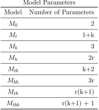
Model Parameters Model Number of Parameters

M0 2

Mt 1+k

Mb 3

Mh 2r

Mtb k+2

Mbh 3r

Mth r(k+1)

Mtbh r(k+1) + 1

Table 2.1: Parameters in Bayesian Closed Population Capture-Recapture Models

1) +kr+ 1 = r(k+ 1) + 1. The other entries in Table 2.1 can be established in a similar fashion.

The posterior distributions of the model parameters for all eight models can be closely approximated using Markov Chain Monte Carlo (MCMC) methods available in the WinBUGS V1.4 software package

(http://www.mrc-bsu.cam.ac.uk/bugs/winbugs/contents.shtml).

2.3 A Simulation Study

2.3.1 Data Generation Process

(31)

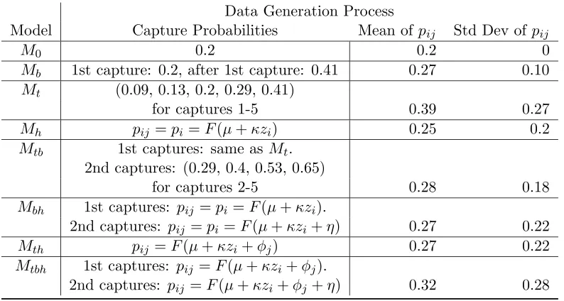
Data Generation Process

Model Capture Probabilities Mean of pij Std Dev of pij

M0 0.2 0.2 0

Mb 1st capture: 0.2, after 1st capture: 0.41 0.27 0.10

Mt (0.09, 0.13, 0.2, 0.29, 0.41)

for captures 1-5 0.39 0.27

Mh pij =pi=F(µ+κzi) 0.25 0.2

Mtb 1st captures: same as Mt.

2nd captures: (0.29, 0.4, 0.53, 0.65)

for captures 2-5 0.28 0.18

Mbh 1st captures: pij =pi =F(µ+κzi).

2nd captures: pij =pi =F(µ+κzi+η) 0.27 0.22

Mth pij =F(µ+κzi+φj) 0.27 0.22

Mtbh 1st captures: pij =F(µ+κzi+φj).

2nd captures: pij =F(µ+κzi+φj+η) 0.32 0.28

Table 2.2: Data generating assumptions for each of the 8 Bayesian models for simulation experiment one. F refers to the Logistic distribution function F(x) = [1 +e−x_]−1

, µ = F−1_{(0.2) =}₋_1.39,_κ_{= 1.25,}_z

i i .i.d.

∼ N(0,1), η = 1, andφj = j−₂3, j= 1,2, ...,5

we generated 100 data sets under each modeling assumption

(M0, Mt, Mh, ..., Mtbh). Using Markov Chain Monte Carlo (MCMC) methods, we fit each

data set using each of the eight models. A total of one-hundred data sets generated under each of the eight modeling assumptions gives a total of eight-hundred data sets. Each data set is a simulated capture-recapture study withk= 5 capture periods. For each simulated data set discussed in this section, we set N = 500, and the pij values were generated

(32)

For each data set, and under each model, an estimate of the posterior density of N was constructed using WinBUGS Version 1.4 software, and the median of this posterior distribution was chosen as an estimate ofN. We also computed the AIC (Section 2.3.3), and the coverage probability of a 95 % equal-tailed interval from the posterior distribution of N by computing the 2.5th and 97.5th percentile ofN, and these results follow in Table 2.4. When fitting our models to the generated data sets, we made no assumptions about the capture probabilities being small or large. Using a large range of the prior distribution of N sufficiently allows for capture probabilities to be large or small. However, the range of N would be specific to each study.

We used a burn-in period of 3000 samples, and 2000 samples from each of three MCMC chains with dispersed starting values for the model parameters. Therefore, our posterior distribution estimates are based upon 6000 total samples.

Results of the first simulation experiment are given in Tables 2.3 - 2.12. Each ta-ble’s columns correspond to the data generating process, that is, which model’s assumptions were used to generate the data. Each table’s rows correspond to the model fit to the data. For example, the first row and fourth column of any table correspond to data generated under model Mb, but analyzed using modelM0. Similarly, the fourth row and first column represents performance ofM0 data sets analyzed using ModelMb.

(33)

and standard errors of the MCMC estimates of DIC. Table 2.8 gives the percentages of times each model was selected by DIC, out of the 100 data sets generated under each set of modeling assumptions. Table 2.9 gives the mean values of the MCMC estimates of the penalty term in DIC, as a means to assess the effective number of parameters in DIC. Further description of the DIC criterion is given in Section 2.3.4. Tables 2.10, 2.11, and 2.12 give the same corresponding results as in Tables 2.7, 2.8, and 2.9, with the difference between tables arising because different estimators of the model parameters were used for each group of tables. These different estimators are discussed in Section 2.3.4.

2.3.2 Estimation of Population Size N

For estimating N, simulation results are given in Table 2.3. Estimated coverage probabilities for a 95% equal-tailed posterior interval from the posterior distribution ofN is seen in Table 2.4.

Because we expect a fitted model to estimate N accurately when the data ana-lyzed are sampled from the true model (for example, fitting Model Mth to data generated

with time and heterogeneity effects), we expect the estimation of N to be accurate on the diagonals of each of the above tables, as the diagonals represent cases where the data gen-erating assumptions match the model used to fit the data. Secondly, we expect that a fitted model would accurately estimateN when fit to data generated under simpler assumptions, specifically when the simpler model can be viewed as a special case of the more complex model. For example, data generated under model M0 with constant capture probability across all captures, should fit well when analyzed with a model such as Mth, which allows

(34)

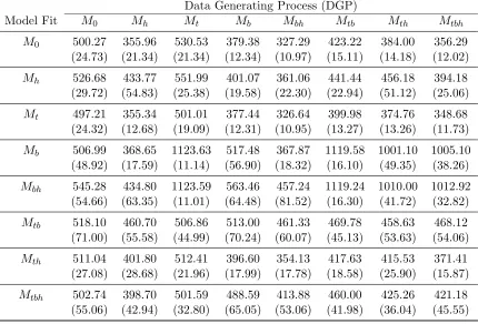
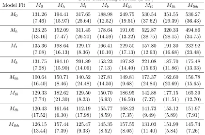
Table 2.3: Means and Standard Errors of Posterior Median as an estimator of N (True N = 500; Number of Simulations 100; Standard Errors given in parentheses)

Data Generating Process (DGP)

Model Fit M0 Mh Mt Mb Mbh Mtb Mth Mtbh

M0 500.27 355.96 530.53 379.38 327.29 423.22 384.00 356.29 (24.73) (21.34) (21.34) (12.34) (10.97) (15.11) (14.18) (12.02) Mh 526.68 433.77 551.99 401.07 361.06 441.44 456.18 394.18

(29.72) (54.83) (25.38) (19.58) (22.30) (22.94) (51.12) (25.06) Mt 497.21 355.34 501.01 377.44 326.64 399.98 374.76 348.68

(24.32) (12.68) (19.09) (12.31) (10.95) (13.27) (13.26) (11.73) Mb 506.99 368.65 1123.63 517.48 367.87 1119.58 1001.10 1005.10

(48.92) (17.59) (11.14) (56.90) (18.32) (16.10) (49.35) (38.26) Mbh 545.28 434.80 1123.59 563.46 457.24 1119.24 1010.00 1012.92

(54.66) (63.35) (11.01) (64.48) (81.52) (16.30) (41.72) (32.82) Mtb 518.10 460.70 506.86 513.00 461.33 469.78 458.63 468.12

(71.00) (55.58) (44.99) (70.24) (60.07) (45.13) (53.63) (54.06) Mth 511.04 401.80 512.41 396.60 354.13 417.63 415.53 371.41

(27.08) (28.68) (21.96) (17.99) (17.78) (18.58) (25.90) (15.87) Mtbh 502.74 398.70 501.59 488.59 413.88 460.00 425.26 421.18

(55.06) (42.94) (32.80) (65.05) (53.06) (41.98) (36.04) (45.55)

Table 2.4: Coverage Probability of ˆN from 95 percent Equal Tail Posterior Interval (True N = 500)

Data Generating Process (DGP) Model Fit M0 Mh Mt Mb Mbh Mtb Mth Mtbh

M0 95 0 69 0 0 0 0 0

Mh 93 69 61 95 16 98 87 37

Mt 95 0 97 0 0 0 0 0

Mb 97 2 0 93 1 0 0 0

Mbh 99 83 0 94 92 0 0 0

Mtb 98 99 94 98 99 72 80 86

Mth 95 32 97 22 5 21 33 1

(35)

Mth is sufficiently robust to perform well in this situation because M0 can be viewed as a

special case ofMth.

Because the tables have been arranged with the complexity of the models in roughly increasing order, entries below the diagonal indicate situations where the model fit is more complex than the data generating assumptions. We generally expect to see ac-curate estimation of N in these situations. We expect less accuracy in estimating N when the column number is larger than the row number, as this (generally) represents situations where the data contain more effects than the model to which it was fit.

The results in Table 2.3 give some insights into estimation of N. Firstly, notice that when the data are generated from modelM0 (entries in column one of the table), that all the models exceptMbh provide estimates ofN with little to no bias. Model Mbh has a

relative bias of +0.10. There is some slight bias to modelsMtband modelMh(with relative

biases of +0.04 and +0.05, respectively), but overall performance is pretty good for simple data.

Data generated under model Mh (column two of Table 2.3) show that none of

the eight models estimate N particularly well for these data sets. The smallest bias in estimatingN came from ModelMtb, with a relative bias of -0.08. We expected a reasonable

estimate ofN would be provided by at least the four models which account for heterogeneity. In analyzing the behavior of the pij values generated in this simulation, their distribution

(36)

showing us that addition of the extra effects in those higher models detracts from estimation of N, perhaps because those models may be finding effects in the data which are simply a result of random variation.

In column three of Table 2.3, data generated under model Mt have accurate

es-timates of N for models with a t subscript. The time effects in the data were somewhat pronounced, so this is not surprising. Estimation ofN from each of these models performs well. What is surprising is the incredibly biased estimates of N that come from models withbbut nottin the subscript. This effect occurs a few times in these simulation results, but can be explained somewhat by a result on the necessary conditions for the MLE of N to exist under model Mb (Seber and Whale, 1970) and page 29 of Otis et al. (1978). For

the MLE ofN to exist for modelMb, the number of captured animals in the early captures

must be large enough to allow for estimation of capture probabilities and population size. However, our models had time effects that were increasing with the number of captures. Hence, many of our data sets had a relatively small number of early captures, violating the requirements for the MLE ofN to exist. Even though we take a Bayesian approach to modeling and use the posterior density ofN as the basis for inference aboutN, this feature of the likelihood causes our estimates of population size to be significantly biased. This problem recurs for almost all fitted models with subscript b where time effects are present in the data. Notice, though, that Mtb does estimate N reasonably well for these data sets

(relative bias +0.01), suggesting that when both time and behavior effects are incorporated into the same model, the problem is resolved by the accounting for time effects.

(37)

most accurate estimates ofN when fit by modelMb, modelMtb (relative bias around +0.03

in both models), and by modelMtbh (relative bias of -0.02). ModelMbhhas a larger relative

bias (approximately +0.13) in estimating N, which is surprising since this model accounts for behavior effects. A behavior effect splits the population into two groups, namely those animals captured previously and those not captured previously. This is the type of effect we model with our heterogeneity models. However, the proportion of animals in each group is not constant when the effect is behavioral. The membership of the group of animals which have been previously caught grows with each sample taken. This causes problems in fitting model Mbh, even though it also accounts for behavioral effects. Also, we see somewhat

the reverse effect of the problem encountered earlier. Due to the significant trap effect in capture period two, some animals have a higher capture probability than in capture period one. Still more animals have a higher capture probability in capture period three than in capture period two, and so on. If the model analyzing the data has only a time effect but not a trap effect, such as model Mth, this behavior effect is similar to a time effect. An

overstated time effect causes, in these cases, a reduced estimate of N (relative biases of -0.20 to -0.25).

Column five of Table 2.3 shows that, while Mbh and Mtb (with relative biases of

-0.08 and -0.09 percent) provide the best estimation of N when data are generated under modelMbhassumptions, estimates ofN are still not very accurate. None of the eight models

perform very well in estimating N, although the performance ofMbh relative to the other

(38)

Column six of Table 2.3 gives results similar to those from column five. ModelMtb

provides the most accurate estimates of N (relative bias is -0.06). Six of the eight models have negative bias in estimation ofN. The two that are severely positively biased are again those models only incorporating the behavior effect, but not the time effect. This causes the same problem we saw when fitting behavioral models to data generated under model Mt. ModelMtb performs better thanMt, with an average bias of -30 versus -100, suggesting

that incorporation of the behavioral effect in the model leads to smaller absolute bias in estimation of N.

Column seven of Table 2.3 gives results for data generated according to model Mth. Estimation ofN is biased for all the models fit to this data. Curiously, modelMh has

smaller absolute bias than model Mth when estimatingN. The reason for this discrepancy

is not known at this time.

Column eight gives results for data generated according to model Mtbh. Again,

estimation ofN is biased for all models. ModelMtb gives the best estimation ofN (relative

bias of -0.06), followed by model Mtbh (relative bias of -0.16). This may be due to the

confounding of trap effects, and the way we’ve modeled the heterogeneity.

It should again be noted that we used relatively small capture probabilities for this study. It is known (Otis, et al, 1978) that smaller values of pij can lead to negative

bias in estimating population size. This effect occurs in this simulation, particularly in the data sets for which we simulated a heterogeneity effect. It is possible that similar effects at higher mean values ofpij would lead to different performance in estimatingN. However, all

(39)

that the problem in estimatingN arises largely from the variability of the populations, not simply in the relatively small mean values of pij. Perhaps a larger number of captures (we

usedk= 5 captures) would also allow the effects in the data to be more clearly manifested in the more complex models. Manifestation of time, behavioral, and heterogeneity effects (such as in Mtbh), for instance, may be a lot to ask of a data set containing only k = 5

captures. However, in a larger number of captures, perhaps those effects would be more clearly identifiable. Another possibility for improving performance with respect to the data sets containing heterogeneity is to re-examine all the data sets, using a version of Model Mh that has capture probabilities themselves generated from the beta distribution.

2.3.3 Analysis of AIC as a Model Selection Criterion

AIC (Akaike, 1973) has been used extensively as a model selection tool. Cal-culation of AIC adds a parameter penalty to the estimated Kullback-Leibler Discrepancy between the fitted model and the true model. Using θ as a general term to represent all the model parameters (e.g. θ= (N, P) as in (2.1)), X as a general term to represent the observed data (e.g. X= (Z1, ..., ZL) as in (2.1)),p0 as the number of model parameters (see

Table 2.1), and LogLas the log likelihood function, a form for calculation of AIC is given by

(40)

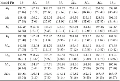
Table 2.5: Means and Standard Errors of AIC Posterior Mean Data Generating Process

M0 134.28 197.15 320.72 191.77 252.44 533.40 354.33 539.01 (7.45) (15.98) (25.63) (12.52) (19.52) (37.62) (29.40) (36.43) Mh 138.41 159.21 325.05 194.40 196.56 537.15 328.54 501.36

(7.28) (7.03) (25.65) (11.99) (13.51) (37.66) (27.55) (34.94) Mt 142.38 205.36 136.21 173.18 236.21 164.62 198.07 239.68

(3.55) (16.13) (8.35) (10.11) (17.13) (12.95) (16.69) (23.50) Mb 136.37 197.93 207.97 157.92 201.64 227.15 193.56 181.33

(7.20) (15.90) (14.08) (6.95) (14.40) (15.65) (11.87) (13.03) Mbh 142.51 163.02 214.79 163.58 165.45 234.12 184.46 174.53

(7.05) (6.75) (14.13) (6.85) (7.12) (15.59) (10.57) (10.42) Mtb 144.21 203.75 137.92 165.81 207.14 151.14 186.13 174.49

(6.91) (15.68) (8.27) (6.92) (14.06) (7.32) (11.74) (12.97) Mth 153.84 174.97 147.71 176.99 181.10 161.94 166.74 165.08

(6.14) (6.44) (7.36) (6.20) (7.45) (7.00) (6.23) (7.90) Mtbh 155.64 176.64 149.40 177.14 179.82 162.12 168.48 163.48

(5.94) (6.30) (7.50) (6.14) (6.16) (6.55) (6.15) (6.57)

where ˆθis the MLE ofθunder the assumed model. However, our AIC calculation is different from the usual form of AIC. Defining

D(θ) =₋2LogL(θ_|X),

we use AIC = E[D(θ)_|X] + 2p0 _where _E[D(θ)

|X] represents the mean of the posterior

distribution of D(θ).

(41)

Table 2.6: AIC Model Selection: Percentage of times each model selected Data Generating Process (DGP)

M0 92 0 0 0 0 0 0 0

Mh 0 95 0 0 0 0 0 0

Mt 1 0 87 0 0 1 0 0

Mb 7 0 0 99 0 0 0 0

Mbh 0 5 0 1 99 0 2 12

Mtb 0 0 13 0 0 98 3 10

Mth 0 0 0 0 1 2 87 36

Mtbh 0 0 0 0 0 0 8 44

Model Selection Error 8 5 13 1 1 2 13 52

matches the data generating assumptions. This suggests that although estimation of N may be biased even in the correct model, the AIC is capable of identifying it correctly.

Perhaps more indicative of the performance of AIC is the summary in Table 2.6, which tells us the percentage of selections for each model using the AIC criterion. Ideally, the diagonal entries in the table should have the highest percentages of selections by AIC. The columns of the table represent the true model generating assumptions. When another model is selected by AIC, this may be called a model selection error, and the percentage of times AIC makes a model selection error is listed in Table 2.6. In this respect, for seven of the eight models, AIC performs quite well as a model selection tool. Among these seven models, for Mt and Mth, the percentage of selections is 87 percent, which is somewhat

lower than for the other models. When Mt and Mth are not selected by AIC, though,

(42)

assumptions ofMtbh only produced a 44 percent selection rate by AIC. WhenMtbh was not

selected in this column, the model selected was one of the sub-models containing two of the effects (Mth, Mbh, and Mtb). Some of this could be due to relative weighting of the time,

behavioral, and heterogeneity effects withinMtbh, as AIC may be picking the model based

on the most significant of these effects present in any particular data set. Furthermore, as previously stated, with five captures, model Mtbh may be somewhat over-parameterized.

We observe 31 distinct capture histories, and model Mtbh includes 13 parameters for such

data, which may lead to the estimation of effects due only to random chance. However, from an overall look at this table, we conclude that AIC performs well as a model selection tool.

2.3.4 Analysis of DIC as a Model Selection Criterion

The DIC criterion is a recent development in model selection. DIC can be ex-pressed in a form similar to AIC. Given the common use of AIC, this feature allows users to quickly understand the form and use of DIC. Another significant benefit of DIC is that it is easy to calculate, as it is just a function of the posterior parameters and the model deviance (where deviance is related to the log-likelihood).

DIC can be expressed similarly to AIC. Using the same notation as in the definition of AIC, and again denoting

D(θ) =₋2LogL(θ_|X),

and defining

(43)

where again E(D(θ)_|X) represents the posterior mean of the deviance function D(θ), we denote

DIC =D(ˆθ) + 2pD (2.2)

where ˆθis a posterior estimate of θ, e.g., ˆθ=E[θ_|X] orM edian[θ_|X]. As stated previously, thepD term in DIC represents an effective number of parameters. The pD term measures the decrease in the deviance (corresponding to increase in the likelihood) obtained by using posterior estimates of the parameters θ. It is important to note that although DIC is structured to look like AIC, the penalty term is actually a function of the fit of the model itself, not simply a discrete number of parameters.

Generally for computational purposes, defining Dev(θ) as the MCMC computed deviance for any particular data set and model combination, and defining ¯Das the MCMC mean of the deviance statistic, pD is computed as

pD= ¯D₋Dev(ˆθ)

and computationally, we have

DIC =Dev(ˆθ) + 2pD.

In our simulations, DIC did not perform as well as AIC in model selection. A table of how often each of the models was selected using the DIC criterion is given in Table 2.8. For simple data sets (such as M0, Mb, or Mt), DIC selects a more complex

(44)

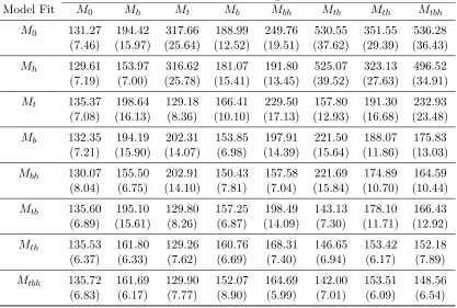
Table 2.7: Means and Standard Errors of DIC Data Generating Process (DGP)

M0 131.26 194.41 317.65 188.98 249.75 530.54 351.55 536.27 (7.46) (15.97) (25.64) (12.52) (19.51) (37.62) (29.39) (36.43) Mh 123.25 152.09 311.45 178.64 191.05 522.87 320.33 494.86

(13.16) (7.47) (26.20) (14.59) (13.22) (38.75) (28.15) (34.75) Mt 135.36 198.64 129.17 166.41 229.50 157.80 191.30 232.92

(7.08) (16.13) (8.36) (10.10) (17.13) (12.93) (16.68) (23.48) Mb 131.75 194.10 201.89 153.23 197.82 221.08 187.70 175.48

(7.28) (15.90) (14.06) (7.13) (14.40) (15.63) (11.86) (13.03) Mbh 100.64 150.71 140.52 127.81 149.81 173.37 162.60 156.78

(16.40) (8.46) (24.48) (14.50) (9.68) (24.84) (20.69) (15.65) Mtb 129.33 182.62 129.50 150.70 186.95 142.88 177.15 165.39

(7.74) (21.30) (8.23) (6.93) (16.50) (7.27) (11.51) (12.70) Mth 120.43 161.64 112.19 155.77 168.23 141.73 153.12 151.97

(17.52) (6.30) (17.98) (8.59) (7.35) (9.49) (5.89) (7.91) Mtbh 126.15 157.44 125.47 145.35 157.55 131.03 151.99 145.74

(13.44) (7.39) (9.33) (8.52) (8.05) (11.40) (5.84) (7.26)

number of selections of modelMbh across all data sets. The problem with DIC arises in the

computation of the penalty term pD. Although pD is positive in most cases, it is possible that pD can be negative for a particular model and data set, if the likelihood function is not log-concave. IfpD is negative, instead of being penalized for the model complexity, the model is in fact rewarded by a negative pDvalue.

In Table 2.9, Mbh and other models have negative meanpDvalues in our

simula-tions. In particular, modelMbh frequently has a negative pD. These negative values cause

Mbh to be selected by DIC a significant number of times, even often in cases where the

(45)

Table 2.8: DIC Model Selection: Percentage of times each model selected Data Generating Process (DGP)

M0 0 0 0 0 0 0 0 0

Mh 1 37 0 0 0 0 0 0

Mt 0 0 2 0 0 0 0 0

Mb 0 0 0 0 0 0 0 0

Mbh 82 51 13 95 78 5 15 13

Mtb 0 1 1 1 2 0 0 0

Mth 14 0 71 1 0 7 38 9

Mtbh 3 11 13 3 20 88 47 78

Model Selection Error 100 73 98 100 22 100 62 22

Table 2.9: mean values of pD: ¯D(θ) - D(ˆθ) Data Generating Process (DGP)

M0 0.97 1.26 0.93 1.22 1.30 1.14 1.22 1.26 Mh -7.16 0.89 -5.60 -7.76 2.49 -6.28 -0.21 1.50

Mt 4.98 5.27 4.96 5.24 5.29 5.18 5.23 5.24

Mb 1.38 2.17 -0.08 1.31 2.18 -0.06 0.14 0.15

Mbh -29.87 -0.31 -62.27 -23.77 -3.64 -48.75 -9.86 -5.75

Mtb -0.88 -7.13 5.58 -1.11 -6.19 5.74 5.02 4.90

Mth -9.40 10.67 -11.52 2.78 11.13 3.79 10.37 10.89

(46)

Table 2.10: Means and Standard Errors of DIC: when posterior median used for ˆθ Data Generating Process

M0 131.27 194.42 317.66 188.99 249.76 530.55 351.55 536.28 (7.46) (15.97) (25.64) (12.52) (19.51) (37.62) (29.39) (36.43) Mh 129.61 153.97 316.62 181.07 191.80 525.07 323.13 496.52

(7.19) (7.00) (25.78) (15.41) (13.45) (39.52) (27.63) (34.91) Mt 135.37 198.64 129.18 166.41 229.50 157.80 191.30 232.93

(7.08) (16.13) (8.36) (10.10) (17.13) (12.93) (16.68) (23.48) Mb 132.35 194.19 202.31 153.85 197.91 221.50 188.07 175.83

(7.21) (15.90) (14.07) (6.98) (14.39) (15.64) (11.86) (13.03) Mbh 130.07 155.50 202.91 150.43 157.58 221.69 174.89 164.59

(8.04) (6.75) (14.10) (7.81) (7.04) (15.84) (10.70) (10.44) Mtb 135.60 195.10 129.80 157.25 198.49 143.13 178.10 166.43

(6.89) (15.61) (8.26) (6.87) (14.09) (7.30) (11.71) (12.92) Mth 135.53 161.80 129.26 160.76 168.31 146.65 153.42 152.18

(6.37) (6.33) (7.62) (6.69) (7.40) (6.94) (6.17) (7.89) Mtbh 135.72 161.69 129.90 152.07 164.69 142.00 153.51 148.56

(6.83) (6.17) (7.77) (8.90) (5.99) (7.01) (6.09) (6.54)

alternative choices for ˆθ could be the posterior median or posterior mode. So, pD can be calculated with these alternatives to the posterior mean of ˆθ. The poor performance of DIC when ˆθ was the posterior mean called for examination of DIC when the posterior median was used for ˆθinstead.

In Tables 2.10, 2.11, and 2.12 the performance of DIC improves when the posterior median is used for ˆθ. However, the model selection error rate is still quite high when compared with that of AIC in Table 2.6. However, in focusing on Tables 2.11 and 2.12, although the meanpDvalues are negative less frequently when using the posterior median, the mean pD value is still negative for the Mh and Mbh models. Secondly, in Table 2.12,

(47)

Table 2.11: mean values of pD: ¯D(θ) - D(ˆθ) where ˆθ is the Posterior Median Data Generating Process

M0 0.99 1.27 0.94 1.23 1.32 1.14 1.23 1.27 Mh -0.81 2.77 -0.43 -5.33 3.24 -4.08 2.59 3.16

Mt 4.99 5.27 4.97 5.24 5.29 5.18 5.23 5.24

Mb 1.98 2.26 0.34 1.94 2.27 0.35 0.51 0.50

Mbh -0.44 4.48 0.12 -1.15 4.13 -0.43 2.43 2.06

Mtb 5.40 5.35 5.88 5.43 5.35 5.99 5.97 5.94

Mth 5.69 10.83 5.55 7.77 11.22 8.71 10.68 11.09

Mtbh 6.08 11.05 6.49 0.93 10.86 5.88 11.03 11.07

Table 2.12: DIC Model Selection: Percentage of times each model selected when posterior medians used for ˆθ

Data Generating Process

M0 8 0 0 0 0 0 0 0

Mh 44 79 0 2 0 0 0 0

Mt 2 0 52 0 0 0 0 0

Mb 1 0 0 10 0 0 0 0

Mbh 40 15 0 55 95 0 0 4

Mtb 3 0 15 0 0 31 0 1

Mth 0 2 25 1 1 17 71 21

Mtbh 2 4 8 32 4 52 29 74

(48)

was generated under the assumptions of model Mt, DIC chose modelMt for 52 of the 100

data sets. Alternative models chosen for the other 48 data sets were Mtb, Mth, andMtbh,

which are more complex versions of modelMt. Although all the chosen models account for

time effects, they also contain effects such as behavioral effects and heterogeneity effects that were not present in the population. DIC also selects a more complex model than necessary for data generated under models Mb and Mh. Overall, though, the performance

of DIC in model selection for these models is inferior to that of AIC, and based on this simulation study, use of AIC as a model selection tool is recommended over DIC.

2.4 Further Simulation Experiments

To determine whether our conclusions reached in Section 2.3 hold in general, we examined whether our conclusions held under data generated with the following factors:

1. True Population SizeN

2. Amount of Heterogeneity in the Data (Small Amount, Large Amount)

3. Magnitude of Time Effects

4. Direction of Behavioral Effects

5. Average Capture Probability

(49)

Experiment N Averagepij Time Effects Behavioral Effects Heterogeneity

1 500 0.2 Large Positive Large

2 500 0.2 Small Positive Small

3 500 0.4 Large Negative Large

4 100 0.4 Large Positive Small

5 100 0.4 Small Positive Large

6 100 0.2 Large Negative Small

7 500 0.4 Small Negative Small

8 100 0.2 Small Negative Large

Table 2.13: Data generating assumptions for simulation experiments 1 to 8

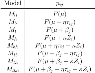
Model pij

M0 F(µ)

Mb F(µ+ητij)

Mt F(µ+βj)

Mh F(µ+κZi)

Mbh F(µ+ητij +κZi)

Mtb F(µ+βj+ητij)

Mth F(µ+βj+κZi)

Mtbh F(µ+βj+ητij +κZi)

Table 2.14: Calculations of pij for simulation experiments 1 to 8; F refers to the Logistic

distribution function F(x) = [1 +e−x_]−1 , Zi i

.i.d.

∼ N(0,1), τij = 1 if the animal has been

previously captured, andτij = 0 otherwise; values ofµ, η, φj,and κ are given in Table 2.15

to a Fractional Factorial experimental design, with the goal of performing a total of eight analyses (including the one described in Section 2.3). Our method of data generation follows the same process as that outlined in Table 2.2, but is described in more detail in Tables 2.13 - 2.15.

For experiments two through eight, we analyzed a total of fifty data sets generated under each model’s assumptions. That is, we generated fifty data sets with constant capture probability (Model M0), fifty with time effects (Model Mt), etc. Because there are eight

(50)

Experiment µ φj η κ

1 F−1_{(0.2) = -1.385} j−3

2 forj= 1, ...,5 +1 1.25 2 -1.385 j−₄3 forj= 1, ...,5 +1 0.25 3 F−1_{(0.4) = -0.405} j−3

2 forj= 1, ...,5 -1 1.25 4 -0.405 j−₂3 forj= 1, ...,5 +1 1.25 5 -0.405 j−₄3 forj= 1, ...,5 +1 0.25 6 -1.385 j−₂3 forj= 1, ...,5 -1 1.25 7 -0.405 j−₄3 forj= 1, ...,5 -1 0.25 8 -1.385 j−₄3 forj= 1, ...,5 -1 0.25

Table 2.15: Design specifications for simulation experiments 1 to 8

capture probabilitiespij for all simulation experiments are listed in Table 2.16. Results of

simulation experiments two through eight are displayed in Figures 2.1 through 2.7. Recall that the primary observations from the first experiment were:

1. Models with behavioral effects, but not time effects, provide a poor estimate ofN, on average, for data sets with time effects present.

2. Population sizes for data sets with a small number of effects (such as those generated under the assumptions of M0, Mb, or Mt) can be accurately estimated, on average,

when the correct model is selected.

3. Heterogeneity in the population leads to negatively biased estimates of population size, even when the correct model is fit.

4. AIC selects the correct model a large percentage of the time.

(51)

Experiment M0 Mb Mt Mh Mtb Mbh Mth Mtbh

1 0.2 0.27 0.39 0.25 0.28 0.28 0.27 0.32 (0) (0.10) (0.27) (0.20) (0.18) (0.22) (0.22) (0.28) 2 0.2 0.27 0.22 0.20 0.27 0.27 0.21 0.27

(0) (0.10) (0.12) (0.04) (0.14) (0.11) (0.07) (0.15) 3 0.4 0.29 0.41 0.42 0.31 0.33 0.43 0.34

(0) (0.10) (0.16) (0.24) (0.12) (0.21) (0.26) (0.22) 4 0.4 0.53 0.41 0.40 0.50 0.53 0.41 0.50

(0) (0.12) (0.16) (0.06) (0.24) (0.14) (0.17) (0.24) 5 0.4 0.53 0.40 0.42 0.52 0.52 0.43 0.50

(0) (0.12) (0.08) (0.24) (0.18) (0.28) (0.24) (0.29) 6 0.2 0.16 0.22 0.20 0.18 0.16 0.22 0.18

(0) (0.05) (0.11) (0.04) (0.10) (0.06) (0.12) (0.10) 7 0.4 0.29 0.40 0.40 0.30 0.29 0.40 0.30

(0) (0.10) (0.08) (0.06) (0.08) (0.11) (0.10) (0.09) 8 0.2 0.16 0.21 0.26 0.17 0.19 0.26 0.20

(0) (0.05) (0.06) (0.20) (0.06) (0.16) (0.21) (0.16)

(52)

For simulation experiments two through eight, DIC continued to perform poorly as a model selection tool. This is again due to the occurrence of negative penalty termspD. For this reason, the results of DIC for simulation experiments two to eight are omitted.

Figures 2.1 through 2.7 give results for both the average MCMC posterior median ofN, and the AIC selection percentages, for the fifty data sets generated under each model’s assumptions. Tables of the average posterior medians of N, and the average values of AIC are given in Section 2.6.

2.4.1 Simulation Experiment Two Summary

In the top panel of Figure 2.1, the horizontal axis is the true model used to generate the data. The vertical axis is the average value of the MCMC posterior median of N for the fifty data sets generated under the assumed model. Finally, because each data set was fitted under each of the eight models, there are eight separate plotted points, one for each model fit, for each data generating model. The posterior median ofN for each fitted model is plotted according to symbols in the legend box at the right of the graph.

The bottom panel in Figure 2.1 gives AIC selection percentages for all the data sets generated for experiment two. The horizontal axis of this graph is the same as in the top panel of Figure 2.1. The vertical axis is the percentage of AIC selections out of the fifty data sets generated for each model. The bar shading indicates which fitted model (from the shading described in the legend box) is selected. The bars are stacked so that their total is one-hundred percent for each of the models.

(53)

Figure 2.1: Experiment 2 Posterior Median and AIC Results (TrueN = 500) Posterior Median of N, Run 2

250 500 750 1000

M0 Mb Mt Mh Mtb Mbh Mth Mtbh

DGP A vg P os te ri or M ed ia n of N _M0 Mb Mt Mh Mtb Mbh Mth Mtbh

AIC Selection Rates, Run 2

0% 20% 40% 60% 80% 100% 120%

DGP A IC S el ec tio n R at e

Mtbh

Mth

Mbh

Mtb

Mh

Mt

Mb

M0

fit to theMb data split into two groups. In the picture, modelsM0, Mt, Mh, andMth show

negative bias. Models with behavioral effects (Mb, Mtb, Mtbh have average posterior median

values close to 500, ranging between 475 to 525). Model Mbh shows bias in estimating N,

(54)

N when fit to data generated under Model Mt assumptions (because the time effects in

experiment two are small in magnitude). However, as in the first simulation experiment, modelsMb andMbhare significantly positively biased when fitting data with time effects but

not behavioral effects. The data sets generated under ModelMh show that all eight models

show small to negligible bias in estimating N, due to the small heterogeneity effect in the data sets (see Table 2.13). When the amount of heterogeneity is small, the data sets come close to having a constant capture probability, and all eight models estimate N accurately when capture probabilities are constant. Model Mtb data shows that Model Mtb has the

smallest bias in estimating N , which is expected. ModelsMb, Mtb,and Mbh show at most

small biases for estimatingN when the data are from ModelMbh. All three of these models

account for the behavior effects in the data. Model Mth data showed accurate estimation

of N by all models except Mb and Mbh, because both the time effects and heterogeneity

effects are small in magnitude, so most models are appropriate for these data sets, except for those with behavior effects and not time effects. Lastly, data sets generated with all three effects (time, behavior, and heterogeneity) haveN estimated best by Models Mtb and

Mtbh, although negative bias is seen in the estimates ofN of these models.

The AIC results are favorable for data generated under models M0, Mb, Mt and

Mtb. We note from Figure 2.1 that AIC selects Model M0 regularly for the Mh data sets.

(55)

Mtbh data, AIC selects Model Mtb most often. For Mth data, Model Mtis most commonly

selected. It appears that the smaller magnitude of the heterogeneity effect for these data sets means that a heterogeneity effect in the model is not necessary to provide adequate fit to the data.

2.4.2 Experiment Three Summary

In Figure 2.2, all eight models have small, if any, bias in estimatingN for the Model M0data sets, as all the average posterior medians ofNare close to the trueN = 500. For the Mb data sets, the Models Mb, Mtb, Mbh andMtbh have posterior medians close toN = 500,

while the other model estimates are positively biased, because the behavioral effect for the experiment three data is negative, and models without behavioral effects overestimate N. For theMt data sets, most models accurately estimate N, except for ModelsMb and Mbh,

which are significantly positively biased, matching the results from experiment one. For the Mh data sets, the most accurate estimation of N occurs for a cluster of models including

Mh,Mth,Mbh, and Mtbh, all of which show negative relative bias in estimatingN of about

seven percent. Of these four models, Model Mbh has the smallest absolute bias. This is

similar to the results of experiment one, when the heterogeneity in the data was also large. Analysis of the Mtb data sets showed that the most accurate estimates of N occurred for

Models Mtb and Mtbh, which both have average posterior median close to N = 500, with

Model Mtb having the smallest relative bias, which is positive and near two percent. For

the Mbh data sets, the best estimates of N are given by Models M0, Mt, Mtb, and Mtbh.

The Model Mbh posterior median is below the true N = 500, with a negative relative bias

(56)

250 500 750 1000

DGP A vg P os t. M ed ia n of N M0 Mb Mt Mh Mtb Mbh Mth Mtbh

0% 20% 40% 60% 80% 100% 120%

Mtbh

Mth

Mbh

Mtb

Mh

Mt

Mb

M0

bias in estimating N, matching the results from simulation experiment one. For the Mth

data sets, the cluster of models Mh, Mtb, Mth and Mtbh are closest to the true N = 500,

but all show negative relative bias of between three and seven percent. For the Mtbh data

(57)

five-hundred. The modelsMhand Mth have averages above but close to the trueN = 500. The

other models mentioned show small negative bias in estimating N. Again, the behavioral modelsMb andMbh show large positive biases in estimating N.

The AIC analysis in Figure 2.2 shows that for the data sets in experiment three, AIC selects the true model the majority of the time for all data sets. This is due to the combination of the strong heterogeneity effects, large time effects, and large population size N = 500. AIC tells us that these data sets, given the strong underlying effects mentioned, are best fit by models that account for all the underlying sources of variability in capture probabilities.

2.4.3 Experiment Four Summary

Figure 2.3 gives results for simulation experiment four. In the first graph, all the points are very tightly clustered around the true value ofN = 100, except when time effects are present in the data, and the model fit has behavior effects but not time effects. This tight clustering of the model results occurs because the average capture probability is high (near 40%) and the heterogeneity effects are small. Although the time effects are significant, because the average capture probability is high, even models which do not account for them, such asM0, still provide an adequate fit, in the sense that on average, the posterior median of N is close to one-hundred.

Analysis of Figure 2.3 for the AIC results gives similar conclusions to those in experiment two. That is, M0, Mb, Mt, and Mtb data sets are selected most often by their

(58)

0 100 200 300

DGP A vg . P os te ri or M ed ia n of N _M0 Mb Mt Mh Mtb Mbh Mth Mtbh

0% 20% 40% 60% 80% 100% 120%

Mtbh

Mth

Mbh

Mtb

Mh

Mt

Mb

M0

effects. It is noted, though, that the data sets generated under ModelMtbhdo not specifically

(59)

2.4.4 Experiment Five Summary

60 80 100 120 140 160

DGP A vg P os te ri or M ed ia n of N _M0 Mb Mt Mh Mtb Mbh Mth Mtbh

0% 20% 40% 60% 80% 100% 120%

DGP A IC S el ec tio n R at e Mtbh Mth Mbh Mtb Mh Mt Mb M0

In Figure 2.4, the M0 data sets are fit well by most models, with the highest observed relative bias in the posterior median ofN being about 10%, for the ModelMtb fit.

For the Mb data sets, the models Mb and Mtbh show negligible bias in estimating N, with