A modified scout bee for artificial bee colony algorithm and its performance on optimization problems

(1)

A modified scout bee for artificial bee colony

algorithm and its performance on optimization

problems

Syahid Anuar

a

, Ali Selamat

a,b,*

_{, Roselina Sallehuddin}

a

Faculty of Computing, Universiti Teknologi Malaysia, Malaysia b

UTM-IRDA Digital Media Center of Excellence, Universiti Teknologi Malaysia, Malaysia

Received 27 June 2015; revised 12 March 2016; accepted 13 March 2016 Available online 23 April 2016

KEYWORDS

Artiﬁcial bee colony algo-rithm;

Optimization; Swarm intelligence

Abstract The artiﬁcial bee colony (ABC) is one of the swarm intelligence algorithms used to solve

optimization problems which is inspired by the foraging behaviour of the honey bees. In this paper, artiﬁcial bee colony with the rate of change technique which models the behaviour of scout bee to improve the performance of the standard ABC in terms of exploration is introduced. The technique is called artiﬁcial bee colony rate of change (ABC-ROC) because the scout bee process depends on the rate of change on the performance graph, replace the parameterlimit. The performance of ABC-ROC is analysed on a set of benchmark problems and also on the effect of the parametercolony size. Furthermore, the performance of ABC-ROC is compared with the state of the art algorithms.

Ó2016 King Saud University. Production and hosting by Elsevier B.V. This is an open access article under

the CC BY-NC-ND license (http://creativecommons.org/licenses/by-nc-nd/4.0/).

1. Introduction

The ABC algorithm is introduced byKaraboga (2005), based

on the foraging behaviour of a honey bees swarm. In ABC, the

colony of artiﬁcial bees consists of three groups namely employed, onlooker and scout. A food source position repre-sents a possible solution to the problem that is to be optimized and the nectar of a food source corresponds to the quality of the solution represented by the food source. During each cycle, the employed and onlooker bees are moving toward the food sources, thus calculating the nectar amounts and determining the scout bee and then moving them randomly onto the possi-ble food sources. If the solution does not improve by a prede-termined number of trials, the food source is abandoned. The number of trials for releasing a food source is equal to the

value of limit which is an important control parameter of

ABC (Karaboga and Gorkemli, 2014). After the limit is

achieved, the employed bee is converted to a scout to search for new food sources.

The scout bee is an important component to control the

exploration process (Karaboga and Basturk, 2008). However,

* Corresponding author at: Faculty of Computing, Universiti Teknologi Malaysia, Malaysia. Tel.: +60 7 5532222, +60 7 5538009; fax: +60 7 5565044. He is also a visiting professor at University of Hradec Kralove, FIM, Center for Basic and Applied Research, Rokitanskeho, 62, Hradec 9 Kralove, 500 03, Czech Republic.

E-mail address:aselamat@utm.my(A. Selamat).

Peer review under responsibility of King Saud University.

Production and hosting by Elsevier

King Saud University

Journal of King Saud University –

Computer and Information Sciences

www.ksu.edu.sa www.sciencedirect.com

http://dx.doi.org/10.1016/j.jksuci.2016.03.001

1319-1578Ó2016 King Saud University. Production and hosting by Elsevier B.V.

(2)

recent studies on ABC show that the scout bee component is redundant and sometimes does not present during the search

process (Bullinaria and AlYahya, 2014a,b). As a result, the

global exploration does not happen during the process because the global exploration is controlled by the scout bee

compo-nent (Karaboga and Basturk, 2007). Therefore, we propose a

new technique to control the scout bee process.

In this study, we propose a technique to replace thelimitof

the standard ABC algorithm. This technique is based on the changing of slope on the performance graph. The optimization process causes a decrease in the performance graph in case of function minimization and increasing of the performance graph in case of function maximization until the stopping con-dition achieved. By taking advantage of the changing pattern on the performance graph, we introduce a new technique called rate of change (ROC) to improve the performance of ABC in terms of exploration. The implementation of ROC technique in ABC algorithm is called artiﬁcial bee colony rate of change (ABC-ROC). Later, the ABC-ROC will be described in detail and its performance is tested on a set of test problems. The effect of newly added control parameters such as max-ROC, maxTrace and maxFlag is investigated. The perfor-mance of ABC-ROC is also compared to the state of the art algorithms.

The rest of this paper is organized as follows. Section2

dis-cusses the literature review on ABC. Section 3 provides an

overview of ABC algorithm. Section4describes the proposed,

ABC-ROC algorithm. Section5gives a computational study

and discussion, that include the explanation of the problems

used in this experiment. Section 6 presents the experimental

complexity of ABC and ABC-ROC algorithms. Section7

pre-sents the experiment on the effect of colony size (CS). Section8

presents the comparisons of the number of scout bee between

ABC and ABC-ROC. Finally, Section9concludes this paper

and suggests the future direction.

2. Literature review

The standard ABC algorithm has successfully produced good results in the optimization problem because ABC has advan-tages of memory, local search and solution improvement

mechanism (Basturk and Karaboga, 2006; Karaboga and

Basturk, 2007, 2008; Zhao et al., 2010; Ozturk and Karaboga, 2011). However, in some cases, researchers found ABC may stuck in local optimum that affects the convergence performance and resulted in uncertainties on the results

obtained from the standard ABC algorithm (Luo et al.,

2013; Xiang and An, 2013; Kong et al., 2013).

Some researchers argued that the problem arose from the exploration process while other researchers believed that the problems are caused by the exploitation process of ABC. The exploration is the ability to investigate the various unknown region to discover the global optimum in solution space. This ability is performed by the scout bee component (Kong et al., 2013; Karaboga and Basturk, 2007). The exploitation is the ability to apply the knowledge of the previ-ous good solutions to ﬁnd better solutions. This process done

by employed and onlooker bees (Kong et al., 2013; Karaboga

and Basturk, 2007). In order to improve the exploration and exploitation process, many changes have been made on the standard ABC algorithm.

Aderhold et al. investigated the influence of the population size of the ABC and proposed two variants of ABC which use new methods for the position update of artificial bees (Aderhold et al., 2010). Stanarevic et al. proposed a modified

ABC which includes ‘‘smart bee”that uses its historical

mem-ories of location and quality of the food source (Stanarevic

et al., 2010). Lei et al, discovered that original ABC suffers from low precision and efﬁciency in solving optimization prob-lems thus introduced a modiﬁcation of the original ABC by adding an inertial weight which was inspired by particle swarm

optimization (Lei et al., 2010).

Funcon evaluaon (FE)

Fu

nc

on

v

al

ue

S

inial

S

ﬁnal

Figure 1 Illustration of slope in graph.

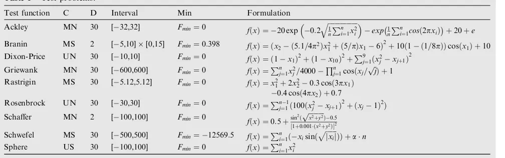
Table 1 Test problems.

Test function C D Interval Min Formulation

Ackley MN 30 [32,32] Fmin¼0 _f_ð_x_{Þ ¼}_{20 exp} ₀_:₂ ffiffiffiffiffiffiffiffiffiffiffiffiffiffiffiffiffiffi1

n Pn

i¼1x2i

q

exp1

n Pn

i¼1cosð2pxiÞ

_þ

20þe

Branin MS 2 [5,10][0,15] Fmin¼0:398 _fð_xÞ ¼ ð_x₂ ð5_:1₌4p2_Þ_x2

1þ ð5=pÞx16Þ 2

þ10ð1 ð1₌8pÞÞcosðx1Þ þ10

Dixon-Price UN 30 [10,10] Fmin¼0 fðxÞ ¼ ð1x1Þ2þ ð1x10Þ2þP9j¼1ðx2jxjþ1Þ

2

Griewank MN 30 [600,600] Fmin¼0 fðxÞ ¼Pnj¼1x2j=4000

Qn

j¼1cosðxj= ﬃﬃj

p

Þ þ1

Rastrigin MS 30 [5.12,5.12] Fmin¼0 fðxÞ ¼x12þ2x220:3 cosð3px1Þ

0:4 cosð4px2Þ þ0:7

Rosenbrock UN 30 [30,30] Fmin¼0 fðxÞ ¼Pn1

j¼1ð100ðx2jxjþ1Þ

2

þ ðxj1Þ2Þ

Schaffer MN 2 [100,100] Fmin¼0 _f_ð_x_{Þ ¼}₀_:₅_þsin2_ðpffiffiffiffiffiffiffiffiffiffi_x2þy2Þ0:5

½1þ0:001ðx2_þ_y2_Þ2

Schwefel MS 30 [500,500] Fmin¼ 12569:5 fðxÞ ¼Pn_i_¼₁ðxisinð

ffiffiffiffiffiffiffi jxij p

ÞÞ þan

(3)

Lee and Cai proposed a new diversity strategy to balance

the exploration and exploitation of ABC algorithm (Lee and

Cai, 2011). Further, Zou et al. introduced a new variant of the ABC algorithm based on Von Neumann topology (VABC)

and evaluated the performance on clustering problem (Zou

et al., 2011). Stanarevic studied the new approach of mutation strategies of the standard ABC by implementing ﬁve different types of mutation strategies adapted from differential evolu-tion algorithm in order to improve the exploitaevolu-tion

perfor-mance of ABC (Stanarevic, 2011).

Akay and Karaboga proposed a modiﬁed ABC by control-ling the frequency of perturbation to improve the convergence

rate (Akay and Karaboga, 2012). Yan et al. proposed a hybrid

ABC (HABC) by introducing the crossover operator of genetic algorithm (GA) to enhance the information exchange between

bees (Yan et al., 2012). Moreover, Kashan et al introduced a

new version of ABC called DisABC which was designed for

binary optimization (Kashan et al., 2012).

Kong et al. proposed an improved ABC called IABC to balance the exploration and exploitation of the standard ABC by employing the orthogonal initialization method (Kong et al., 2013). Xiang et al. proposed an efﬁcient and robust artiﬁcial bee colony (ERABC) by employing chaotic search on scout bee phase and combinatorial solution search

equation to accelerate the search process (Xiang and An,

2013). Luo et al. implemented a modiﬁcation on the onlookers

bee of ABC and called the modiﬁed algorithm as convergence-onlookers ABC (COABC) in order to improve the exploitation (Luo et al., 2013).

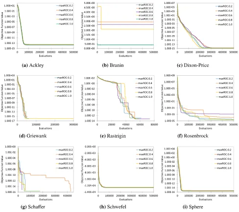
Figure 2 Convergence performance on various numerical functions for differencemaxROCvalues.

Table 2 Parameters setting for ABC-ROC.

Related parameter Test parameter

maxROC maxTrace maxFlag

maxROC – 0.5 0.5

maxTrace 10 – 10

(4)

Karaboga and Gorkemli introduced a new version of ABC that model the behaviour of onlooker bee more accurately to improve the local search ability. The improvement is called

quick ABC or qABC (Karaboga and Gorkemli, 2014).

Han-bay and Talu proposed an improved artiﬁcial bee colony (I-ABC) to search for the optimal threshold value of synthetic

aperture radar (SAR) image (Hanbay and Talu, 2014). Maeda

and Tsuda presented a reduction of artiﬁcial bee colony algo-rithm which reduced the number of bees sequentially to reach a

predetermined value (Maeda and Tsuda, 2015).

Kiran and Findik added a directional information to ABC algorithm for each design parameter in order to cope with the

slow convergence performance of the standard ABC (Kran

and Fndk, 2015). Ozturk et al. proposed a new solution gener-ation mechanism for the discrete version of ABC using all sim-ilarity cases through the genetically inspired components (Ozturk et al., 2015).

In this paper, we consider to control the process of scout bee by introducing ROC technique. The ROC technique is considered the changing of slope on the performance graph.

This technique is able to monitor the presence of local opti-mum on the graph itself. The proposed ROC technique is tested on numerical benchmark functions.

3. Artificial bee colony algorithm

The ABC model consists of three groups of bees which are employed, onlooker and scout that differ in terms of their functionality. Employed bee go to the food sources and come back to hive and exchange the information with onlooker bee by dancing on the dance area. Onlooker bee watches the dances and chooses the food sources depending on the dance moves. The employed bee which food sources have been aban-doned becomes a scout and starts searching for a new food source.

For the purpose of optimization, the position of the food source represents a possible solution to the optimization prob-lem and the nectar amount of a food source corresponds to the quality (ﬁtness) of the associated solution. The number of employed or onlooker is equal to the number of solutions in

Table 3 Comparisons of different setting of parameter maxROC.

Problem Statistic Parameter

maxROC:0.2 maxROC:0.4 maxROC:0.6 maxROC:0.8 maxROC:1.0

Ackley Mean 3.52E14 3.49E14 3.51E14 3.45E14 3.53E14

SD 4.51E15 3.92E15 5.07E15 3.82E15 4.58E15

Best 2.93E14 2.93E14 2.22E14 2.93E14 2.22E14

Worst 4.35E14 4.00E14 4.35E14 4.00E14 4.00E14

Branin Mean 3.98E01 7.57E+00 5.68E+00 5.72E+00 3.98E01

SD 0.00E+00 3.33E+00 2.15E+00 2.25E+00 0.00E+00

Best 3.98E01 2.92E+00 2.64E+00 2.12E+00 3.98E01

Worst 3.98E01 1.40E+01 1.10E+01 1.10E+01 3.98E01

Dixon Mean 2.65E15 2.94E15 2.83E15 2.85E15 2.82E15

SD 5.37E16 9.62E16 5.80E16 7.29E16 5.58E16

Best 1.55E15 1.66E15 1.64E15 1.78E15 1.63E15

Worst 3.64E15 6.96E15 4.31E15 5.00E15 4.29E15

Griewank Mean 5.27E12 2.47E04 3.29E04 8.51E17 1.35E04

SD 2.89E11 1.35E03 1.80E03 1.04E16 7.39E04

Best 0.00E+00 0.00E+00 0.00E+00 0.00E+00 0.00E+00

Worst 1.58E10 7.40E03 9.86E03 5.55E16 4.05E03

Rosenbrock Mean 9.50E02 5.70E02 1.66E01 1.68E01 1.39E01

SD 1.41E01 9.97E02 3.04E01 3.02E01 2.99E01

Best 2.46E05 1.19E04 1.22E03 2.27E05 2.01E05

Worst 5.74E01 4.14E01 1.23E+00 1.16E+00 1.55E+00

Schaﬀer Mean 3.05E05 1.90E05 6.66E06 9.27E07 1.23E05

SD 8.71E05 5.90E05 2.54E05 4.80E06 6.74E05

Best 0.00E+00 0.00E+00 0.00E+00 0.00E+00 0.00E+00

Worst 3.33E04 2.79E04 1.02E04 2.63E05 3.69E04

Schwefel Mean 1.26E+04 1.26E+04 1.26E+04 1.26E+04 1.26E+04

SD 1.85E12 1.85E12 1.94E12 1.85E12 1.85E12

Best 1.26E+04 1.26E+04 1.26E+04 1.26E+04 1.26E+04

Worst 1.26E+04 1.26E+04 1.26E+04 1.26E+04 1.26E+04

Sphere Mean 5.20E16 5.36E16 5.51E16 5.18E16 5.34E16

SD 1.07E16 6.77E17 8.32E17 7.83E17 1.14E16

Best 3.19E16 4.61E16 4.22E16 3.16E16 3.15E16

Worst 7.02E16 7.26E16 7.21E16 7.11E16 7.66E16

(5)

the population. For the ﬁrst step, the ABC generates a

ran-domly distributed initial populationP(C= 0) ofSNsolutions

(food source positions), where SN represents the size of

employed or onlooker. Each solutionxiði¼1;2;. . .;SNÞis a

D-dimensional vector where D is the number of parameters

to be optimized. The population of the positions (search pro-cess of the employed, onlooker and scout) is repeated until

the maximum cycle number (MCN), C¼1;2;. . .MCN is

reached.

An employed bee produces a modiﬁcation on the position

using Eq. (1). If the nectar amount of the new position is

higher than before, the bee memorizes the new position and discards the old one. Otherwise, the bee keeps the position of the previous in memory

vij¼xijþ ;ijðxijxkjÞ; ð1Þ

where k2 f1;2;. . .;SNg and j2 f1;2;. . .;Dg are randomly

chosen indexes; k is determined randomly and should

differ fromi, and;ijis a randomly generated number between

[1,1].

After all employed bees complete the search process, the sharing information begins where the food sources and their position information are shared with the onlooker bee. An onlooker bee evaluates the nectar information and chooses a

food source with a probability,p_i, related to its nectar amount

following Eq.(2):

pi¼ fit_i

PSN

n¼1fitn

; ð2Þ

wherefiti is the ﬁtness value of the solution iandSN is the

number of food sources. The employed bee produces a modi-ﬁcation of the position and checks the nectar amount of the candidate source. If the nectar is higher than the previous one, the onlooker bee memorizes the new position and discards the old one.

The food source of which the nectar is abandoned by the bees is replaced with a new food source by the scouts by Eq.

(3) in case the position cannot be improved further. The

parameter ‘‘limit”is the control parameter to determine the

abandonment of the food sources within the predetermined number of cycles

xij¼x j

minþrandð0;1Þðx

j

maxx

j

minÞ: ð3Þ

The main steps of ABC are given as below (Karaboga, 2005):

Step 1:Initialize the population of solutionsxi; i¼1. . .SN

Step 2:Evaluate the population Step 3:cycle = 1

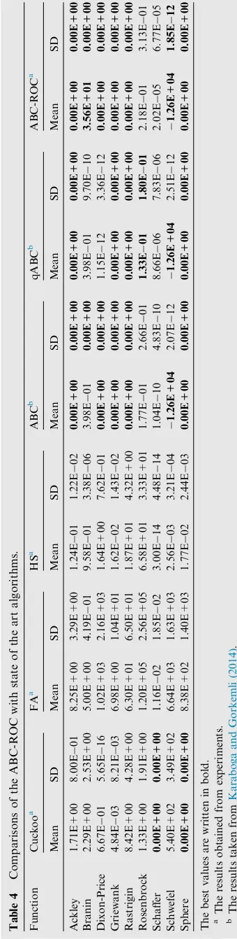
Table 4 Comparisons of the ABC-ROC with state of the art algorithms. Function Cuc koo a FA a HS a AB C b qABC b AB C-ROC a Mean SD Mean SD Mean SD M ean SD Mean SD Mean SD Ackley 1.71E+ 00 8.00E 01 8.25E+ 00 3.29E+ 00 1.24E 01 1.22E 02 0.00E +00 0.00E +00 0.00E+ 00 0.00E+ 00 0.00E+ 00 0.00E+ 00 Branin 2.29E+ 00 2.53E +00 5.00E+ 00 4.19E 01 9.58E 01 3.38E 06 3.98E 01 0.00E +00 3.98E 01 9.70E 10 3.56E+ 01 0.00E+ 00 Dixon-Price 6.67E 01 5.65E 16 1.02E+ 03 2.16E+ 03 1.64E+ 00 7.62E 01 0.00E +00 0.00E +00 1.15E 12 3.36E 12 0.00E+ 00 0.00E+ 00 Griewan k 4.84E 03 8.21E 03 6.98E+ 00 1.04E+ 01 1.62E 02 1.43E 02 0.00E +00 0.00E +00 0.00E+ 00 0.00E+ 00 0.00E+ 00 0.00E+ 00 Rastrig in 8.42E+ 00 4.28E +00 6.30E+ 01 6.50E+ 01 1.87E+ 01 4.32E+ 00 0.00E +00 0.00E +00 0.00E+ 00 0.00E+ 00 0.00E+ 00 0.00E+ 00 Rosenbr ock 1.33E+ 00 1.91E +00 1.20E+ 05 2.56E+ 05 6.58E+ 01 3.33E+ 01 1.77E 01 2.66E 01 1.33E 01 1.80E 01 2.18E 01 3.13E 01 Schaﬀer 0.00E+ 00 0.00E +00 1.16E 02 1.85E 02 3.00E 14 4.48E 14 1.04E 10 4.83E 10 8.66E 06 7.83E 06 2.02E 05 6.77E 05 Schwef el 5.40E+ 02 3.49E +02 6.64E+ 03 1.63E+ 03 2.56E 03 3.21E 04 1.26E +04 2.07E 12 1.26E+ 04 2.51E 12 1.26E+ 04 1.85E 12 Sphere 0.00E+ 00 0.00E +00 8.38E+ 02 1.40E+ 03 1.77E 02 2.44E 03 0.00E +00 0.00E +00 0.00E+ 00 0.00E+ 00 0.00E+ 00 0.00E+ 00 Th e b es t valu es are writ ten in bold. a Th e resu lts obt ained from exper iments. b Th e resu lts take n fr o m Karab oga and Gork emli (2014 ) .

Table 5 Wilcoxon signed rank test results.

Function Mean diﬀerence p-Value

Ackley 3.50E14 0.004

Branin 3.52E+01 0.000

Dixon-Price 2.79E15 0.023

Griewank 0.00E+00 –

Rastrigin 0.00E+00 –

Rosenbrock 4.10E02 0.072

Schaﬀer 2.02E05 0.010

Schwefel 0.00E+00 –

(6)

Step 4:Repeat

Step 5:Produce new solutionvi for the employed bees by

using Eq.(1)and evaluate them

Step 6:Apply greedy selection process. If the solution does not improve, increase the trial counter.

Step 7:Calculate the probability valuespifor the solutions

xiby Eq.(2)

Step 8:Produce the new solutionsvifor the onlookers from

the solutions

Step 9:xi selected depending onpi and evaluate them

Step 10:Apply greedy selection process. If the solution does not improve, increase the trial counter.

Step 11:Determine the abandoned solution for the scout, if

exist (trialPlimit), and replace it with a new randomly

produce solutionxi by Eq.(3)

Step 12:Memorize the best solution achieved so far Step 13:cycle = cycle + 1

Step 14:until cycle = MCN

Based on the procedure of ABC, the scout bee will be

exe-cuted if the ‘‘trial”exceeded the ‘‘limit”. The ‘‘trial”counter

will increase if the solution does not improve and will be reset to zero if the solution is improved during the process of employed and onlooker bees. The employed and onlooker bees will produce local solutions. The local solutions usually will improve but not necessary become the best solution. The best solution is the global solution which will be selected after the employed, onlooker and scout bee process (for example in Step

12). For certain problems such as studied byBullinaria and

AlYahya (2014b), the local solutions are constantly improved, resulting the trial is always reset to zero. Thus, the trial counter does not exceed the limit causing the global exploration by scout bee is difﬁcult to occur. For this reason, an improved scout bee process is proposed. The proposed artiﬁcial bee col-ony rate of change (ABC-ROC) will consider global solution instead of local solution by using slope on graph as reference. The next section will discuss the proposed ABC-ROC.

4. The proposed artificial bee colony rate of change (ABC-ROC)

The scout bee is important to control the exploration process.

The scout bee component is controlled by limit in original

ABC. However, if thelimitdoes not achieve, the scout bee is

not involved in the process. We introduce another technique to control the scout bee process. By taking advantage of the slope on the performance graph, we calculate the slope and keep track the function value. In other words, the process is basically keeping track the rate of change of the performance graph. Thus, we called our proposed technique as rate of change (ROC) technique. Implementation of ROC in ABC algorithm is called artiﬁcial bee colony rate of change (ABC-ROC).

In ABC-ROC, we add three new parameters called

max-Trace,maxROC, andmaxFlag. The maxTrace value decides

the starting point to calculate the slope. In other words,

max-Tracecan be viewed as the straight line on the graph. The

max-ROC value gives a maximum value of the slope to be

considered before calling scout bee. The flagvalue is to keep

track when the graph does not improve orslope¼0.

During the ﬁrst cycle, the initial function value, Sinitial, is

stored in a memory. A counter, (called trace) increases by

one during each cycle. When trace is equal to ‘‘maxTrace”,

the ﬁnal function value is stored as Sfinal andtrace are reset

to zero. Then, the slope is calculated using Eq.(4)

slope

j j ¼dy

dx¼

ðSfinalSinitialÞ

Sinitial

: ð4Þ

Based on Eq.(4), in order to calculate slope, an initial point

and a ﬁnal point are needed. TheSinitialis referred as an initial

point because the initial function value is always higher (in

case of function minimization). Once the ‘‘maxTrace” is

achieved, the ﬁnal point,Sfinal is stored.Fig. 1illustrates the

example of slope in graph.

The advantage of using slope is that it can determine the sit-uation when the solution does not improve (in case of stagna-tion or stuck in local optimum) directly from the graph. The pseudo-code of the proposed ABC-ROC is given below:

Step 1: Set parameters (MCN,SN,maxROC,maxTrace, maxFlag)

Step 2: Initialize the population of solutions

xi; i¼1;2;. . .;SN

Step 3:Evaluate the population

Step 4:cycle = 1; counter = 1; ﬂag = 0; Step 5:repeat

Step 6:Produce new solutionvifor the employed bees using

Eq.(1)and evaluate them

Step 7:Apply the greedy selection process for the employed bees

Step 8:Calculate the probability valuesPifor the solutions

xi using Eq.(2)

Step 9:Produce the new solutionsvifor the onlookers from

the solutionsxiselected depending onPiand evaluate them

Step 10: Apply the greedy selection process for the onlookers

Step 11:if trace ==maxTrace Step 12:Calculate slope using Eq.(4) if slope == 0

Scout bee produce new random solutionxiusing Eq.(3)

ﬂag = ﬂag + 1

maxTrace=maxTrace2

else if slope6maxROCAND slope !=0

Scout bee produce new random solutionxiusing Eq.(3)

maxROC= slope

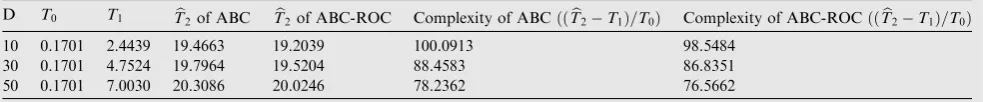
Table 6 Time complexities of the ABC and ABC-ROC algorithms on Rosenbrock function.

D T0 T1 Tb2of ABC Tb2of ABC-ROC Complexity of ABCððTb2T1Þ=T0Þ Complexity of ABC-ROCððTb2T1Þ=T0Þ

10 0.1701 2.4439 19.4663 19.2039 100.0913 98.5484

30 0.1701 4.7524 19.7964 19.5204 88.4583 86.8351

(7)

else slope ==maxROC trace = 0

Step 13:if ﬂag ==maxFlag

Scout bee produces new random solutionxiusing Eq.(3)

resetmaxROCto initialmaxROC

resetmaxTraceto initialmaxTrace

ﬂag = 0

Step 14:Memorize the best solution achieved Step 15:cycle = cycle + 1

Step 16:trace = trace + 1 Step 17:until cycle = MCN

Based on the pseudo-code of ABC-ROC, we set three deci-sion rules to decide the process of scout bee based on the slope’s characters. The decision rules are set as below:

Rule 1:slope¼¼0

Rule 2:slope6maxROCANDslope!¼0 Rule 3:flag¼¼maxFlag

The slope is calculated after trace is equal tomaxTrace. If

the trace is equal to maxTrace, then the slope is calculated

using Eq.(4). If the slope is equal to zero (solution does not

improve), then the ﬁrst rule will be considered where the scout

bee begins searching for a new solution, theflagis incremented

by one and themaxTraceis doubled (the length of the line is

increasing). The increment ofmaxTraceis important to ensure

the slope always there because the slope heavily depends on the maxTrace.

Next, if the slope is less than or equal tomaxROCand the

slope is not zero, then the second rule is applied. In this rule,

the scout bee begins searching for a new solution, and the

max-ROCis set to the current slope. This process is important to

control the presence of the scout bee. If the maxROCis not

set to new value, then the scout bee process always happens and the exploitation will be disrupted.

Finally, if none of the rules applied, the scout bee process

does not occur andmaxROCis set to the current slope. After

that, the ﬂag value needs to be checked. If the ﬂag is equal to maxFlag, then the third rule is applied, where the scout bee

begins searching for a new solution, themaxROCand

max-Traceare reset to the initial value, and the ﬂag is reset to zero. In the event that the solution is not improving, the increment

of ﬂag untilmaxFlagwill help to ﬁnd other new solutions. All

the parameters need to be reset to the initial value because we consider that if this rule is applied, the food sources found by the scout bee is a new solution that should be reassessed. This process will assist the algorithm to escape the local minima at the end of the cycle.

By using slope, we can track the improvement of the result

globally instead of using ‘‘limit”which track the improvement

locally. In addition, we can add a decision rules from the slope’s characters, thus provide more opportunities for scout bee to contribute during the search process.

5. Computational study and discussion

The experiments is conducted to test the parametersmaxROC,

maxTrace and maxFlag with different values. The effect of these parameters is analysed by means of the convergence per-formance and the quality of the solutions obtained from this algorithm.

Further, the ABC-ROC is compared with different state of

art algorithms, including ﬁreﬂy algorithm (FA) (Yang, 2008),

cuckoo search (Cuckoo) (Yang and Deb, 2009) and harmony

search algorithm (HS) (Geem et al., 2001). The FA and

Cuckoo are natural phenomenon algorithm, inspired by the flashing behaviour of fireflies whilst the Cuckoo mimic the

par-asitism behaviour of cuckoo bird laying egg (Yang, 2008; Yang

and Deb, 2009). Comparison with FA and Cuckoo which rep-resent the natural phenomenon algorithm as well as the devel-opment of both algorithm is after the introduction of ABC

Table 7 Effect of the colony size (CS) on the performance of ABC-ROC.

CS Ackley Branin Dixon-Price Griewank Rastrigin

Mean SD Mean SD Mean SD Mean SD Mean SD

4 1.47E+01 4.63E+00 7.02E+00 6.11E+00 2.75E+05 3.44E+05 1.04E+02 7.12E+01 8.84E+01 3.83E+01

6 8.44E+00 4.29E+00 9.53E+00 3.24E+00 5.69E+03 2.03E+04 7.13E+00 1.37E+01 2.44E+01 1.58E+01

12 1.14E01 3.53E01 8.87E+00 2.58E+00 2.32E06 7.63E06 1.57E02 1.81E02 6.30E01 8.46E01

24 3.91E14 3.19E15 2.97E+00 2.24E+00 5.30E15 9.41E15 2.87E03 5.64E03 0.00E+00 0.00E+00

50 3.55E14 4.47E15 7.70E+00 2.51E+00 2.72E15 6.68E16 1.39E03 4.56E03 0.00E+00 0.00E+00

100 3.27E14 3.30E15 5.04E+00 1.65E16 2.78E15 1.20E15 4.07E17 5.44E17 0.00E+00 0.00E+00

200 3.05E14 3.28E15 6.92E+00 1.24E+00 4.27E10 3.66E10 1.48E17 3.84E17 0.00E+00 0.00E+00

CS Rosenbrock Schaﬀer Schwefel Sphere

Mean SD Mean SD Mean SD Mean SD

4 3.11E+07 2.52E+07 2.42E01 2.11E01 -9.52E+03 1.05E+03 1.21E+04 6.11E+03

6 7.02E+05 2.64E+06 3.32E02 6.32E02 1.13E+04 4.89E+02 4.07E+02 8.10E+02

12 2.71E+00 3.40E+00 6.36E04 1.44E03 1.23E+04 1.92E+02 6.95E16 1.20E16

24 5.80E01 1.17E+00 1.48E04 3.69E04 1.26E+04 4.09E+01 5.62E16 1.00E16

50 2.49E01 6.02E01 3.40E06 1.49E05 1.26E+04 1.85E12 5.28E16 8.55E17

100 3.93E02 8.40E02 8.77E08 4.80E07 1.26E+04 1.85E12 4.76E16 8.63E17

200 1.72E02 5.18E02 2.03E06 1.11E05 1.26E+04 1.85E12 4.46E16 7.68E17

(8)

algorithm. For HS algorithm, the comparison is done because HS is developed using different approaches which mimic the

artiﬁcial phenomenon of musical harmony (Geem et al.,

2001). In addition, the comparison is also been done with

ABC and quick ABC (qABC) and the results is taken from Karaboga and Gorkemli (2014).

For a fair comparison, the same parameters setting and

maximum number of evaluation are used, following

(Karaboga and Akay, 2009; Karaboga and Gorkemli, 2014). The colony size is 50 and the maximum number of evaluation

is 500 000. The ‘‘Limit” for ABC and qABC is set to

ðCSDÞ=2 as suggested byKaraboga and Gorkemli (2014).

The Wilcoxon statistical test is carried out on ABC-ROC algorithms to validate the results. The well-known benchmark numerical problems with different characters are considered in order to test the performance of ABC-ROC. The test problems consists of several characters (C), dimensions of the problems (D), the bounds of the search spaces and the global optimum

values. The test problems are presented inTable 1with C

cat-egorized as unimodal-seperable (US), unimodal-nonseperable

(UN), multimodel-seperable (MS) and

multimodel-nonseperable (MN).

Fig. 2 shows the convergence performance of ABC-ROC

with differencemaxROCvalues.

Next, the experiment is conducted to test the performance of individual parameter. The parameters setting is shown in Table 2. This table should be read in the form of a column.

For example, to test themaxROCparameter, both parameters

maxTraceandmaxFlagshould be set to 10 respectively. The results are presented according to the test function.

Table 3shows the mean and standard deviation (SD) for

test problems with different setting of parameter maxROC.

Moreover, the best and worst objective function values are presented in this table.

For all parameter settings ofmaxROC, the ABC-ROC hits

optimum value for Rastrigin problem for each of 30

indepen-dent runs.Table 3presents the results for parametermaxROC.

For Ackley function, ABC-ROC gives the best mean, SD and

worst values formaxROC:0.8and the best values for the

col-umn ‘‘Best”is given bymaxROC:0.6andmaxROC:1.0. For

Branin function the best value for mean, SD and Best are

pro-duced by maxROC:0.2 and maxROC:1.0 whereas the best

value for column ‘‘Worst”are given bymaxROC:0.6and

max-ROC:0.8. For Dixon-Price function the best mean, SD, best

and worst values are produced by maxROC:0.2. The best

results of column ‘‘Best”are given for all parameters with all

settings for Griewank function. For this function, the best

mean, SD and worst are given bymaxROC:0.8. For

Rosen-brock function the best mean, SD and worst are produces by maxROC:0.4whereasmaxROC:1.0given the best for column

‘‘Best”.

For Schaffer function maxROC:0.8 produced the best

Mean, SD, best and worst. For Schwefel function all parame-ter maxROC produced best results in parame-terms of mean, SD, best and worst of 30 independent runs for this function. For Sphere

function, the best mean and best are given by maxROC:0.8

whereas the best SD given bymaxROC:0.4and the best for

column ‘‘Worst”is given bymaxROC:0.2.

The experiment has been done to evaluate the effect of

parameter maxROC of ABC-ROC algorithm. For certain

problems, ABC-ROC produced less different results even with the different setting of parameter. Further, the results for

parameter maxTrace and maxFlag are provided in Tables

A.9 and B.10respectively in Appendix.

In comparison of ABC-ROC with the state of art algo-rithms (Cuckoo, FA, HS, ABC and qABC), the results are

pre-sented inTable 4. The parameters setting for Cuckoo and FA

are based on (Yang, 2014) and for ABC and qABC are

follow-ing (Karaboga and Gorkemli, 2014). For ABC-ROC, the

parameters are set withmaxROC:0.5,maxTrace:100and

max-Flag:50by using trial and error approach. From the table, the mean of 30 independent runs and the standard deviations are presented for considered problems. For a fair comparison, the table values below E-12 are accepted as 0 as in Karaboga and Akay (2009) and Karaboga and Gorkemli (2014).

The best performance of Schaffer function is produced by Cuckoo, where it successfully hits the optimum value. HS duces average performance for all functions and Cuckoo pro-duces average performance for all functions except Schaffer and Sphere. Focusing on ABC-ROC, the best performance for mean is given by Branin function. For Schwefel function, the result produced is the same as ABC and qABC but ABC-ROC produces more consistent results based on the low-est SD value. The result of ABC-ROC on Griewank and Ras-trigin function showed similar results with ABC and qABC.

Results on Table 4 clearly show that ABC, qABC and

ABC-ROC algorithms outperform Cuckoo, FA and HS on the considered test problems. The results also indicate that ABC-ROC outperforms ABC and qABC for certain problems. However, it is not very clear that there is a signiﬁcant differ-ence between the performances of the ABC and ABC-ROC which produced similar results for several problems. Hence, in order to validate the performance of ABC and ABC-ROC, the Wilcoxon signed rank test was used in this paper.

The Wilcoxon test is a nonparametric statistical test to analyse the behaviour of evolutionary algorithms and suitable

for use in small sample size (Garc´a et al., 2009; Kulluk et al.,

2012). The test results are shown inTable 5. The ﬁrst column

represents the test functions. The Second column gives the mean difference between the results of the ABC and qABC and the last column gives the p value that is an important determiner of the test. Since the mean difference column value is 0 for Griewank, Rastrigin and Schwefel functions, there are six test problems that can be discussed. Among them, the p value is different from Rosenbrock is higher that signiﬁcance

Table 8 Comparison between the number of scout bee of

ABC and ABC-ROC.

Function ABC ABC-ROC

Limit =CS*D Limit = (CS*D)/2

Ackley 150 125 24

Branin 834 522 34

Dixon-Price 25 20 24

Griewank 151 76 27

Rastrigin 162 143 11

Rosenbrock 19 8 24

Schaﬀer 321 121 21

Schwefel 143 122 33

Sphere 250 200 24

(9)

level 0.05 which mean this function is not enough evidence to reject the null hypothesis (0.072 > 0.05). These tests show that in these conditions, the performance of ABC-ROC algorithm is significantly better than ABC for another five test functions (Ackley, Branin, Dixon-Price, Schaffer and Sphere). These tests are based on the final results obtained by the algorithms. Generally, we could interpret the simulation and test results as when the three rules are used for scout to search for a new solution, the convergence performance of ABC is significantly

improved in early and late cycles. The effect of parameter

max-Tracecauses the algorithm to escape local optimum in early

cycles and the parameter maxFlag may cause the algorithm

to escape the local optimum during the end of cycles. Hence, a good tuning of the parameters promises much more ﬂexible proﬁle for scout bee and can generate superior convergence performance for ABC-ROC algorithm.

6. Time complexity of ABC algorithms

In this section, a time complexity analysis is carried out for ABC and ABC-ROC on Rosenbrock function. The complexi-ties are calculated for dimensions 10, 30 and 50 as been

sug-gested by Suganthan et al. (2005) and Karaboga and

Gorkemli (2014). The results are shown in Table 6for ABC and ABC-ROC algorithms. This experiment was performed using Windows 7 Professional (SP2) on Intel(R) Core(TM) i7 920 2.67 GHz processor with 6GB RAM and the algorithms were coded by using MATHLAB2014a.

The code execution time for this system was obtained and

demonstrated inTable 6asT0. Next, the computing time for

Rosenbrock function for 200,000 function evaluations is

pre-sented asT1 in the table. Each algorithm was run for 5 times

for 200,000 function evaluations and the average computing

Table A.9 Comparisons of different setting of parameter maxTrace.

maxTrace:20 maxTrace:40 maxTrace:60 maxTrace:80 maxTrace:100

SD 4.14E15 4.03E15 4.25E15 4.34E15 4.13E15

Best 2.93E14 2.93E14 2.93E14 2.58E14 2.58E14

Worst 4.35E14 4.00E14 4.35E14 4.00E14 4.00E14

Branin Mean 8.14E+00 2.69E+00 5.32E+00 3.98E01 5.56E+01

SD 3.77E+00 1.98E+00 2.54E+00 0.00E+00 2.89E14

Best 3.53E+00 4.67E01 2.61E+00 3.98E01 5.56E+01

Worst 1.94E+01 7.78E+00 1.10E+01 3.98E01 5.56E+01

Dixon Mean 2.78E15 2.74E15 2.92E15 2.68E15 2.81E15

SD 4.87E16 5.57E16 8.08E16 4.30E16 5.46E16

Best 2.09E15 1.44E15 1.44E15 1.62E15 1.64E15

Worst 4.27E15 3.60E15 5.20E15 3.60E15 4.09E15

SD 1.35E03 4.17E03 1.35E03 2.25E03 1.88E03

Best 0.00E+00 0.00E+00 0.00E+00 0.00E+00 0.00E+00

Worst 7.40E03 1.97E02 7.40E03 1.23E02 7.40E03

SD 1.82E01 8.35E02 1.42E01 4.93E01 1.34E01

Best 9.84E04 4.51E05 1.29E04 3.12E04 2.75E04

Worst 6.88E01 3.66E01 4.86E01 2.50E+00 5.92E01

SD 1.19E04 2.04E05 2.84E05 1.01E11 6.57E06

Best 0.00E+00 0.00E+00 0.00E+00 0.00E+00 0.00E+00

Worst 6.29E04 8.25E05 1.56E04 5.01E11 3.60E05

SD 1.85E12 1.85E12 1.85E12 1.85E12 1.85E12

Best 1.26E+04 1.26E+04 1.26E+04 1.26E+04 1.26E+04

Worst 1.26E+04 1.26E+04 1.26E+04 1.26E+04 1.26E+04

Sixhump Mean 1.03E+00 1.03E+00 1.03E+00 1.03E+00 1.03E+00

SD 4.16E16 4.16E16 4.40E16 4.29E16 4.29E16

Best 1.03E+00 1.03E+00 1.03E+00 1.03E+00 1.03E+00

Worst 1.03E+00 1.03E+00 1.03E+00 1.03E+00 1.03E+00

SD 8.35E17 8.48E17 9.15E17 1.03E16 8.67E17

Best 2.76E16 3.27E16 3.20E16 2.98E16 3.17E16

Worst 7.13E16 7.36E16 7.22E16 7.02E16 7.16E16

(10)

time of the algorithms are presented asTb2. The algorithm

com-plexities were calculated byðTb2T1Þ=T0.

FromTable 6, the time complexity of ABC-ROC is slightly lower than ABC since the contribution of scout bee causes the number of function evaluations to increase. In addition, the increment rate of ABC-ROC for every dimension is lower than ABC. So, it can be concluded that there is not a strict depen-dence between the dimension of the functions and the com-plexities of ABC-ROC and ABC.

7. Experiment on colony size (CS)

For experiments in this section, the parameters are set same as the previous experiments with the maximum evaluation num-ber = 500,000. The ABC-ROC was tested on the test problems for several colony size: 4, 6, 12, 24, 50, 100 and 200. The results

of this experiment are presented inTable 7.

The best value is written in Bold. Based on Table 7, the

ABC-ROC performs worst when CS is small (CS < 12) except for Schwefel function where the best objective values are pro-duced when CS = 6. For other functions, the good results are obtained by using much larger CS (CS > 12). For Rastrigin function, ABC-ROC hits optimum value when using larger CS (CS > 12). In addition, the results indicate that the ABC-ROC produces best value when CS = 200 for most func-tions (Ackley, Griewank, Rosenbrock and Sphere).

8. Comparison of the number of scout bee

This section discusses the different between parameter ‘‘limit”

of the standard ABC algorithm and maxROC of ABC-ROC

algorithm.Table 8shows the number of scout bees for ABC

and ABC-ROC. ‘‘Limit” for ABC is set to CSD and

ðCSDÞ=2 is suggested by Karaboga and Basturk (2008)

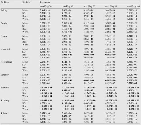
Table B.10 Comparisons of different setting of parameter maxFlag.

maxFlag:20 maxFlag:40 maxFlag:60 maxFlag:80 maxFlag:100

SD 3.58E15 4.27E15 4.38E15 3.81E15 3.90E15

Best 2.93E14 2.93E14 2.93E14 2.93E14 2.93E14

Worst 4.00E14 4.35E14 4.35E14 4.35E14 4.00E14

Branin Mean 5.52E+00 5.56E+01 8.51E+00 3.98E01 3.56E+01

SD 1.87E+00 2.89E14 2.28E+00 0.00E+00 7.23E15

Best 2.73E+00 5.56E+01 6.00E+00 3.98E01 3.56E+01

Worst 1.10E+01 5.56E+01 1.72E+01 3.98E01 3.56E+01

Dixon Mean 2.78E15 2.82E15 2.80E15 2.74E15 2.71E15

SD 6.99E16 6.01E16 5.86E16 6.38E16 5.98E16

Best 9.67E16 2.08E15 1.59E15 1.44E15 1.83E15

Worst 4.07E15 4.30E15 4.09E15 4.54E15 3.87E15

SD 1.35E03 1.35E03 5.52E15 2.72E03 1.23E16

Best 0.00E+00 0.00E+00 0.00E+00 0.00E+00 0.00E+00

Worst 7.40E03 7.40E03 3.03E14 1.49E02 5.55E16

SD 3.46E01 2.39E01 3.23E01 2.55E01 2.51E01

Best 8.14E04 5.41E05 1.72E04 2.77E04 6.71E05

Worst 1.50E+00 1.16E+00 1.53E+00 9.65E01 1.22E+00

SD 1.19E04 8.14E05 1.44E05 1.69E05 1.04E05

Best 0.00E+00 0.00E+00 0.00E+00 0.00E+00 0.00E+00

Worst 6.29E04 4.35E04 5.81E05 8.69E05 5.72E05

SD 1.85E12 1.85E12 1.85E12 1.85E12 1.85E12

Best 1.26E+04 1.26E+04 1.26E+04 1.26E+04 1.26E+04

Worst 1.26E+04 1.26E+04 1.26E+04 1.26E+04 1.26E+04

Sixhump Mean 1.03E+00 1.03E+00 1.03E+00 1.03E+00 1.03E+00

SD 4.23E16 4.10E16 4.40E16 4.29E16 4.34E16

Best 1.03E+00 1.03E+00 1.03E+00 1.03E+00 1.03E+00

Worst 1.03E+00 1.03E+00 1.03E+00 1.03E+00 1.03E+00

SD 8.30E17 7.47E17 1.01E16 1.01E16 9.06E17

Best 2.76E16 4.07E16 3.20E16 3.03E16 3.25E16

Worst 7.13E16 7.29E16 7.38E16 7.44E16 7.44E16

(11)

and Karaboga and Gorkemli (2014), respectively. For ABC-ROC, maxROC is set to 0.8, maxTrace is to 60 and maxFlag is to 100.

Based onTable 8, the number of scout bees of ABC-ROC is

less than ABC. However, the results from Table 11 indicate that ABC-ROC is capable to produce results better than or similar to those of ABC algorithm. This indicates that the ABC-ROC has reduced the usage of scout bee but able to pro-duced better results.

9. Conclusion

This paper presents a new definition of the scout bee process, replacing the parameter limit of the standard ABC. The algo-rithm is called ABC-ROC, that keeps track the changing of the slope on the performance graph. Experimental studies indicate that the new definition significantly improves the convergence

performance of the ABC when the parametersmaxROC,

max-Trace and maxFlag are set appropriately. These additional parameters give more ﬂexible approach and make the scout bee to be more presence during the search process.

The performance of the ABC-ROC is compared with that of the standard ABC and other state of the art algorithms. The results indicate that the ABC-ROC produces promising results for considered problems. Moreover, the effect of colony size and the complexity is carried out. The ABC-ROC can be considered as an alternative approach for optimization prob-lems. In the future, the performance of ABC-ROC can be tested with more complex problem such as classiﬁcation, clus-tering and neural network.

Acknowledgements

The authors wish to thank Universiti Teknologi Malaysia (UTM) under Research University Grant Vot-02G31 and Ministry of Higher Education, Malaysia (MOHE) under the Fundamental Research Grant Scheme (FRGS Vot-4F551) for the completion of the research.

Appendix A. Comparisons of different setting of parameter maxTrace

SeeTable A.9.

Appendix B. Comparisons of different setting of parameter maxFlag

SeeTable B.10.

References

Aderhold, A., Diwold, K., Scheidler, A., Middendorf, M., 2010. Artiﬁcial bee colony optimization: a new selection scheme and its performance. In: Nature Inspired Cooperative Strategies for Optimization (NICSO 2010). Springer, pp. 283–294.

Akay, B., Karaboga, D., 2012. A modified artificial bee colony algorithm for real-parameter optimization. Inf. Sci. 192, 120–142. Basturk, B., Karaboga, D., 2006. An artificial bee colony (abc)

algorithm for numeric function optimization. In: IEEE Swarm Intelligence Symposium, pp. 12–14.

Bullinaria, J.A., AlYahya, K., 2014a. Artiﬁcial bee colony training of neural networks: comparison with back-propagation. Memet. Comput. 6 (3), 171–182.

Bullinaria, J.A., AlYahya, K., 2014b. Artiﬁcial bee colony training of neural networks. In: Nature Inspired Cooperative Strategies for Optimization (NICSO 2013). Springer, pp. 191–201.

Garc´a, S., Molina, D., Lozano, M., Herrera, F., 2009. A study on the use of non-parametric tests for analyzing the evolutionary algo-rithms behaviour: a case study on the cec2005 special session on real parameter optimization. J. Heurist. 15 (6), 617–644.

Geem, Z.W., Kim, J.H., Loganathan, G., 2001. A new heuristic optimization algorithm: harmony search. Simulation 76 (2), 60–68. Hanbay, K., Talu, M.F., 2014. Segmentation of sar images using improved artiﬁcial bee colony algorithm and neutrosophic set. Appl. Soft Comput. 21, 433–443.

Karaboga, D., Akay, B., 2009. A comparative study of artiﬁcial bee colony algorithm. Appl. Math. Computat. 214 (1), 108–132. Karaboga, D., Basturk, B., 2007. A powerful and efﬁcient algorithm

for numerical function optimization: artiﬁcial bee colony (abc) algorithm. J. Global Optimizat. 39 (3), 459–471.

Karaboga, D., Basturk, B., 2008. On the performance of artiﬁcial bee colony (abc) algorithm. Appl. Soft Comput. 8 (1), 687–697. Karaboga, D., Gorkemli, B., 2014. A quick artiﬁcial bee colony (qabc)

algorithm and its performance on optimization problems. Appl. Soft Comput. 23, 227–238.

Karaboga, D., 2005. An idea based on honey bee swarm for numerical optimization, Techn. Rep. TR06, Erciyes Univ. Press, Erciyes. Kashan, M.H., Nahavandi, N., Kashan, A.H., 2012. Disabc: a new

artiﬁcial bee colony algorithm for binary optimization. Appl. Soft Comput. 12 (1), 342–352.

Kong, X., Liu, S., Wang, Z., 2013. An improved artiﬁcial bee colony algorithm and its application. Int. J. Signal Process. Image Process. Pattern Recognit. 6 (6).

Kran, M.S., Fndk, O., 2015. A directed artiﬁcial bee colony algorithm. Appl. Soft Comput. 26, 454–462.

Kulluk, S., Ozbakir, L., Baykasoglu, A., 2012. Training neural networks with harmony search algorithms for classiﬁcation prob-lems. Eng. Appl. Artiﬁc. Intell. 25 (1), 11–19.

Lee, W.-P., Cai, W.-T., 2011. A novel artiﬁcial bee colony algorithm with diversity strategy. In: Natural Computation (ICNC), 2011 Seventh International Conference on, vol. 3. IEEE, pp. 1441–1444. Lei, X., Huang, X., Zhang, A., 2010. Improved artiﬁcial bee colony algorithm and its application in data clustering. In: Bio-Inspired Computing: Theories and Applications (BIC-TA), 2010 IEEE Fifth International Conference on. IEEE, pp. 514–521.

Luo, J., Wang, Q., Xiao, X., 2013. A modified artificial bee colony algorithm based on converge-onlookers approach for global optimization. Appl. Math. Computat. 219 (20), 10253–10262. Maeda, M., Tsuda, S., 2015. Reduction of artificial bee colony

algorithm for global optimization. Neurocomputing 148, 70–74. Ozturk, C., Karaboga, D., 2011. Hybrid artiﬁcial bee colony algorithm

for neural network training. In: Evolutionary Computation (CEC), 2011 IEEE Congress on. IEEE, pp. 84–88.

Ozturk, C., Hancer, E., Karaboga, D., 2015. Dynamic clustering with improved binary artiﬁcial bee colony algorithm. Appl. Soft Comput. 28, 69–80.

Stanarevic, N., 2011. Comparison of different mutation strategies applied to artiﬁcial bee colony algorithm. In: Proceedings of the European computing conference (ECC11), pp. 257–262.

Stanarevic, N., Tuba, M., Bacanin, N., 2010. Enhanced artiﬁcial bee colony algorithm performance. In: Proceedings of the 14th WSEAS International Conference on Computers: Part of the 14th WSEAS CSCC Multiconference, vol. 2, pp. 440–445.

(12)

Xiang, W.-L., An, M.-Q., 2013. An efﬁcient and robust artiﬁcial bee colony algorithm for numerical optimization. Comput. Operat. Res. 40 (5), 1256–1265.

Yan, X., Zhu, Y., Zou, W., Wang, L., 2012. A new approach for data clustering using hybrid artiﬁcial bee colony algorithm. Neurocom-puting 97, 241–250.

Yang, X.-S., 2008. Fireﬂy algorithm. Nature Inspired Metaheuristic Algorithms 20, 79–90.

Yang, X.-S., 2014. Cuckoo search and firefly algorithm: Overview and analysis. In: Cuckoo Search and Firefly Algorithm. Springer, pp. 1–26.

Yang, X.-S., Deb, S., 2009. Cuckoo search via le´vy ﬂights. In: Nature & Biologically Inspired Computing, 2009. NaBIC 2009. World Congress on. IEEE, pp. 210–214.

Zhao, H., Pei, Z., Jiang, J., Guan, R., Wang, C., Shi, X., 2010. A hybrid swarm intelligent method based on genetic algorithm and artiﬁcial bee colony. In: Advances in Swarm Intelligence. Springer, pp. 558–565.