Optimized-Hilbert for mobility in wireless sensor networks

OPTIMIZED-HILBERT FOR MOBILITY IN WIRELESS

SENSOR NETWORKS

Maznah Kamat

1

Abdul Samad Ismail

2

Stephan Olariu

3

1,2_{Faculty of Computer Science and Information Systems,}

Universiti Teknologi Malaysia, 81310, UTM Skudai, Johor Darul Ta’zim 3_{Department of Computer Science,}

Old Dominion University, Norfolk, VA 23529-0162 U.S.A.

E-mail: {

1

maznah,

2

abdsamad}@utm.my;

3

[email protected]

Abstract

In wireless sensor networks (WSNs), mobilizing sink node for data collection can minimize communication and maximize network lifetime. Several mobility algorithms have been proposed to control sink node’s movement. However, they do not consider mobility for coverage area problem. Hilbert space-filling curves technique is modified to navigate mobile sink in traversing specfiic area of the sensor field. The algorithm is called optimized-Hilbert, which provides mobility pattern of a sink node in covering an ellipsoidal monitoring area during data collection for a specific mission by traversing the entire area from an entry point and finish at an exit point of square grids. The optimized-Hilbert requires less number of steps as compared to conventional Hilbert. Additionally, it is also compared with circular mobility, and result indicates the efficiency of optimized Hilbert.

Keywords: Wireless sensor networks, area covering, mobile base station, mobility pattern.

1. Introduction

As envisaged by Mark Weiser that the most useful computer would be an invisible one [19]. Various research and engineering effort especially in hardware has been put forth to bring the vision a reality. Today, a collective of tiny motes called sensor nodes with the capability of sensing environment, processing, and communicate form a new networking technology called Wireless Sensor Networks (WSNs). This networking is revolutionizing the traditional method of data collection, and is gaining popularity for their potentially low-cost solution to a variety of real-world challenges [1,2,3]..

Location based application such as spatial query of gas stations in a district requires information about the locations of the gas stations from a wide region. However, spatial query of gas stations within 1 mile radius from the center of a district requires finer

extraction of detailed location of smaller region. Thus, the application must be able to zoom in from coarser region to finer region. Data from finer region must be collected and aggregated for the purpose of such application.

Current literatures on exploiting mobile sink for data collection focus on mobility for maximizing WSNs lifetime. This paper focuses on utilizing mobile sink not only for maximizing WSNs lifetime but include coverage problem. A powerful device called aggregation and forwarding node (AFN) is defined as in [5] which acts as a mobile sink that cover the monitoring area. It collects sensor reading, which are relayed to a particular location along the grid that it traverses. AFN utilizes Hilbert space-filling curve in controlling its movement within the area of interest represented as an ellipse. The AFN will only collect data once from a region within its R

transmission range. in a particular order in satisfying a query of a specific mission such as providing locations of a dangerous event e.g. fire. Based on the gathered information, in-situ users can plan its’ safe path.

The organization of the paper is as follows: Section 2 discusses the existing solutions of mobile sink in maximizing WSNs lifetime. Section 3 provides a proposed design of AFN mobility in covering the entire monitoring area and Section 4 presents concluding remarks.

2.

Background

This section provides brief preliminaries of related works on sensing coverage and mobility.

2.1. Sensing coverage

Sensing coverage is a measured Quality of Service of sensor field which reflects how well an area is monitored or tracked. Due to limited sensing range of the sensor nodes, sensors must be appropriately deployed to achieve adequate coverage level to properly perform sensing task. In random deployments, deployed sensors are scattered due to uncontrolled landing position when dropped from

Fifth International Conference on Computational Science and Applications

an airplane which may cause coverage holes. The work of Huang et al [6] consider coverage problems as sensing region, whereby distributed deployment of sensors should sufficiently cover target area given k-sensors.

To maximize covered area, sensor is mobilized to cover a coverage hole [7]. In [7] coverage hole is discovered by employing Voronoi diagrams. Protocols were designed to move the sensor to the target area from densely deployed to sparsely deployed area. Liu et al [27] studied the effect of mobile sensor to network coverage which include detecting randomly located target.

2.2. Mobility for data collection

In a remote monitoring environment, data collected from the sensing region must be relayed to the static BS which resides either inside the field or on the periphery of the field. The following sub-section discussed mobility strategies employed by various categories of exploiting mobile BS for data collection which leads to sustainable network lifetime. According to [4], the various mechanisms are broadly classified as mobile base station (MBS), mobile data collector (MDC), and rendezvous.

2.2.1. Mobile base stations. Stationary multiple-BSs are moved to another feasible site at each round as proposed by Shashidhar Rao et al [8]. However, computation of new location is based on inductive logic programming (integer linear programming), which the author found to be time consuming. In the work of Jun Luo et al [9], several movement strategies of a single base station were explored − arbitrary movement, optimum mobile strategies along periphery for circular sensor deployment, and circular trajectory inside deployment area. Circular deployment is not considered a general representation of monitoring area, while the movement concept of appears everywhere with the same frequency is not required for one-time data collection.

2.2.2. Mobile data collector. For large area with sparse sensors deployment, mobile sink reduce relaying to one-hop whereby the mobile sink will visit individual sensor node to collect data reading. Mobility pattern of a sink node under this category can be sub-classified as randomized, predictable, and controlled [17,18,19].

For a randomized mobile data collector, the work of [20] proposed three-tier architecture. The mobile sink nodes are model as the middle-tier which collects data reading from sensor nodes at bottom-tier. Two-dimensional grid is used to place the nodes in creating network topology. Mobile sinks can move to any four directions from its current grid position, with equal probability. Due to randomization mobility based on

equal probability, it is unclear whether it can guarantee an in-order traversal.

Mobility of sink node is not computed on demand, sink node follow a predetermine path such as bus route to collect data from sensor field [21,22]. Sensor nodes that are not within range will not be able to communicate with mobile sink to deliver data reading. Thus, this type of predictable mobility is not suitable for a critical application.

Several works on controlled mobility were designed [17,18]. In the work of [17], mobile sink slows down whenever sensor nodes density is low, increase its speed otherwise. Mobile sink follows a simple path to reduce number of hops in relaying data. The paper did not discuss in detail the movement pattern. Mobility of sink is based on deadline [18], whereby mobile sink visits sensor node before sensor’s buffer becomes full. The sensor nodes may be revisited based on frequency of data sampling, which influence the deadline. To control sink movement, node with closest deadline will be visited first. The algorithm may cause a missed deadline, which leads to miscollection of could be a critical data.

Optimized mobile data collector [13] tries to minimize data loss (similar to the work of [11]) but consider a situation when mobile sink moves slowly. To avoid buffer overflow, an algorithm called Partitioning Based Scheduling will initially groups nodes that have similar buffer overflow times into bins Bi _{and then the grouped}

nodes are partition into 2i-1 _{sub-bins using 2-d tree in such}

a way they are closely located. Computation of visiting schedule is performed in two steps − path for sub-bin is calculated using TSP for single traversal, and each sub-bin path of B j

i is concatenated with every bin of Bi which

relate to frequency of visits called cycles. Calculation of the minimum speed of mobile sink depends on number of cycles. Simulation result shows the performance of the algorithm in [15]. Multiple visits to the same nodes cause unnecessary redundant data collection, which does not satisfy one-time data collection.

2.2.3. Rendezvous. Rendezvous is a hybrid solution which combine both methods − mobile base station and mobile data collector [4]. Data are accumulated at designated sensor nodes, which buffer the data as in MDC and relayed multi-hops as in MBS. This approach causes data latency because generated data are buffered before they are relayed multi-hops to mobile sink. In addition, buffer must be large enough to store the data. To the best of our knowledge, none literature are available for this type of category.

3.

AFN mobility

data reading, and aggregate collected data from nearest neighbors. These requirements cannot be fully satisfied by the approaches discussed above. To fulfill the requirement, the system must address the following

issues: i. How would the area of interest be represented

mathematically?

ii. How would the monitoring area be covered?

iii How does AFN computes its’ trajectories in ensuring the entire area is covered?

In this work, the following assumptions are made: i. Single AFN is responsible for covering the area of

interest

ii. Movements of AFN is controlled and restricted/confined to simple directions − left, right, up and down along the square grid.

iii. Sensing coverage is accurate

iv. An existing routing algorithm [16] is employed.

This optimized Hilbert-based mobility is classified as rendezvous mobility.

3.1 Monitoring area of interest

In-situ user selects the area of interest by inscribing the map on the monitor screen. The system computes the path to cover the entire area and send it as a request to an AFN, which will satisfy the user request called a mission. The area of interest is the region signified/represented as an ellipse. The ellipse is mapped into square grid with an associated coordinates. Equation (1) is a general form of an ellipse with a center at (h,k) [17]:

(

x−h

) (

2+ y−k

)

2 =1

(1) 2

a

b2

In this work, a titled ellipse is considered. A generalized equation for a tilted ellipse as expressed by equation (2), applies [17]:

( )

( )

(

)

(

xcos_θ +ysin_θ −h'

)

2+ 2

a

( )

(

)

( )

(

ycosθ −xsinθ −k'

)

2 =1

(2) 2

b

where

h

'

and

k

'

are defined as follow:

(

+

)

(

θ +α

)

= cos

' h2 k2

h

_k'=

(

_h2+_k2

)

sin

(

θ +α

)

An ellipse represents a more generalize shape as compared to a circle, which poses symmetric quadrants (value of a is equal to b as in equation (1)). An ellipse is

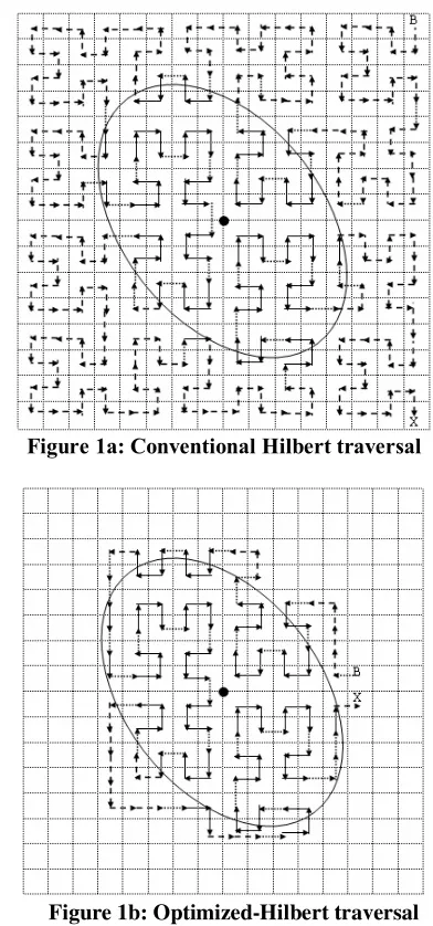
commonly used in determining a monitoring area of interest. U.S. Environmental Protection Agency in Detroit, Michigan is conducting a study, named the Detroit Exposure and Aerosol Research Study (DEARS) [18]. In the study, some of the monitoring areas are indicated by ellipses labeled from 1 to 6 on map of Detroit. Hence, referring to figure 1, this study adopted an ellipse to represent an area of interest, while a circle represents the omni-directional antenna attached to the AFN with limited radius of transmission R

Figure 1a: Conventional Hilbert traversal

Figure 1b: Optimized-Hilbert traversal

3.2 Traversing the monitoring area

R gridSize= 2*

The AFN will traverse the ellipsoidal area and make a stop at each square grid for a period of time t. During time

t, sensors within the circle of R radius (within AFN transmission range) will route data to the overlapped section covered by AFN. The data are gathered and after time t, the AFN changes its direction as specified by the Hilbert-based algorithms explained in sections 3.3 and 3.4. Figures 1a and 1b illustrate the path AFN takes for conventional Hilbert and optimized-Hilbert respectively in covering the ellipsoidal area. In the figures different type of arrows − the dash arrows connect separated Hilbert cells, dotted arrows indicate entering a Hilbert cell, while solid arrows describe connectivity of conventional Hilbert cells. In conventional Hilbert each cell is visited once, but optimized-Hilbert allows multiple visits to cell but AFN will only collect data once.

3.3 Conventional space-filling curves

Hilbert space-filling curves is applied in various areas of research such as traveling salesman problems [24], pattern and texture analysis [25], and data compression [26].

HA HB

HD HC

Figure 2: Curve node label − A, B, C, and D

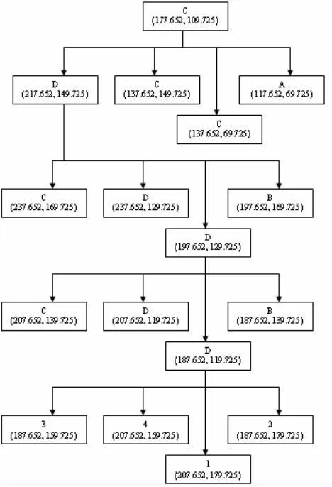
The basic 2 x 2 Hilbert curves is shown in figure 2 which describe the mobility pattern stores in each node of the Hilbert tree built as shown in figure 3. Figure 3 is an example of the tree when an ellipse (axes 40-60) centered at coordinate (177.652, 109.725) is used. The tree is built based on sub-trees pattern. Parent node can be A, B, C, or D. Node A has children of node B, A, A, and C for respective quadrants 1, 2, 3, and 4. Children of node B are A, B, B, and D for quadrant 1, 4, 3, and 2. If node C is a parent of a sub-tree, it generate children of node D, C, C, and A for its quadrants 3, 2, 1, and 4. Sub-tree of node

D consists of children nodes − C, D, D, and B for its quadrant 3, 4, 1, and 2.

Figure 3: Partial Hilbert tree for the AFN traversal

Based on the sub-tree, the following procedure recursively builds the conventional Hilbert tree:

i. Compute range of square required in covering the ellipse (xB and xX)

ii. Based on xB and xX, determine Hilbert curve width (W)

iii. Build complete Hilbert tree based on the value of W (partial tree is shown in figure 3):

a. Compute tree height (H) based on value of W

b. Build first level Hilbert tree

c. Add second level Hilbert tree to first. d. Recursively build next tree level while level

is less than height:

e. When level is equal to height, assign leaf node with the center coordinate of cell (xc,yc) and order of quadrant (which represent the direction of movement).

3.4 Optimized-Hilbert space-filling curves

Inspired by the travelling salesman problems, Hilbert space-filling curve is used in covering the ellipse, which is mapped to square grid called Hilbert cell. Each square grid will be covered by a circle. Mathematically, the circle, which represents the AFN will have to cover the ellipse. To provide in-order traversal, the AFN will track the route pre-computed as follow (assuming conventional Hilbert tree is built):

i. Identify square grid that lies within an ellipse: for xn Å xB; xn < xX; xnÅ xn +gridSize

a. Determine low and high y coordinate of bounded ellipse (yn), where n = low .. high

as describe in algorithm B

b. Search Hilbert tree of all leaf nodes for a match such that (xn, yn) = (xc,yc)

c. For a match in b, set a flag

ii. Prune Hilbert tree so that only leaf nodes that are within an ellipse represent the path to be taken by AFN:

a. Traverse the Hilbert tree recursively until leaf nodes are reached

b. If flag of leaf node is not set, delete the node from the tree

Algorithm B – the low and high grid bounded by ellipse can easily be obtained by employing simultaneous equations technique. The roots of two equations are the intersection of straight line and ellipse which are computed as follow:

i. compute a,b and c ii. ABC Å

(

b2 −4ac

)

iii. if ABC > 0

low Å −b−ABC a 2 high Å −b+ABC

a 2

Travel distance of AFN relies on the steps count:

gridSize count

steps dist

AFN_ = _ * (3)

3.5 Circular traversal

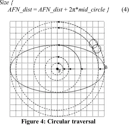
The mobility pattern utilizes in the work of [22,23] is circular-based, which is of controlled mobility strategy. Figure 4 depicts the adopted controlled mobility pattern applied to ellipsoidal coverage for an area with axes 80-40. The smaller circle (i.e AFN) will move along the dotted larger circle in anti-clock wise direction. The radius of outermost circle and the innermost circle are set to 8*gridSize, 1*gridSize respectively. AFN will traverse

along the circle starting from outermost circle to innermost circle, begin from point B and finish at point F. Circular mobility causes some area to be visited even if they are outside ellipse boundary. Procedure below simply calculates the traveled distance of AFN:

for mid_circle = outer_radius*gridSize to inner_radius *gridSize {

AFN_dist = AFN_dist + 2π*mid_circle } (4)

Figure 4: Circular traversal

4. Simulation results

Based on the algorithm described in section 3.3 and 3.4, the following specifications are used during the simulation in determining the steps count of AFN traversal:

i. Equations for the titled ellipse

Various sizes of ellipses are created by changing the value of semi-minor and semi-major axes, and angle of rotations (0-180).

ii. Straight line equations range from xB to xX. iii. A circle with a radius R that cover the square

grid.

iv. Deployment area of 160 x 160.

same count too e.g steps count for ellipses with axes 60-80, and axes 80-60 rotated by 450 _{is 191. However, with} conventional Hilbert algorithm, the step counts remain the same (i.e 256) irrespective of the size of an ellipse.

0 50 100 150 200 250 300

0 15 30 45 60 75 90 105 120 135 150 165 180

Conventional Hilbert40-60 Hilbert60-40 Hilbert50-70 Hilbert70-50 Hilbert60-80 Hilbert80-60

Figure 5: Number of steps of traversal

Based on equations (3) and (4), traveled distances of AFN are tabulated. Table 1 shows that AFN distances traveled are constant for both mobility strategies − conventional Hilbert, and circular, irrespective of the ellipse shapes. For optimized-Hilbert, AFN’s traveled distance decreases as the ellipse shape becomes narrower. This is in contrast to circular movement, which causes the AFN to travel at longer distance. Thus, optimized-Hilbert is adaptive to axis.

Table 1. AFN’s traveled distance Distance (gridSize=10) Shape /

Mobility

strategy Circular Conventional Hilbert

Optimized Hilbert Hilbert

(80 – 60) 1808.36 2560 1840

Hilbert

(80 – 40) 1808.36 2560 1270

Hilbert (80 – 25)

1808.36 2560 1000

5. Conclusion and future works

This paper addressed the problem of mobilizing BS in a target field in ensure gathering of one-time data collection. Based on conventional Hilbert space-filling curves, optimized-Hilbert is achieved by pruning the conventional Hilbert-tree which enables AFN to move from an entry point to exit point and covering only specific area of interest i.e the elliptical area. Simulation results verified the efficiency of optimized-Hilbert mobility compared to circular mobility.

The direction of next research is to train sensors as the AFN stops at each cell for data gathering and aggregation.

References

[1] Jessica D. Lundquist1, Daniel R. Cayan1,2, and Michael D. Dettinger, “Meteorology and Hydrology in Yosemite National Park: A Sensor Network Application”, IPSN 2003, LNCS 2634, pp. 518–528, 2003, Springer-Verlag Berlin Heidelberg 2003

[2] K. Martinez, P. Padhy, A. Riddoch, H.L.R. Ong and J.K. Hart, “Glacial Environment Monitoring using Sensor Networks”, REAL WSN’05, June 21–22, 2005, Stockholm, Sweden., ACM 2005.

[3] A. Mainwaring, J. Polastre, R. Szewczyk, D Culler, and J. Anderson, ” Wireless Sensor Networks for Habitat Monitoring,”

WSNA’02, September 28, 2002, Atlanta, Georgia, USA. ACM 2002.

[4] Eylem Ekici, Yaoyao Gu, and Doruk Bozdag, “Mobility-Based Communication in Wireless sensor Networks”, pp 56-62. IEEE Communications Magazine, July 2006.

[5] S. Olariu, M. Eltoweissy, and M Younis, “ ANSWER: Autonomous Wireless Sensor Network”, Proc of Q2SWinet’05, October 13, 2005, Montereal, Quebec Canada, ACM 1-59593-341-0/05/0010.

[6] Chu-Fu Huang, and Yu-Chee Tseng, “The Coverge problem in a Wireless Sensor Network”, Mobile networks and Applications 10-519-528, Springer 2005.

[7] Guiling Wang, Guohong Cao, and Tom La Porta, “Movement-Assisted Sensor Deployment”, IEEE INFOCOM 2004.

[8] Shashidar Rao Gandham, Milind Dawande, Ravi Prakash and S. Venkatesan, “ Energy efficient Schemes for Wireless Sensor Networks with Multiple Mobile base Stations”, GLOBECOM 2003, pp 377381, IEEE 2003.

[9] Jun Luoand Jean-Pierre Hubaux, “Joint Mobility and Routing for Lifetime Elongation in Wireless Sensors Networks“, IEEE 2005, pp 1735-1746.

[10] Aman Kansal, Arun A Somasundra, david D jea, Mani B Srivastava and Debroh Estrin, “Intelligent Fluid Infrastructure for Embedded Networks”, ACM MobiSYS ’04, June 6-9, 2004 Boston, Massachusetts, USA. ACM 2004 1-1-58113-793.

[11] Arun A. somasundara, Aditya Ramamoorthy, and Mani B. Srivastava, “Mobile Element Scheduling fro Efficient Data Collection in Wireless Sensor Networks with Dynamic Deadlines”, Proc 25th _{IEEE Real_Time Sys. Sysm., 2004.}

[13] Rahul C Shah, Sushanat Jain, and Waylon Brunette, “ Data MULEs: Modeling a Three-tier Architecture for Sparse Sensor Networks”, IRS-TR-03-001, January, 2003.

[14] Eylem ekici, Yaoyao Gu, and Doruk Bozdag, “Mobility-based Communication in Wireless Sensor Networks”, IEEE Communications Magazine, July 2006.

[15] Arnab Chakrabarti, Ashutosh Sabharwal, and Behnaam Aazhang,”Using Predictable Observer Mobility for Power Efficient Design of Sensor Networks”, Information Processing in Sensor Networks, Second International Workshop, IPSN 2003, Palo Alto, CA, USA, April 22-23, 2003, Springer pp 129-145 2003, ISBN 3-540-02111-6.

[16] A Wadaa, S Olariu, L Wilson, M. Eltoweissy, and K Jones, “Training a Wireless Sensor Network”, Mobile Networks and Applications 10, 151–168, 2005, Springer Science.

[17] Lyman M. Kells and Herman C. Slotz, “Analytic Geometry”, Prentice Hall 1949.

[18] Detroit Exposure and Aerosol Research Study (DEARS), http://ww.epa.gov/dears. Last updated on Friday, March 10th, 2006

[19] M. Weiser, “ The computer for the 21st _Century”,

Scientific American, pages 94-104, September 1991.

[20] Maznah Kamat, Abd Samad Ismail, and Stephan Olariu, “Hilbert Space-Filling Curves on Covering an Ellipse”, Post Graduate Seminar PARS07, Faculty of Computer Science and Information Systems, Universiti Teknologi Malaysia, 2nd_-5th

July 2007.

[21] Guiling Wang, Guohong Cao, and Tom La Porta, “Proxy-based Sensor Deployment for Mobile Sensor Networks”, IEEE 2004.

[22] Jernej Polajnar(#), Tyler Neilson, Xiang Cui, and Alex A. Aravind, “Simple and Efficient Protocols for Guaranteed for Message Delivery in Wireless Ad-Hoc Networks”, IEEE 2005.

[23] Arun Somasundara, Aman Kansal, David Jea, Mani Srivastava, “Controlled Mobility for Increased Controlled Mobility for Increased Lifetime in Wireless Sensor Networks Lifetime in Wireless Sensor Networks”, http://nesl.ee.ucla.edu.

[24] Gao, J. and Stelee, J. M. 1994, ”General space-filling curve heuristics and limit theory for the traveling salesman problem.”, J. Complexity 10, 2 (June), 230-245.

[25] Abend, K., Harley, T. J., and Kanal, L. N. 1965. Classification of binary random patterns. IEEE Trans. Inf. Theor. IT-11, 4 (Oct.), 538–544.

[26] Moghaddam, B., Hintz, K. J., and Stewart, C. V. 1991. Space-filling curves for image compression. In Proceedings of the SPIE. 414–421.