A Comparative Analysis of Partial Least Squares (PLS) Regression and Artificial Neural Network (ANN) Methods for Determining Elemental Weights in Sheet Metal.

(1)

ABSTRACT

BOND, BENJAMIN DANIEL. A Comparative Study of Partial Least Squares (PLS) Regression and Artificial Neural Network (ANN) Methods for Determining Elemental Weights in Sheet Metal. (Under the direction of Dr. Robin P. Gardner).

(2)

(3)

A Comparative Study of Partial Least Squares (PLS) Regression and Artificial Neural Network (ANN) Methods for Determining Elemental Weights in Sheet Metal

by

Benjamin Daniel Bond

A thesis submitted to the Graduate Faculty of North Carolina State University

in partial fulfillment of the requirements for the degree of

Master of Science

Nuclear Engineering

Raleigh, North Carolina

2014

APPROVED BY:

_______________________________ ______________________________

Dr. Robin P. Gardner Dr. John Mattingly

Committee Chair

(4)

Dedication

(5)

Biography

(6)

Acknowledgements

I would like to extend my thanks to Dr. Robin Gardner for allowing me the opportunity and latitude to work on this topic. It is rare that one can pursue something out of pure intellectual curiosity, but you were able to allow me this experience, so thank you very much. I would also like to thank Dr. John Mattingly; your knowledge and expertise was immensely helpful and I’ve learned so much from you over this past year. My only regret is not taking more of your classes. Dr. Smith, thank you for taking me on as an advisee on such late notice. I really appreciate your openness and desire to help me achieve this goal.

I would also like to thank the numerous students that played a special role in my work. This honor goes to Mital Zalavadia, Dr. Kyoung Lee, Adan Calderon, and Guojing Hou for their in-depth instruction, late night discussions, hands on help, and moral support.

There are a few professors who made a profound impact on me, and without their help none of this would have been possible. They deserve mentioning and include Dr. Mohammad Bourham, Dr. Hany Abdel-Khalik, Dr. Dmitry Anistratov, Dr. Joseph Doster, Dr. Moody Chu, Dr. Jerome Lavell, Dr. Yara Yingling, and Mr. Scott Lassel. Thank you for everything.

Special thanks to the Rick Lamy and Terry Briggs at the precision instrument machine shop for making the custom laser mounts needed for this experiment.

A big thank you to those at the NC State Craft Center who gave me guidance in my construction of the target, source, and detector holding device; not only was it functional, but it came out quite beautifully for a novice craftsman.

(7)

by means of my first internship opportunity, access and help in obtaining scholarships, and exclusive access to research opportunities. Beyond that, she has been a staunch supporter of my education and she and Sherry Bailey were to first to make me realize that graduate school was a very real possibility for me.

(8)

List of Tables

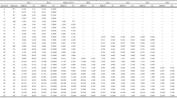
Table 1 – Select X-ray transition energies (in KeV) ... 8

Table 2 – Metals used in the simulation ...30

Table 3 – Settings for the Experimental Equipment ...32

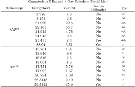
Table 4 – Characteristic Xray and gamma ray emissions for Cd109_{and Am}241_...35

Table 5 – Gaussian broadening parameters ...36

Table 6 – Metals used in the experiment ...37

Table 7 – Performance Table for the Stainless Steel Set of X-ray spectroscopic data ...44

Table 8 – PLS Model – LV Study (w/o Scaling or Centering) ...46

Table 9 – Mean of Square Error between Model Estimates and Data ...48

Table 10 – Selected Results for aluminum 1100 and 7075 ...49

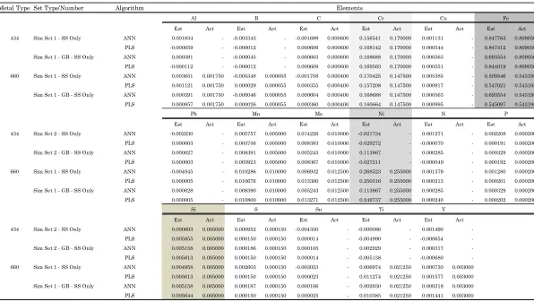
Table 11 – Selected Results for stainless steel 316 ...50

Table 12 – Selected Results for stainless steel 434 and 660, using all of the metals as a basis for training ...51

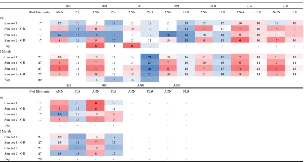
Table 13 – Number of elements predicted in the steel samples that were within the range of the ASTM Standard* ...53

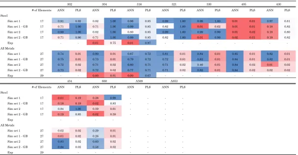
Table 14 – Fraction of elements predicted in the steel within the range of the ASTM Standard* multiplied by their contribution ...54

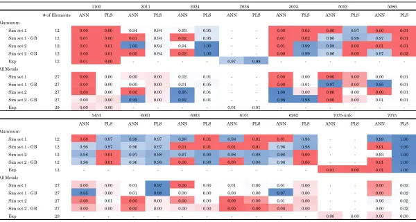
Table 15 – Fraction of elements predicted in the aluminum within the range of the ASTM Standard* multiplied by their contribution ...55

Table 16 – Fraction of elements predicted in the copper based metals within the range of the ASTM Standard* multiplied by their contribution ...56

Table 17 – ASTM Standards for Select Types of Copper Based Metals ...70

Table 18 – ASTM Standards for Select Types of Copper Based Metals ...71

Table 19 – ASTM Standards for Select Types of Aluminum ...72

Table 20 – PLS Model - LV Study - Centered and Scaled Data Input ...73

Table 21 – Estimate of Set 1 Aluminum Element Weight Fractions (8 Node ANN Model with Set 2 Simulated Data) ...74

(11)

(12)

(13)

(14)

List of Figures

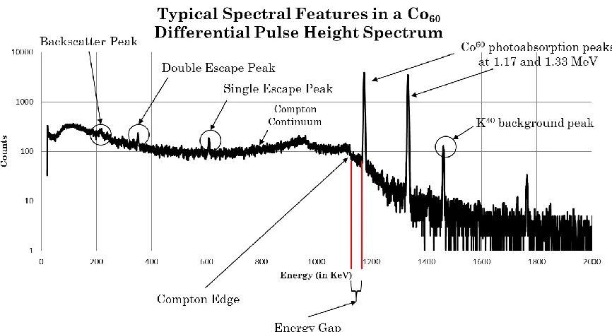
Figure 1 – Typical Features seen in a Gamma Spectra of Co-60 ... 3

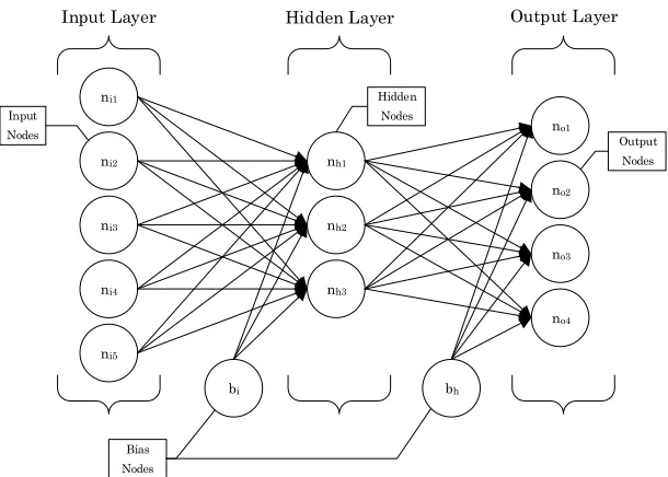
Figure 2 – Typical Structure of a Feed-Forward Neural Network ...10

Figure 3 – Structure of Neural Net used in this study and its transformation functions. ...11

Figure 4 – X and Y data block structure ...12

Figure 5 – Sigmoid function Figure 6 – Error Function ...13

Figure 7 – Flow Diagram of the ANN Algorithm ...20

Figure 8 – MCNP Model of a LEGe Detector, Metal Target, Cd-109 X-ray Source, and Lead Collimator ...27

Figure 9 – Russian Roulette Psuedo Code ...29

Figure 10 – Block Diagram of the Experimental Setup...31

Figure 11 – Perspective view of lead collimator...32

Figure 12 – Side view of detector, target, and collimator ...33

Figure 13 – View of Experimental setup with lasers mounted ...34

Figure 14 – Experimental setup with laser dots aligned on the metal surface ...34

Figure 15 – Full view of the experimental apparatus ...38

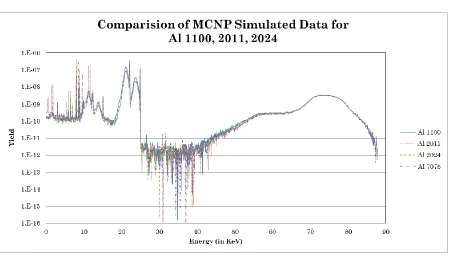
Figure 16 – MCNP Simulated Data ...41

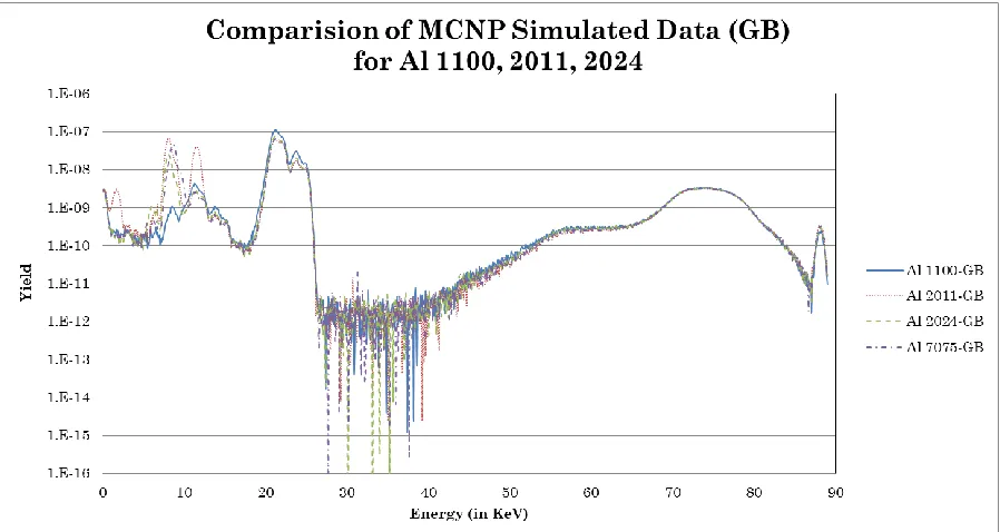
Figure 17 – MCNP Simulated Data (Gaussian Broadened) ...42

Figure 18 – Experimental Data with relevant peaks identified ...43

Figure 19 – Reduction of SS 302 data from 1024 channels to 128 channels ...45

Figure 20 – MCNP Data for Al-1100, Al-2011, Al-2024, and Al-7075 ...64

Figure 23 – Gaussian Broadened MCNP Data for 1100, 2011, 2024, and Al-7075 ...65

Figure 24 – Gaussian Broadened MCNP Data for 3003, 5052, 5086, and Al-5454 ...66

(15)

Figure 27 – Gaussian broadened MCNP Data for C101, C260, C260, C353, C464, and C510 ...67 Figure 28 – MCNP Data for Stainless Steel 302, 304, 316, 321, and 330 ...68 Figure 29 – MCNP Data for Stainless Steel 405, 430, 434, and 660 ...68 Figure 30 – Gaussian broadened MCNP Data for Stainless Steel 302, 304, 316, 321, and 330 ...69 Figure 31 – Gaussian broadened MCNP Data for Stainless Steel 405, 430, 434, and 660 ...69

(16)

Motivation and Background

The need and for fast and accurate elemental analysis is a problem faced by many different industries. In manufacturing processes, it is very useful to have an inline (or in situ) elemental detection system rather than batch testing. When inline elemental detection systems are integrated with quality controls, adjustments to manufacturing processes can be made in real time and with much less adverse effect on the final product. Many applications can benefit from an inline elemental analysis system, but a couple of examples will illustrate this point. In oil applications, it is important to determine the sodium, chlorine, and sulfur content while the oil is being pumped from the ground. These varying levels will ultimately determine how the oil is refined, what end products it makes, and what markets it is sold to. In coal applications there are rigorous EPA limits on sulfur concentrations that can be burned with coal. An inline system for determining the sulfur content of different veins would allow real-time classification and down mixing of over sulfurized coal tailings. This study looks at processes for real time classification of different metals in recycling applications. Since the 1970s, the amount of scrap metal reprocessed into new steel products has constantly risen [Pflaum]. Scrap metal represents a source of residual materials that may be undesirable in new products. Therefore careful classification of scrap will play an important factor in future manufacturing. The physical description (such as density, color, elasticity, ferrousity) can often be enough to broadly classify metals in categories such as steel, copper, aluminum, and brass. However, this description is often inadequate for distinguishing between highly similar metals such as stainless steel(SS) 304 and SS 316 which can be important in the re-smelting process because most stainless steels are not allowed to contain molybdenum (per ASTM A240) except for SS 316, which contains 2% – 3%. While there are methods for removing unwanted elements, it is more cost efficient and productive to begin with scrap of the same stock as that of the desired result.

(17)

ASTM E827-08]. The holy grail of element analysis is an in situ process that can provide near instantaneous and reliable results. For this requirement, spectroscopy is really the only method that offers a solution. Generation of spectroscopic data can occur in a multitude of ways, but it essentially works on the fundamental principle that the target materials are irradiated with either photons or particles inducing a nuclear or electron shell reaction. These reactions then emit characteristic photons that can be captured using a detector. Among the most popular methods are Energy Dispersive X-Ray Fluorescence (EDXRF), Neutron Activation Analysis (NAA), Prompt Gamma Neutron Activation Analysis (PGNAA), Laser Induced Breakdown Spectroscopy (LIBS), and Particle Induced X-Ray Emission (PIXE).

(18)

Figure 1 – Typical Features seen in a Gamma Spectra of Co-60

Monte Carlo Library Least Squares (MCLLS) developed by the Center for Engineering Applications of Radioisotopes (CEAR) at NC State offers a method for including all of the spectral information. This method has evolved through several iterations over the years; however, the general approach has always been to use Monte Carlo to generate a response (or spectrum) for each element given a particular source. These libraries are then

concatenated into a matrix A and can used to solve the equation

Ax = y (1.1)

where the vector

x

contains the elemental weights, and ycontains the experimental

spectra.

x

can be found by either using regression by calculating the covariance matrix,

T T

A Ax = A y (1.2)







T



-1 T

x = A A

A y

(1.3)

or through a non-linear search techniques to find the elemental weights by minimizing

(19)







1 2 3



min abs

x

...

x

_N







1



2



3

 

Ν







x

a

y

(1.4)

There are a couple of challenges one can encounter when using the MCLLS method.

Those include the covariance matrix T

A A

being ill-conditioned where there is a high

degree of covariance between libraries, generating negative weights for some of the elements, or having large residuals for areas of the spectra that are not well simulated.

The purpose of this work is to look at two additional techniques for analyzing spectroscopic data to overcome some of the issues with the MCLLS method. These techniques include Artificial Neural Networks and Partial Least Squares. Both methods present an opportunity to build mathematical models that not only describe the spectroscopic data of the calibrated samples, but will also help predict the properties within new samples. The first method implemented is the Artificial Neural Network (ANN). A Back Propagation Neural Network will be employed that uses the Levenberg-Marquardt algorithm for finding local minima within the solution, with a Levy Flight Random Walk process to handle the global minimization search. The second method is to use Partial Least Squares (PLS), a technique widely used in the field of chemometrics, to rotate the principle components (PCA) of the spectroscopic data such that a linear model can be formed to predict elemental weights.

(20)

Theory

Physical Interactions of X-rays

When dealing with thin, dense materials such as aluminum or steel, one of the most appropriate methods for generating spectra is through energy dispersive Xray fluorescence (EDXRF). X-ray spectroscopy is possible because it leverages the atomic structure of an element. The quantum model of the nucleus suggests that electrons orbit the nucleus in a series of shells (or states). Each shell exists at a discrete energy level and can be described by the principal quantum number (n), the angular momentum quantum number (l); the number of electrons that can exist within each shell and how they are arranged are described by these plus the magnetic quantum number (ml) and the electron spin quantum number (ms). In traditional chemistry, this would be equivalent to the n=1,2,3, and s, p, d, f orbitals notation seen in introductory chemistry texts (see Chang). Energy can be added to an atom by exciting an electron from one state (or shell) and elevating an electron to a higher energy shell. Atoms will always tend toward their most stable state and will shed excess energy to do so. An excited atom de-excites by emitting an X-ray as an electron drops from an elevated orbital state into a lower one. The energy of that X-ray is dictated by the conservation of energy and the difference between the final and initial energy of the host atom.

X X 



(2.1)

In X-ray spectroscopy applications, the principal quantum number is replaced by the convention of K, L, M,… radiations or emissions [Markowicz], where K represents the lowest energy state available to an electron. For example, a Kα emission is an X-ray that was born as a result of an electron transition from the L to the K level, K being the final state and α meaning from 1 level above. Likewise, an Lβ X-ray is a photon emitted from the N to L transition.

(21)

given photon (Kα of Cr for example) is correlated to the concentrations of all the other materials in the sample. X-ray spectroscopy in particular is unique because the photons

from elements of higher atomic number (or Z value) have the propensity for initiating

X-rays in lower Z materials [Sherman].

In 1955 Jacob Sherman published a paper that derived theoretical equations to explain the matrix effects seen in two- and three- element mixtures. Due to the complexity of this

charge he made a couple simplifications in his analysis. First, he limited the Z values of

the materials he was evaluating to 22 – 50 so that only Kα emissions would be present. Secondly, he assumed a monodirectional, monochromatic source. Lastly, he neglected tertiary effects (meaning anything beyond the second ionization was ignored). In 1978 Gardner and Doster found through the use of Monte Carlo simulation that ignoring tertiary effects was non-trivial when determining elemental concentrations [Gardner]. Given Sherman’s challenges, we can see that derivation of the theoretical yield for complex (anything beyond three elements) mixtures is impractical. Development of Monte Carlo simulation coupled with computational methods poses the best capability to tackle these challenges.

Detector Selection and Operation

Measurement of low energy photons (e.g. below 100KeV) requires that a detector have very little material between the measurement medium (e.g. crystal, gas, etc.) and the source; otherwise, the photons will attenuate in the structural material and never ionize the detection medium. As a result, it is necessary to use a detector that has a thin, low density window between the outer can material and the crystal. For practical purposes, the detector choice is limited to semi-conductor detectors such as low energy germanium detectors (LEGe), silicon lithium drifted detectors (SiLi), and silicon surface barrier detectors.

(22)

(23)

Table 1 – Select X-ray transition energies (in KeV)

Atomic # Element E(KeV) I% E(KeV) I% E(KeV) I% E(KeV) I% E(KeV) I% E(KeV) I% E(KeV) I% E(KeV) I%

5 B** 0.183 0.11 0.183 0.0560 ---- ---- ---- ---- ---- ---- ---- ---- ---- ---- ---- ----6 C* 0.277 0.19 0.277 0.0900 ---- ---- ---- ---- ---- ---- ---- ---- ---- ---- ---- ----7 N* 0.392 0.35 0.392 0.1700 ---- ---- ---- ---- ---- ---- ---- ---- ---- ---- ---- ----8 O* 0.525 0.55 0.525 0.2800 ---- ---- ---- ---- ---- ---- ---- ---- ---- ---- ---- ----12 Mg 1.254 2.00 1.254 1.0000 1.302 ???? ---- ---- ---- ---- ---- ---- ---- ---- ---- ----13 Al 1.488 2.60 1.487 1.2900 1.558 0.023 ---- ---- ---- ---- ---- ---- ---- ---- ---- ----14 Si 1.741 3.30 1.740 1.2900 1.836 0.084 ---- ---- ---- ---- ---- ---- ---- ---- ---- ----15 P 2.015 4.10 2.013 2.0400 2.141 0.184 ---- ---- ---- ---- ---- ---- ---- ---- ---- ----16 S 2.309 5.00 2.307 2.4900 2.468 0.345 ---- ---- ---- ---- ---- ---- ---- ---- ---- ----22 Ti 4.510 12.80 4.504 6.4000 4.934 2.140 ---- ---- 0.452 0.063 0.456 0.007 0.462 0.050 ---- ----23 V 4.952 14.50 4.944 7.3000 5.430 2.480 ---- ---- 0.511 0.120 0.514 0.013 0.522 0.096 ---- ----24 Cr 5.414 16.40 5.404 8.3000 5.947 2.780 ---- ---- 0.577 0.190 0.573 0.021 0.583 0.150 ---- ----25 Mn 5.898 18.30 5.886 9.3000 6.493 3.230 ---- ---- 0.640 0.260 0.639 0.029 0.651 0.200 ---- ----26 Fe 6.403 20.20 6.390 10.2000 7.060 3.630 ---- ---- 0.708 0.410 0.707 0.045 0.721 0.250 ---- ----28 Ni 7.478 24.00 7.460 12.2000 8.268 4.360 ---- ---- 0.854 0.500 0.853 0.056 0.871 0.340 ---- ----29 Cu 8.048 26.00 8.028 13.3000 8.907 4.690 ---- ---- 0.930 0.600 0.929 0.066 0.949 0.390 ---- ----30 Zn 8.639 28.00 8.616 14.3000 9.574 5.130 9.658 0.194 1.012 0.650 1.012 0.072 1.035 0.420 ---- ----33 As 10.543 32.70 10.508 16.8000 11.727 6.440 11.866 0.323 1.282 0.870 1.282 0.096 1.317 0.520 ---- ----34 Se 11.223 34.10 11.182 17.6000 12.497 6.880 12.655 1.250 1.380 0.980 1.379 0.108 1.420 0.580 ---- ----40 Zr 15.775 41.00 15.691 21.4000 17.667 9.320 17.971 1.330 2.043 1.660 2.040 0.190 2.125 0.900 2.219 0.012 41 Nb 16.616 41.80 16.521 21.9000 18.624 9.630 18.956 1.450 2.167 1.800 2.163 0.200 2.257 0.930 2.367 0.056 42 Mo 17.479 42.60 17.374 22.4000 19.607 10.020 19.967 1.880 2.294 1.900 2.290 0.210 2.395 1.000 2.521 0.100 47 Ag 22.163 45.60 21.991 24.2000 24.943 11.420 25.458 1.980 2.985 2.500 2.979 0.280 3.151 1.390 3.348 0.320 48 Cd 23.174 46.10 22.984 24.5000 26.095 11.680 26.644 2.190 3.134 2.600 3.128 0.290 3.317 1.510 3.529 0.380 50 Sn 25.271 45.70 25.044 24.7000 28.486 12.140 29.109 2.280 3.444 2.900 3.436 0.320 3.663 1.750 3.905 0.460 51 Sb 26.359 46.00 26.111 24.9000 29.726 12.290 30.388 2.370 3.605 3.000 3.596 0.340 3.844 1.840 4.101 0.520 52 Te 27.472 46.20 27.202 25.0000 30.996 12.470 31.699 3.910 3.770 3.200 3.760 0.360 4.030 1.960 4.302 0.580 82 Pb 74.970 46.20 72.807 27.7000 84.940 16.280 87.362 3.930 10.551 12.800 10.450 1.440 12.613 8.500 12.623 3.180 83 Bi 77.109 46.20 74.817 27.7000 87.351 16.290 89.849 0.000 10.839 13.200 10.731 1.480 13.023 8.800 12.979 3.280 Sources National Institute of Science and Technology: http://physics.nist.gov/PhysRefData/XrayTrans/Html/search.html Lawrence Berkeley National Laboratory: http://ie.lbl.gov/atomic/x2.pdf

Lβ-2

Kβ-2

Select X-ray Transition Energies (in KeV)

(24)

Review and Application of Artificial Neural Networks (ANNs)

Artificial Neural Networks (ANNs) are information processing models composed of densely interconnected computational units. They are modeled after highly parallelized biological computing systems such as the brain. These systems are well suited for problems such as pattern recognition, association, classification, and predictive modeling. There are a wide range of neural network models, each specialized to handle a certain set of the problems mentioned above. While this discussion will only focus on one type (the backpropagation network) an exhaustive discussion of artificial networks can be found in many of the referenced texts [Hagan, Freeman, etc.]. For the purposes of analyzing spectroscopic data, a neural network ideally suited for predictive modeling is needed. As in the case of spectroscopy, the goal is to use a spectrum of known data to predict the elemental composition of an unknown material. An overly simplified model would be:

ˆ

f(x) = y

(3.1)

where

x

represents a one column vector containing all of the spectroscopic data for one

sample, and

f( )



is the set of mathematical operations applied to

x

to produce an estimate

of the elemental weights which we call

y

ˆ

. The backpropagation network (BPN)

represents one such choice that allows this and will be discussed shortly.

Neural networks represent an ideal way for solving the “elemental analysis” problem for three reasons. The first is their adaptive programming, where processing models are learned by example rather than being pre-programmed (also referred to as supervised learning); this is especially useful when the nature of the problem is not well understood but there is abundant calibration data. The second is the ANN’s ability to model non-linear behavior. The “matrix effects” associated with the elemental analysis problem are by the very nature non-linear, and so it is apt to have a non-linear prediction model. Lastly, if structured properly, ANNs can ignore noise in strepitous environments.

(25)

nodes are layers, broken up into three distinct types – the input layer, the hidden layer, and the output layer – with each node interconnected with every other node in the succeeding layer as seen in Figure 2. A BPN can comprise a minimum of three layers, and in this study a three layer neural network is employed. In general, there is no restriction to the number of layers used; however computational costs and over fitting data to noise are considerations to be made when selecting the number of layers.

Figure 2 – Typical Structure of a Feed-Forward Neural Network

The interconnection between each node is called a weight and is synonymous with the term “synaptic gap.” The term aptly applies since the weights scale the amount each parent node contributes to the numerical value of each interconnecting child node.

In a simple three-layer feed-forward network, the input data are scaled by the weights and are summed at each node in the hidden layer. In order for the non-linear modelling capability to exist, these values are then normalized by a non-linear function such as the sigmoid or error function. After the hidden nodes take on these new values, they are fed

Input Layer Hidden Layer Output Layer

ni1

ni2

ni3

ni4

ni5

nh1

nh2

nh3

no1

no2

no3

no4

bi bh

Input Nodes

Hidden Nodes

Output Nodes

(26)

through a second set of weights and the process is repeated. The only difference is that the transformation function before the output layer is linear.

Figure 3 – Structure of Neural Net used in this study and its transformation functions.

A BPN is identical with respect to the feed-forward network approach but supplements it with a correction step. When building the model, the weights necessary for accurate prediction must be determined. Using calibrated data, we can feed X-ray spectra of known compositions into the network and then correct the weights based on the

calibrated response that we expect to see. The term backpropagation refers to the process

of taking the differences (or errors) between the ANN prediction and the true value, and then propagating corrections to the weights, beginning with the weights connected at the output layer, and then updating the next set of upstream weights, repeating the process until arrival at the input layer. Aside from a few rare cases, ANNs are not ideally suited for extrapolation but can handle interpolation quite well [Marsland]. As a result, training data that encompass the full range of possible data sets are required for optimum results.

(27)

Too many hidden nodes will mean that the solution will fit itself to the noise contained within the X-ray spectra, which is not desirable.

Since the author developed a specific purpose neural network program for this application, a formal mathematical description of the backpropagation network employed will be presented, along with the update methods and the various enhancements used for optimizing the global search that minimizes the errors between the model and the calibration data. Figure 3 and Figure 4 will serve as the reference for this network.

The Neural Network Algorithm

In an effort to be consistent in notation and treatment of vectors and matrices in both the Neural Network algorithm and the Partial Least Squares (PLS) algorithm, the following

convention will apply. All vectors(e.g.

x

) will be in bold lowercase font and should be

considered single column vectors. All matrices (e.g.

X

) will be in bold uppercase font.

x

represents the X-ray spectra of a single sample, and

y

is a vector containing the elemental

weights of that sample. The matrix

X

will contain the transposed vectors of

x

_i where

each row corresponds to the ith_{sample of a set of}_N_{samples and}_M_{energy bins. Likewise,}

the matrix

Y

will contain the transposed vectors of

y

i for N samples and L elements as

seen in Figure 4.

X =

Sample 3 ... ... ... ... Sample N

Sample 2 Sample 1

Y =

Sample 3 ... ... ... ... Sample N

(28)

In general, the samples are handled one at a time in BP Networks where X-ray spectroscopic data is fed to the input layer. The inputs are transformed by a set of weights and a bias node from the input layer to the hidden layer. These weights are initialized as random numbers at the outset of the algorithm.

To simplify the notation we can treat the weights as an I x H matrix

W

_H where I

represents the number of input nodes, and H represents the number of hidden nodes. In

essence, each row represents the contribution of the ith_{input node on each hidden node.}

At each node in the hidden layer, the weighted contributions from each input node are summed and added to a bias. These weights and bias are called the “hidden weights” and “hidden bias” respectively since they operate from the input to the hidden layer.

1 I h

j ij i h i

net w x b





 (3.2)

In matrix notation

h

b



h T

H

net = W x

(3.3)

All sums

 

h

net are then non-linearly transformed using either a Sigmoid function which

ranges from 0 to 1 or an Error function which ranges from -1 to 1. For this algorithm, the Sigmoid function was chosen since we would like the weights to keep the same sign during the transformation.

(29)

The Sigmoid function is

1

1 + e

-x and is defined as the operator

h j

f

, such that at each jth

node in the hidden layer, the superposition of weighted inputs is operated on in the following way.

 

1 _

_

1 exp

h h

j j h

j

f

net







(3.4)

The final values taken at the jth_{node of the hidden layer are then:}

 

h

j j j

h  f net (3.5)

The transformed data now become the input to the output layer. Another array of weights and bias node (“output weights” and “output bias” respectively) facilitates the summation of the hidden nodes into the output nodes.

1 H o

k jk j o j

net

w h

b







(3.6)

o

b



o T

O

net = W h

(3.7)

A final transformation takes place at the output layer. Since the non-linearity parameters have already been built in at the hidden layer, there is no need for a second

non-linear transformation. We can simply treat o

k

f

as a constant multiplier. For

simplicity,

f

_ko



1

. It has been shown that for two layer networks a sigmoid

transformation at the hidden layer and linear transformation at the output layer can approximate almost any function [Hornick].

   

o 1 o

k k k

f net   net (3.8)

 

o

k k k

(30)

Once final values have been calculated at the output layer, the output of the network is compared to the calibrated answers. If the requirements of the performance index have

not been met, then the differences are backpropagated through the weights

W

_O and then

H

W

and a new final answer is calculated.

Choice of performance index is limited to a couple of different options. Most common is

the sum of squared errors





2

SSE



yo , the mean square error

MSE

1 

y o



2

N







, and the



2_{test where}





2

y o

y









, where y is the expected value (calibrated value)

and o is the network’s output value. Any other choices are usually variations on these

(31)

Backpropagation using the Levenberg-Marquardt Algorithm

The Levenberg-Marquardt Algorithm was used to optimize the correction step in our backpropagation. This is a variation of Newton’s method which is a second- order method based on the second- order Taylor series where a quadratic approximation is made to

 

F x [Hagan]. The notation is where

g

is the gradient_F

 

x _, and

H

is the Hessian

of

x

2

 

F

 

 x .



1







 

1

2

k k k k k k k k

F

w

_



F

w

 

w

F

w

   

g

T

w

w H

T



w

(3.10)

Find the minimum by setting the derivative of the update equal to zero.

0

k  k k 

g H w (3.11)

1

k k k





w

 

H g

(3.12)

1 1

k k k k









w

H g

(3.13)

Finding and inverting the Hessian matrix can be extremely expensive in computational terms and may not be possible depending on how well conditioned the Hessian matrix is. The Levenberg Marquardt method approximates the Hessian Matrix using the Covariance matrix of the Jacobian (First order derivative).

2

2 

T



T

H

J J

S

H

J J

(3.14)





1

1 2

k k _k k



   T

w w J J g (3.15)

It may be found that T

J J

is not invertible as well. To make the approximated Hessian

invertible we simply need to make T

J J

positive definite by adding a symmetric positive

(32)



 

G

H

I

(3.16)









i  



i  i



i 



i



i 

 

i i

Gz H I z Hz z z z z (3.17)

Thus the eigenvectors of G remain the same with only the magnitude of the eigenvalues

changing.





1

2

k k k

k















T







w

J J

I

g

(3.18)

If we choose the performance index to be the sum of squares, then:

2 1 ( ) N T i i F e  





w e e (3.19)

Where e_i  y_i o_i then the gradient is:

1

( )

2

N

i

k j i

i j

e

F

e

dw





 









T

g

w

J e

(3.20)

The Jacobian represents the first order derivative of the error with respect to the weights.

s



J

[

𝜕𝑒1

𝜕𝑤𝑜,1,1 ⋯

𝜕𝑒1

𝜕𝑤𝑜,𝐻,𝑂

𝜕𝑒2

𝜕𝑤𝑜,1,1 ⋯

𝜕𝑒2

𝜕𝑒1

𝜕𝑤ℎ,1,1 ⋯

𝜕𝑒1

𝜕𝑤ℎ,𝐼,𝐻

𝜕𝑒2

𝜕𝑤ℎ,1,1 ⋯

𝜕𝑒1 𝜕𝑤ℎ,𝐼,𝐻 𝜕𝑒1 𝜕𝑏𝑜 𝜕𝑒1 𝜕𝑏ℎ 𝜕𝑒2 𝜕𝑏𝑜 𝜕𝑒2 𝜕𝑏ℎ ⋮ ⋮ ⋮ ⋮ ⋮ ⋮ 𝜕𝑒𝑂

𝜕𝑤𝑜,1,1 ⋯

𝜕𝑒𝑂

𝜕𝑤ℎ,1,1 ⋯

𝜕𝑒𝑂 𝜕𝑤ℎ,𝐼,𝐻 𝜕𝑒𝑂 𝜕𝑏𝑜 𝜕𝑒𝑂 𝜕𝑏ℎ] (3.21)

To evaluate the SSE across all samples at the same time, the Jacobian becomes the concatenation of all the Jacobian matrices of each sample.

1 2 S              J J J J (3.22)

(33)

k k k

e

 

y

o

(3.23)

The derivative of the error with respect to the output weights is

 

o k

k k

o o o

jk k jk

net

e

o

w

net

w





 



(3.24)

Where the partial derivatives for the output weights are simply:

 

k 1

o k o net  _  (3.25)





1 o _H k o

jk j j

o o

j

jk jk

net

w h h

w w 

 _

 

 



(3.26)

The derivative of the error with respect to the output bias is

 

o k

k k

o o o

k

net

e o

b net b



 

  

   (3.27)

 

1

o k o

net

b



 



(3.28)

1 k o e b   

 (3.29)

Since there is no correction data available for the hidden layer values, we must backpropagate the errors contained in the output layer to the hidden layer weights using the chain rule.

 

o h

k j j

k k

h o h h

ij k j j ij

net h net

e o

w net h net w

  

 

  

     (3.30)

 

k

1

(34)

 

_



_



_

2

exp

1 exp

h j j h _h j _j

net

h

net

_net









_

_

(3.33)

 

1

h _I

j h

ij i i

h h

i ij ij net

w x x

w w 

 _

 

 



(3.34)













2

exp

1 exp

h j o k jk i h h ij j

net

e

w

x

w

_net







 



_

_

(3.35)

Repeating the same steps above for the hidden bias, the final partial derivative is













2

1

exp

1 exp

h H j o k jk h h j j

net

e

w

b



_net















_

_

(3.36)

The update method can now be generalized to the following: If all of the weights and

biases from every layer are arranged into one column array

w

, then





1

k k

k















T







T

w

J J

I

J e

(3.37)

The power in the Levenberg Marquardt method is in the selection of



. When



is large

the update procedure is slow, so if the corrections implemented reduce the SSE, then we

would like to scale



down so that that it will reach the minimum faster. An arbitrary

constant can be used, but a common selection is c10, where

 



c

. However, if the

selection of



results in an increase in the SSE, then it means the step size is too large

(35)

Figure 7 – Flow Diagram of the ANN Algorithm Pre-process input data

Generate random weights WH=WIxH

WO=WHxO

Calculate Summations on hidden layer neth=WHTx

Apply Sigmoid function For j=1:H; hj=1/(1 + exp(-nethj))

Calculate Summations on output layer neto=WOTh

Apply Linear function For k=1:K; ok=1*(-netok))

Calculate Errors E = (y – o)2

Use Levenberg Marquardt to find new weights LM Convergence

Criteria Met?

Update weights WH= WH + ΔWH W_O= W_O + ΔW_O

STOP

Yes

(36)

Review and Application of Partial Least Squares Regression

Partial Least Squares (PLS) is a linear regression technique developed by H. Wold in the 1960s. It is used to maximize the correlation between the explanatory variables in one data set and the response variables in another data set. In model building, it is often helpful to functionalize explanatory variables so that the response variables can be predicted.

Y = f(X) (4.1)

In PLS Regression,

X

and

Y

can be considered the composition of two matrices where the

decompositions are a set of orthogonal factors T

X

X = TP + R

and

Y = UQ + R

T _Y, where

T

and

U

are the scores,

P

and

Q

the loadings, andR_XandRYthe residuals. Principal

Component Analysis (PCA), a forbearer to PLS, uses the latent structure of these matrices

to find a set of scores and loadings that best describes the variation in the

X

and

Y

data

blocks. PLS differs only in the sense in that it also seeks regression coefficients (the

diagonal entries of

B

) such that the combination of scores, loadings, and regression

coefficients best use the variation in

X

to explain the variation in

Y

[Bro].

In gamma ray and X-ray spectroscopy, this method can be leveraged as long as there are

an adequate number of verifiable samples. With known

X

and

Y

data blocks, the scores,

loadings, and regression coefficients can be generated and then used to predict the response variables from new samples. Equation 4.1 can be reformulated to project the

scores of

X

onto the loadings of

Y

through a set of regression coefficients

B

.

ˆ T

Y = TBQ (4.2)

Where Yˆ is an estimate of

Y

.

The PLS Algorithm

In this description of the PLS Algorithm, it will be implied that the row vectors of

X

and

Y

will represent each individual sample. The column vectors in

X

will correspond to a

predictor variable (i.e. channel number or energy). The column vectors in

Y

are the

(37)

We begin by scaling and centering the

X

and

Y

data blocks by converting each matrix

element into a Z-score. The purpose of this is to allow data with different magnitudes and units to be put on equal footing. Each column vector contains all the values for one variable; therefore, the mean and standard deviation are calculated for each. Hence the

variations in the elements of

X

and

Y

are normalized and converted into units of per

standard deviation. To avoid confusion, we define the matrices

E

and

F

as the scaled and

centered data of

X

and

Y

.

ij j ij

j

x









(4.3)

ik k ik

k y

y







 (4.4)

Scaled_&_Centered

E = X

F = Y

(4.5)

To decompose

E

to

F

into its respective scores and loadings, an iterative approach is used

to determine the vectors for

T

,

P

,

U

,and

Q

one component at a time. (Note the terms

component and latent variable are used interchangeably). If the number of components

chosen is equal to the rank of

X

, then all of the variation of

X

is explained in the

component scores (Bro). This is often undesirable, since

X

often contains noise that limits

the full utilization of

X

from being the best predictor. An optimization method for

choosing the right number of components will be discussed later, but is an important part

of the PLS model. For the first iteration of each component, the vector

u

is populated

with random numbers.

T

T 2

E u

w =

E u

(4.6)

2

Ew

t =

(38)

2

Ft

q =

Ft

(4.8)

u = Fq (4.9)

Perform the above iteration until

t

converges to the desired convergence criteria. The

vector

p

and regression coefficient

b

are then calculated so that the contribution of a

particular component can be deducted from the

Ε

and

F

matrices.

T

2

E t

p =

t

(4.10)

b



T T T 2

t u

=

t u

t t

(4.11)

T

E = E - tp (4.12)

b

T

F = F - tq

(4.13)

To determine how much a particular component explains

X

and

Y

, the following

relations can be used, where SSE and SSF denote the sum of squares for

E

and

F

respectively, and LVE and LVF represent the amount each Latent Variable explains

E

and

F

respectively.

2 E E F F

LV

SS

b

LV

SS



T

p p

(4.14)





 





 

2 2 2 2

E ij ij

F ik ik

SS

e

SS

f













(4.15)

As components are generated, they will always explain a decreasing amount of the parent

matrices. The vectors

t

,

u

,

w

,

q

, and

p

are stored as the column vectors of

T

,

U

,

W

,

Q

,

(39)

as the diagonal entries of

B

. This process is repeated until

E

and

F

are nearly

equivalent to the

NULL

matrix.

Using equation 4.16, the optimum number of components for the model is where the

residuals between

F

and Fˆare minimized.

ˆ T

F = TBQ (4.16)



ˆ



optimum

LV

= min abs F - F



_

_i



_

(4.17)

For convenience when evaluating unknown data sets, the t scores and weighting factors call be lumped into one term.

ˆ

Unk Unk PLS

F = E B (4.18)

† T

PLS

B

= P BQ

(4.19)

Where †

P

is the Penrose Moore inverse of

P

.

Keep in mind that ij j

ij

j

x

e









E

which means that the results of Fˆ are not direct

evaluations of Yˆ . To functionalize

B

_PLS into terms of

X

_Cal and Y_Cal, a multiple linear

regression (MLR) must be completed on each vector inYˆ_Cal. Completion of the PLS

Algorithm determines the optimal number of latent variables that explains the

X

and

Y

data. Assuming that the optimum number of latent variables is L, the mulitvariate

regression that occurs can be expressed as:

1

ˆ_i a_i b_i c_i ₂ ... m_i _L

y = + v v v (4.20)

j j PLS

v = x B

(4.21)

The goal is now to find the set of coefficients



a_i...l_i



such that



y_iyˆ_i



2 is minimized. To

(40)

The first normal equation is:

1 2

1 1 1 1

...

n n n n

jk j j jL

j j j j

y an b x c x m x

   

    



(4.22)

The second normal equation is:

1 1 1 1 1 2 1

1 1 1 1 1

...

n n n n n

j jk j j j j j j jL

j j j j j

x

y

a

x

b

x

c

x

m

x

    













 





(4.23)

The third normal equation is:

2 2 2 1 2 2 2

1 1 1 1 1

...

n n n n n

j jk j j j j j j jL

j j j j j

x

y

a

x

b

x

c

x

m

x

    













 





(4.24)

This pattern is repeated through to the Mth_{normal equation:}

2 2 1 2 2

1 1 1 1 1

...

n n n n n

jL jk L L j L j jL jL

j j j j j

x

y

a

x

b

x

c

x

m

x

    













 





(4.25)

With M equations in hand, we can solve for the coefficients



a m

...



. Arranging the

coefficients



b m...



into an N by L matrix B_SCL(where N is the number of samples), the Yˆ

estimate can be directly solved for:

ˆ

PLS_NEW

Y = XB

+ A

(4.26)

PLS_NEW PLS MLR

B

= B

B

(4.27)

1 1 1

...

L L L

a









 











N×L

A

(4.28)

(41)

Simulation Methods and Design

To supplement the experimental data, simulated X-ray spectra were generated using the Monte Carlo Method. The Monte Carlo approach simulates the random walk of a particle by sampling the probability density functions (PDF) for each phase space the particle enters. Since photon transport and its interactions with matter is viewed as a stochastic process, it follows that this sampling method is well suited for this application.

MCNP 5, a General Purpose Monte Carlo Neutron Transport Code developed by the Los Alamos National Laboratory with origins going back to the Manhattan Project, was the code chosen to generate the spectra. MCNP itself is considered one of the gold standards in general purpose Monte Carlo (Along with Geant4 and others). The version MCNP 5 was observed to have significantly better figures of merit over MCNP 6, hence that was the software chosen.

MCNP 5 uses two different types of treatments for photon physics and can be specified by the user. The simple physics model accounts for incoherent (Compton) scattering, photoelectric absorption, and pair production and is well suited for higher energy physics problems. The detailed physics model additionally includes coherent (Thomson) scattering, fluorescent photon emission, auger electron transport, plus bremsstrahlung. Detailed mathematical descriptions of these transport processes can be found in the

MCNP User Manual Vol I. The detailed physics model was chosen for fluorescent emission and auger electron physics which is critical for this particular application. Figure 8 shows the geometry of the simulated experiment using the geometry visualizer VISED.

(42)

For this particular simulation, the probability of an X-ray being emitted towards the target, hitting the material, resulting in a new photon directed towards the detector and ultimately being absorbed was relatively small. For this reason a number of variance reduction techniques had to be employed in order to obtain statistically viable results. These variance reduction techniques include: direction biasing, collision forcing (aka implicit capture), particle splitting, and weight cutoff limits with Russian roulette.

Figure 8 – MCNP Model of a LEGe Detector, Metal Target, Cd-109 X-ray Source, and Lead Collimator

Target

LEGe Detector

Xray Source

(43)

To demonstrate how this works, the initial particle is emitted from a 60° cone that lies centered on the x axis and directed towards the target. The base weight is updated with the probability that an isotropic source would have emitted a photon in this direction in the first place which is equal to the fraction of the solid angle over the unit sphere or

4

w





 . If the photon passes the surface of the target, a collision is forced and is sampled

from the PDF given in equation 5.1





1 exp _td (5.1)

The distance a particle travels before interacting can be directly sampled from a uniform distribution by integrating equation 5.1 and normalizing it:













1

ln 1 1 exp _t

t

x  



 d

 (5.2)

where

x

is the distance traveled into the material,



t is the total cross section,

d

is the

cord length of the material along the vector of travel, and where  is a uniformly

distributed random number on the range [0,1). The base weight is subsequently updated

tow  w



1 exp



_td



.

If any subsequent particles resulting from this interaction are directed towards the detector face, then the information yield from that particle is maximized by splitting it as

it crosses the crystal surface. The base weight for each split photon becomes ww n

where

n

is the number of split particles. Collision forcing is applied again inside the

(44)

reduction techniques described above, and still allow final particles to be counted towards the tally. Any further weight reduction would suggest that the particle was on a track not likely to enter the detector. After the weight cutoff limit is reached, Russian roulette is performed in such a way that the mean of each tally is preserved. Russian roulette can be summed up in this simple algorithm



Base L imit

L imit

Base L imit

I f w

< w

φ= rand[0,1)

I fφ < w

t hen

w

:= w

Else

Par t icle is k illed

End

(45)

Table 2 – Metals used in the simulation

Metal Samples

used in Simulation

Material

ASTM

Standard

Aluminum

1100

2024

3003

5086

5454

6061

6063

6101

7075

Steel

302

304

316

321

405

430

434

660 Copper/Brass/

C101

Bronze

C110

C122

C260

C353

C464

C510

(46)

Experimental Methods and Design

Experimental Design

An experiment was developed to test the ANN and PLS methods using experimental data rather than simulated data. Figure 10 shows a block diagram of the experimental set up, which includes the following pieces of equipment:

Equipment:

1. Various Al, SS, and Cu Metal Samples

2. Low Energy Germanium Detector (LEGe) - Canberra GL1515R with:

a. Built in pre-amplifier (Canberra 2002CPSL)

b. Cryostat Configuration 7500SL

c. Dewar Model DWR-30

3. HV Supply (Ortec 459)

4. Amplifier (Canberra 2026)

5. Oscilloscope (Tektronix TDS 2012)

6. 750 μCi Cd109_Source

7. ORTEC Easy-MCA-8K

8. Sample/Source holder

9. Lead Collimator

Data Collection Software:

1. ORTEC GammaVision-32 v7.01

Figure 10 – Block Diagram of the Experimental Setup

LEGe Detector Pre-Amp Amplifier

Oscilloscope

ORTEC Easy-MCA-8K 2000 HV

Power Supply _{Pre-Amp Power}

Cd109 Source

(47)

Table 3 – Settings for the Experimental Equipment

Power Supply

Amplifier Settings

Voltage

Gain

Shaping Time

Pulse Mode

-2000V

100 X .5

6μs

Uni-Polar

Each sample is laid on the wooden frame at a 45° angle above the LEGe Detector. On the opposing side of the frame, a collimated Cd109 source is used to irradiate the sample as seen in Figure 11 and Figure 12.

(48)

Figure 12 – Side view of detector, target, and collimator

(49)

(50)

The detector was calibrated and its resolution characterized using two different sources,

the first being Cd109_{and the second source being Am}241_{. The two sources emit a number}

of different gamma and X-rays as seen in Table 4.

Table 4 – Characteristic Xray and gamma ray emissions for Cd109_{and Am}241 Characteristic X-Ray and



-Ray Emissions (Partial List)

Radioisotope Energy(KeV) Yield(%) _CalibrationUsed for Type

Cd

109

2.978

4.5 No

L1

3.151

2.6 No

L1

21.990

29.5 No

K2

22.163

55.7 No

K1

24.912

4.76 No

K3

24.943

9.2 No

K1

25.455

2.3 Yes

K2

88.04

3.61 Yes



Am

241

13.761

1.07 No

L2

13.946

9.6 No

L1

16.816

2.5 No

L2

17.061

1.5 No

L4

17.751

5.78 No

L1

17.992

1.37 No

L3

20.784

1.39 No

L1

26.3448

2.40 No



59.5412

35.9 Yes



Due to the number of convolved peaks only three peaks could be found which correlated to a discrete energy. Those included the 26.3448 and 59.5412 KeV gamma rays from

Am241_{and the 88.04 KeV photon from Cd}109_{. These three energy peaks were used to}

characterize the resolution of the detector. For calibration purposes the number of peaks

used was expanded to include the 13.761/13.946 convolved peak from Am241_{and the}

(51)

The following model as seen in equation 6.1 was used to fit these data points and collect the necessary parameters for the GEB card in MCNP. Although the experiment and first round of simulations were independent of each other (meaning the simulation was not meant to replicate the experiment), the GEB parameters did provide a means to add noise to the simulated data that was consistent with the experiment and could be used in a second round of simulations that does replicate the experiment.

 



2



sqrt

fwhm E  B E C E A (6.1)

A non-linear search was performed to find the coefficients A, B, and C.

Table 5 – Gaussian broadening parameters

FWHM(E) Coefficients

A

7.003E-4

B

9.931E-5

C

265

(52)

Table 6 – Metals used in the experiment

Metal Samples

used in Experiment

Material

ASTM

Standard

Aluminum

1100

2024

2036

3003

5086

5454

6061

6063

6101

7050

7075

Steel

302

304

316

321

430 A569

A653

Copper/Brass/

C101

Bronze

C110

(53)

(54)

Uncertainty Analysis and Error Quantification

To determine the error bounds of the solutions proposed by the ANN and PLS algorithms the uncertainty in the Spectroscopic data (the X block), the uncertainty in our calibration data (the Y block), and the error in the predictions (the Yest Block) must be considered. Adding to this complexity is that when building our model we will also have residual

error, meaning that if X_Cal, Y_Cal are the original data blocks used to determine the model

parameters and

X

_Cal is plugged into the model, it does not necessarily mean that Y_Calis

retrieved, but rather an estimate of Y_Calis calculated called Yˆ_Cal





ˆ

f

X

_Cal



Y

_Cal



Y

_Cal (6.2)



ˆ



abs

 

residual Cal

E Y Y (6.3)

Uncertainty in the Spectroscopic Data

Counting statistics in the nuclear field can be characterized as a Poisson distributed process which is a special case of the Binomial distribution, where the probability of an event approaches zero while the total number of trials approaches infinity. As a result,

the expected number of counts in the ith_{given channel can be considered to have a mean}

equal to the number of observed counts with a standard deviation equal to the square root of observed counts. [Knoll].

expected observed observed

i i i

C



C



C

(6.4)

Residual Error

As mentioned before the residual error is simply the amount calculated in equation 7.2. In this study, the model error was the largest source of error and as a result in the uncertainty in the Y data could be ignored, since it is much smaller than the model error.





residual Y

A Comparative Analysis of Partial Least Squares (PLS) Regression and Artificial Neural Network (ANN) Methods for Determining Elemental Weights in Sheet Metal.

ABSTRACT

Dedication

Biography

Acknowledgements

Table of Contents

List of Tables

List of Figures

Motivation and Background

x

x









x = A A

A y









min abs

x

x

x

...

x









 







a

a

a

a

y

A A

Theory



Review and Application of Artificial Neural Networks (ANNs)

ˆ

f(x) = y

x

f( )



x

y

ˆ

x

X

x

y

X

x

Y

y

W



b



net = W x

 

1

1

+ e

f

 

1





1 exp

f

net

net





_

_