Abstract
Alldredge, Mathew W. Avian point count surveys: Estimating components of the
detection process. (Under the direction of Kenneth H. Pollock and Theodore R. Simons) Point count surveys of birds are commonly used to provide indices of abundance or, in some cases, estimates of true abundance. The most common use of point counts is to provide an index of population abundance or relative abundance. To make spatial or temporal comparisons valid using this type of count requires the very restrictive
assumption of equal detection probability for the comparisons being made.
We developed a multiple-independent observer approach to estimating abundance for point count surveys as a modification of the primary-secondary observer approach. This approach uses standard capture-recapture models, including models of inherent individual heterogeneity in detection probabilities and models using individual covariates to account for observable heterogeneity in detection probabilities. Two-observer models provided negatively biased estimates because they do not account for individual
heterogeneity in detection probabilities. Models accounting for individual heterogeneity are always selected as the most parsimonious models for this data type.
We also developed a time of detection approach for estimating avian abundance when birds are detected aurally, which is a modification of the time of removal approach. This approach requires collecting detection histories of individual birds in consecutive time intervals and modeling the detection process using a capture-recapture framework. This approach incorporates both the probability a bird is available for detection and the probability of detection given availability. Analyses presented demonstrate the
We recommend time of detection point count surveys be designed with four or more equal intervals.
We also present a multiple species modeling strategy since many point count surveys collect data on multiple species and present the approach for distance sampling, multiple observer, and time of detection approaches. The purpose of using a multiple species modeling approach is to obtain more parsimonious models by exploiting similarities in the detection process among species. We present a method for defining species groups which leads to an a priori set of species groups and associated candidate models. Multiple species models worked well and in many cases gave more
parsimonious models than a species specific modeling approach, especially for the multiple-observer and time of detection approaches. Parameter estimates for multiple species models are more precise than single species models. We recommend this approach for all situations where data on multiple species is collected.
as count lengths get short. We recommend this approach when “snapshot” type counts are necessary.
To my family:
Biography
I grew up in the mountains of Colorado and Wyoming. My free time was always spent outside, skiing, hiking, fishing, hunting and otherwise goofing off in the mountains. I learned to enjoy wildlife at an early age and am always at my best when interacting with it and trying to learn and understand how all the pieces fit together. I also had the
opportunity of growing up and interacting with several wildlife biologists, including my father, and gained many valuable experiences helping with their projects.
Seeing the stress and bureaucracy involved with wildlife research and management I thought it might be wise to follow a different career path and let my wildlife interests occupy my free time instead of my profession. I completed an undergraduate degree in mechanical engineering in 1994 and then quickly decided that office life was not for me. I started taking wildlife courses at Colorado State University and worked on a few fish projects. Then I took a job working on a grizzly bear study in Wyoming. While camped at the foot of the Tetons trapping and tracking bears I gained the experience of a lifetime which solidified my career path.
I attended the University of Idaho for my Master’s of Science in Wildlife Resources. My master’s project examined elk habitat and nutritional relationships on industrial timber lands. My advisor, Jim Peek, taught me more about wildlife and ecosystems than I could ever learn from books.
Carolina State University. In 2002 I completed a master’s in biomathematics. Having an interest in population dynamics and modeling as well, I decided to co-major in
Acknowledgements
First I would like to thank my graduate committee for their support and advice they provided me. Ken Pollock provided me many opportunities to work on a variety of projects during my four years at NCSU and helped me develop a broad background in sampling wildlife populations. Ted Simons brought me on board the “Bird Radio” project and continuously advised me on the intricacies of point counts. Jim Nichols not only was willing to fly down to NCSU for committee meetings but also helped me think through the sampling and modeling issues I proposed and dealt with many questions about model results (the ominous c-hat). Always remember to “think hard” about something. Cavell Brownie helped and encouraged me on the statistical development of my research and always had ideas on improving my techniques. Jim Gilliam, another great thinker, always looked for applications to more general questions and challenged my model assumptions. I owe the singing time model of Chapter 5 to this. I would also like to thank Jaime Collazo for his assistance on this project.
This project was funded by the U.S. Geological Survey and the National Park Service.
I also appreciate all of the field work that went before me. Without the
accessibility of these data sets for example analyses of my methods my thesis would have been little more than statistical rambling. I would thank each field technician by name but I know them only by the initials appearing on the data sheets.
Table of Contents
LIST OF TABLES
LIST OF FIGURES
CHAPTER 1
INTRODUCTION
CHAPTER 2
ESTIMATING DETECTION PROBABILITIES FROM MULTIPLE
OBSERVER POINT COUNTS
ABSTRACT
INTRODUCTION
METHODS
Field Methods
Primary-Secondary Observer Model
Two independent observer model
Four or more independent observer models
Analyses
Comparison of Dependent and Independent Observer Models
Field data
Two independent observer examples
Four independent observer examples
Heterogeneity simulations
Page
xii
xvii
1
12
13
14
17
17
19
20
23
26
26
27
28
29
RESULTS
Comparison of dependent and independent observer models
Two independent observer examples
Four independent observer examples
Heterogeneity simulations
DISCUSSION
Field application
Example analyses
RECOMMENDATIONS
LITERATURE CITED
APPENDIX 1: Common and scientific names for the “Warbler” and “Vireo” species groups used for analysis.
CHAPTER 3
TIME OF DETECTION METHOD FOR ESTIMATING ABUNDANCE FROM POINT COUNT SURVEYS
ABSTRACT
INTRODUCTION
METHODS
Field Methods
Detection process
Approach and candidate models
General form of model
Models without heterogeneity
Heterogeneity models
Covariates
FIELD TRIALS
RESULTS
Three Interval Data Set
Four Interval Data Set
DISCUSSION
RECOMMENDATIONS
LITERATURE CITED
CHAPTER 4
MULTIPLE SPECIES ANALYSIS OF POINT COUNT DATA: A MORE PARSIMONIOUS MODELING FRAMEWORK
ABSTRACT
INTRODUCTION
METHODS
Field Methods
Defining Species Groups
Model Selection
Multiple Species Modeling Strategy
ESTIMATION METHODS AND CANDIDATE MODELS
Distance
Time of Detection
Multiple Observers
FIELD TRIALS
Species Groups
Distance Analysis
Time of Detection Analysis
Multiple Observer Analysis
RESULTS
Species Groups
Distance
Time of Detection
Independent Observer
DISCUSSION
RECOMMENDATIONS
LITERATURE CITED
CHAPTER 5
MODELING THE AVAILABILITY PROCESS FOR POINT COUNT
SURVEYS USING AUXILIARY DATA
ABSTRACT
INTRODUCTION
METHODS
Field Methods
Availability Assuming Homogeneous Singing Rates
Availability Assuming Heterogeneous Singing Rates
Estimating Variance and Confidence Intervals
Availability Using Singing Times
ANALYSIS OF FIELD DATA
RESULTS
Singing Rate Models
Singing Time Model
DISCUSSION
RECOMMENDATIONS
LITERATURE CITED
CHAPTER 6
EXECUTIVE SUMMARY
INTRODUCTION
Chapter 2:ESTIMATING DETECTION PROBABILITIES FROM MULTIPLE
OBSERVER POINT COUNTS
Objectives
Implications and Findings
Chapter 3: TIME OF DETECTION METHOD FOR ESTIMATING ABUNDANCE FROM POINT COUNT SURVEYS
Objectives
Implications and Findings
Chapter 4:MULTIPLE SPECIES ANALYSIS OF POINT COUNT DATA: A
MORE PARSIMONIOUS MODELING FRAMEWORK
Objectives
Implications and Findings
Chapter 5:MODELING THE AVAILABILITY PROCESS FOR POINT
COUNT SURVEYS USING AUXILIARY DATA
Objectives
Implications and Findings
GENERAL CONCLUSIONS
APPENDIX 2: SURVIV CODE: Time of Detection Analysis
Single Species Code
Multiple Species Code (4 species example)
APPENDIX 3: SINGING TIME PROGRAMS
MATLAB Code for Singing Time Analysis
Screen Layout for Singing Time Data Collection
200
201
202
204
205
207
216
217
List of Tables
Chapter 2: ESTIMATING DETECTION PROBABILITIES FROM MULTIPLE OBSERVER POINT COUNTS
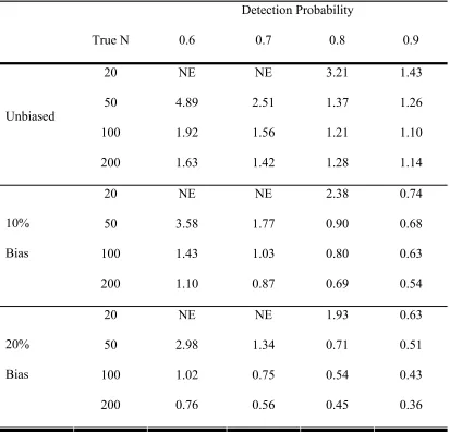
Table 1: Comparison of the dependent-observer approach to the independent- observer approach using simulations of 1,000 data sets for each population size, detectability and method. The unbiased scenario is the ratio of the SE of the dependent-observer method to the SE of the independent-observer method. The biased scenario represents 10% and 20% of the observations in the independent-observer data being dependent on the first observer and compares the ratio of the SE of the dependent-observer method to the MSE1/2 for the independent observer method.
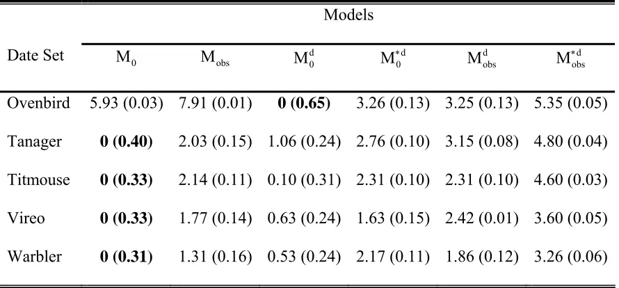
Table 2: Model selection for the two-independent observer examples giving the
∆AICc values for all 6 candidate models. The smaller ∆AICc values indicate a more parsimonious model with 0 indicating the selected model. AICc weights in parentheses.
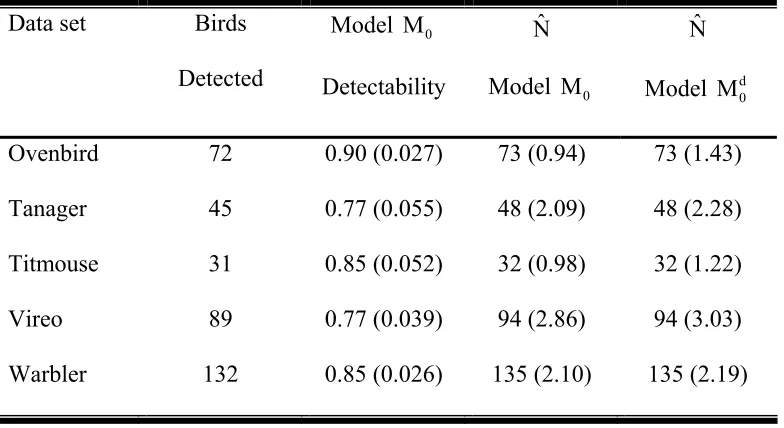
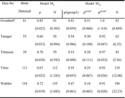
Table 3: Abundance estimates (N) for the two-independent observer examples. Birds detected are the totals between the two observers. Model M0 was selected as the most parsimonious for all data sets except the Ovenbird.
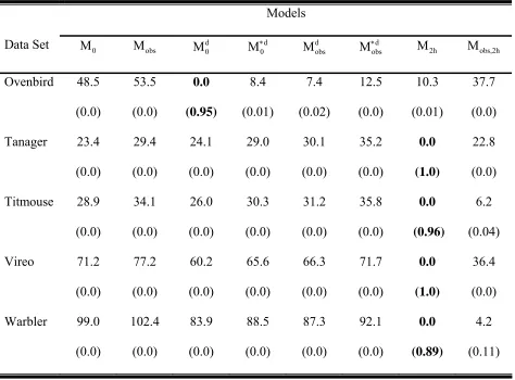
Table 4: Model selection for the four-independent observer examples giving the
∆AICc values for all 8 candidate models. Model M and model 2h Mobs,2h are based on 2 point mixture models of heterogeneity. The smaller ∆AICc values indicate a more parsimonious model with 0 indicating the selected model. AICc weights are in parentheses.
Table 5: Abundance estimates (N) for the four-independent observer examples. Birds detected are the totals among the four observers. Detection
probabilities are given by p for model M and p0 group1 and pgroup2 for model
2h
M . The proportion of the population in group 1 is given by pr(group1). Standard errors are in parentheses.
49
50
51
52
Table 6: Abundance estimates for four-observer and two-observer methods and a single observer count from simulated heterogeneous data from three- and two-point mixture distributions. For the three-point mixture distribution 20% of the population had detection probability 1, 60% had detection probability 0.75, and the remaining 20% had three different levels (low = 0.5, moderate = 0.3, and high =0.1) of detection probabilities. For the two-point mixture distribution half the population had high detection probability (p=0.9) and the other half low detection probability (p=0.1 or p=0.2), which gave capture histories similar to those observed in the
“Warbler” data set.
Chapter 3: TIME OF DETECTION METHOD FOR ESTIMATING ABUNDANCE FROM POINT COUNT SURVEYS
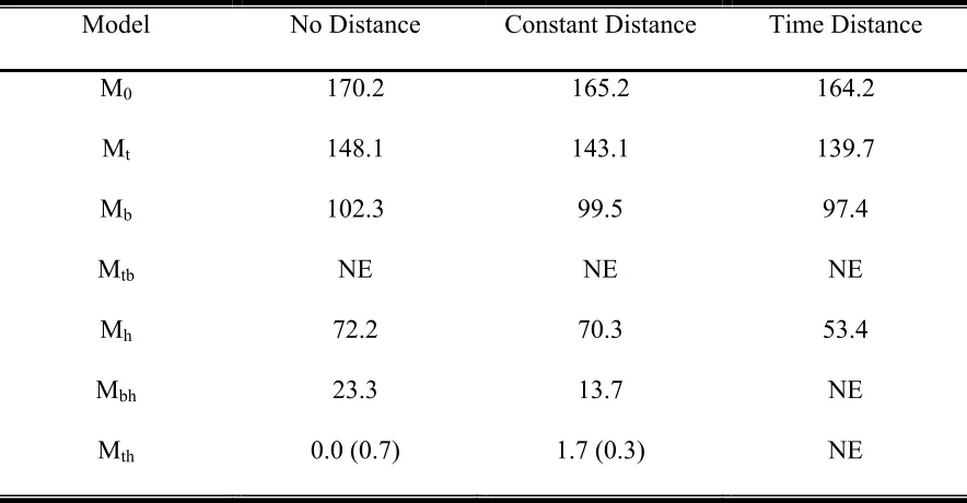
Table 1: ∆AICc values for the 11 time of detection models fit to each data set.
∆AICc = 0.0 for the most parsimonious model for each data set. ∆AICc weights (in parentheses) indicate the strength of the evidence for a given model compared to the other models (the larger number indicates more
evidence for that model).
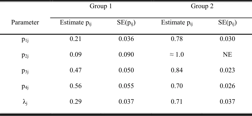
Table 2. Parameter estimates from the selected model for the 3 interval point count data sets. λ1 is the proportion of the population that is in group 1. Detection probability (pij) is the probability of detecting an individual from group j in interval i. The detection probabilities for group 2 (pt2)
were fixed. Standard errors in parentheses.
Table 3: ∆AICc values for the four time interval Thrasher data set. A value of 0.0 indicates the most parsimonious model. ∆AICc weight is in parentheses where weight is nonzero. NE indicates models that were not included because of unreasonable parameter estimates.
Table 4: Estimated detection probabilities pij, probability of group occurrence λj and standard errors for interval i and group j of the four time interval Thrasher data set based on model Mth. Standard error for group two and time interval two is not estimable.
54
95
96
97
Chapter 4: MULTIPLE SPECIES ANALYSIS OF POINT COUNT DATA: A MORE PARSIMONIOUS MODELING FRAMEWORK
Table 1: Number of parameters in candidate models for the time of detection method with t time periods and s different species. Behavior models assume a single behavioral response and heterogeneity models are based on a 2 point mixture. Models with a superscript +spp indicate an additive effect between observers and species and models with a superscript *spp indicate an interaction effect between observers and species. Models with superscript part indicate those that have similar detection probabilities between species but different probabilities of being in the first group. An additional parameter is required for each model to estimate abundance.
Table 2: Number of parameters in candidate model for the multiple observer method using t observers, s species and heterogeneity models based on a 2 point mixture model. Models with superscript part indicate those that have similar detection probabilities between species but different probabilities of being in the first group. Models with a superscript +spp indicate an additive effect between observers and species and models with a superscript *spp indicate an interaction effect between observers and species. An additional parameter is required for each model to estimate
abundance.
Table 3: Species groups for example analyses. Grouped first into three maximum detection distance categories (≤100 m, > 100 m and ≤ 150 m, or > 150 m) and then grouped by similarity in singing rates. Maximum detection distance is from the actual data and is truncated by 10% of the largest detection distances. All other categories are averages from rankings on a scale of 1 to 5 from seven experienced birders familiar with the study area. Higher ranks correspond to assumed higher values for each category.
Table 4: delta AICc for distance models using first 3 minute interval of time of
detection data.
Table 5: Distance analysis for first 3 minutes of 10 minute point count. Results given for model with no species effect and for model with no species effect. Observed count is after 10% truncation of largest observed detection distances, EDR is the effective detection radius and density is individuals per hectare. Standard errors are in parentheses.
140
141
142
143
Table 6: ∆AICc for time of detection multiple species models for unlimited radius plots with 10% truncation of largest detection distances. Smaller values of
∆AICc indicate more parsimonious models. ∆AICc weights in
parentheses. Larger weights indicate more support for a given model. Models with weights ≥ 0.20 are in bold for each species indicating
competing models.
Table 7: Parameter estimates from the time of detection method for each species. The Probability that an individual is detected at least once during the count
ˆT
p and the probability of being in the first heterogeneity group λˆ and the
estimated abundance Nˆ are given for the selected model and for the selected model from a single species modeling approach. The instantaneous rates formulation was used to estimate detection
probabilities. Standard errors are given in parentheses.
Table 8: ∆AICc for the four independent observer multiple species models for unlimited radius plots with 10% truncation of largest detection distances. Smaller values of ∆AICc indicate more parsimonious models. ∆AICc weights in parentheses. Larger weights indicate more support for a given model. Models with weights ≥ 0.20 are in bold for each species indicating competing models. The number of observations for each species was small for this data set so the groups have been modified for analysis.
Table 9: Independent Observer results for group B without Black-throated Blue Warbler, group C without Indigo Bunting and a combined group of one species from groups D, E, and F. The probability of being in the low or high detectability groups is given by πˆ and the probability of detection by one of the 4 observers is given by pˆ1,pˆ2,pˆ3, and pˆ4 These are reported
based on the selected model. The abundance estimate Nˆ is given for the selected model and for the selected model from a single species analysis.
145
146
148
Chapter 5: MODELING THE AVAILABILITY PROCESS FOR POINT COUNT SURVEYS USING AUXILIARY DATA
Table 1: Parameter estimates for the homogeneous Poisson model and the two- point Poisson mixture models. Standard errors and percentile 95% confidence intervals obtained with 1,000 bootstrap samples. ∆AIC value of zero indicates the selected model. Availability probability estimates
a
ˆp (1), ˆp (2), and a ˆp (3) are for 1, 2, and 3 minute point count surveys, a respectively.
Table 2: Availability probability estimates for one, two, and three minute point count surveys using two simulated data sets for a five minute observation period. One data set uses completely random singing times and the other assumes birds sing in bouts of five songs. For one iteration a sample of 100 birds is drawn with replacement and 1,000 iterations are done for each analysis. For each data set analyses are done for one, two, and three minute point counts giving the availability probabilities ˆp (1) , a ˆp (2) and a
a
ˆp (3) , respectively. Percentile 95% confidence intervals are reported and
standard errors are in parentheses.
186
List of Figures
Chapter 5: MODELING THE AVAILABILITY PROCESS FOR POINT COUNT SURVEYS USING AUXILIARY DATA
Figure 1: Homogeneous Poisson model and two-point Poisson mixture model fit to Ovenbird singing rate data. Poisson mixture model is corrected for “size” bias that occurs in this data, which is not a factor under the assumptions of the
homogeneous Poisson model.
Figure 2: Distribution of λˆ from 1,000 bootstrap estimates for the homogeneous Poisson model fit to the Ovenbird data set. Points within the percentiled 95%
confidence intervals are in black.
Figure 3: Distribution of λˆ1,λˆ2and δˆ from 1,000 bootstrap estimates for the two-point Poisson mixture model fit to the Ovenbird data set. Points within the percentiled 95% confidence intervals are in black.
Figure 4: Distribution of the availability probability from simulated data with random singing times using the singing time analysis approach for one, two and three minute point counts. Data was simulated to be comparable to the Ovenbird
data set.
Figure 5: Distribution of the availability probability from simulated data assuming birds sing in bouts of five songs. Analysis was based on the singing time approach for one, two, and three minute point counts. Data was simulated to be comparable to the Ovenbird data set.
189
190
191
192
Chapter 1
There are a wide variety of field and statistical techniques for assessing animal abundance, which include complete counts, partial counts, and capture methods (Seber 1982, Lancia et al. 1994, Williams et al. 2002). Rarely is it possible to conduct complete counts as only portions of the area of interest can actually be counted and generally not all animals in the sample areas will be observed. Such counts require that data are collected in a manner that allows for the estimation of the fraction of the population that is sampled. The actual sampling approach used is generally species and/or habitat specific and may depend on the specific research question (Seber 1982, Lancia et al. 1994).
The interest in estimating animal abundance is that it is commonly used as a measure of population health by ornithologists and other biologists (Lack 1954, 1966). Abundance estimates over successive years can provide information on population trends, which can be suggestive of population health (Ralph et al. 1995, Williams et al. 2002). Besides comparing abundance estimates between years it is also possible to compare between spatially distinct areas, which can provide information on habitat relationships or differences associated with management practices (Ralph et al. 1995). Comparisons that may be of interest are between unmanaged areas, such as National Parks, and actively managed areas, such as National Forests or state owned lands. These comparisons can be important tools in adaptive management (Walters and Hilborn 1978) and for understanding changes that occur in animal populations.
population. This involves a complete understanding of the losses and gains occurring in a population that are associated with birth, death and migration. Both abiotic and biotic factors can affect population process and these factors must also be examined to fully understand the dynamics of a population (Ricklefs and Miller 2000, Williams et al. 2002).
The lack of “good” quantitative measures of landbird (non-game bird species) abundance in the past comes from two sources; lack of interest, and difficulty in obtaining reasonable estimates (Nichols 1994). The lack of interest stems from the historical concern for game birds and waterfowl which have been actively managed for recreational use (Martin et al. 1979). Problems of obtaining reasonable estimates of landbird abundance have slowed the development of valid statistical techniques but with recent interest in landbird populations there has been a renewed interest in enhancing the available methods. Of the available methods point count surveys are the most widely used method for assessing abundance of landbirds (Ralph et al. 1995).
Recent interest in landbirds is due to concerns over possible declines of landbird populations (Robbins et al. 1986, Askins et al. 1990). These declines have been the motivation for programs such as Partners in Flight (Carter et al. 2000) that includes large scale monitoring programs. The original objective of Partners in Flight was inventory and monitoring of neotropical migrants, but this has been expanded to include other birds of concern.
BBS consists of about 3,700 active routes (nearly 2,900 surveyed annually) that are distributed across the continental U.S. and Canada. Each route is 24.5 miles long and has 50 stops per route located at 0.5 mile intervals. Surveys are conducted during the
breeding season each year and are only done on days that satisfy a standardized protocol to try and ensure that detection probabilities are constant over time. At each stop an observer counts the number of birds detected of all species that are either heard or seen during a three minute interval.
The BBS survey is representative of typical surveys for landbirds (Rosenstock et al. 2002). A series of points are randomly placed over an area of interest. Then, using a standardized approach, each point is surveyed for a set amount of time and all birds detected are recorded. This can be done with either fixed radius plots or unlimited radius plots. Such a count gives a measure of relative abundance of a population or provides an index to abundance but does not provide an estimate of true abundance.
detection of animals (Burnham 1981, Wilson and Bart 1985, Johnson 1995, Barker and Sauer 1995, Nichols et al. 2000, Rosenstock et al. 2002, Thompson 2002).
The general model for the relationship between a count statistic (Ci) and the true abundance (Ni) is given by (Lancia et al. 1994, Williams et al. 2002)
p
N
C
E
( i)= i i (1)where i denotes the location or time of the count and pi is the probability of detection. The premise behind standardizing counts and obtaining an index to abundance is that the detection probability is constant across space and time because of the standardization. With this assumption comparisons of abundance across space and time are made using the count as an index to abundance.
An alternative approach is to collect count data so that the associated detection probability can be estimated (Nichols et al. 2000, Farnsworth et al. 2002, Rosenstock et al. 2002, Thompson 2002). With this additional information, direct estimation of abundance is possible as
p
C
N
i i i
ˆ
ˆ
= (2)The detection process consists of two components; the probability that an individual is available for detection, and the probability that an individual is detected given that it is available. The pi given in equation 2 is the product of these two components (Marsh and Sinclair 1989) such that equation 2 becomes
p
p
C
N
d a
i i
ˆ
ˆ
ˆ
= (3)where pa is the probability that an individual is available for detection and pd is the probability that an individual is detected given that it is available. Marsh and Sinclair (1989) were concerned with aerial surveys of marine mammals where availability was associated with an individual’s position in the water column and sea state. Most estimation methods of animal abundance assume that all animals are available and thus ignore this component. Examination of the original capture-recapture models (Otis et al. 1978, Seber 1982, Williams et al. 2002) shows that these models only estimate the capture probability of animals available for capture, although recent temporary emigration models (Kendall et al. 1997) do account for availability associated with spatial location of an individual. In some situations the availability process may be very important, including bird point counts which may require a bird producing a sound cue before it can be detected.
detection associated with distance from the observer (Reynolds et al. 1980, Buckland et al. 1993). The multiple observer method uses capture-recapture models to estimate the detection probabilities of each observer (Nichols et al. 2000). The time of detection method also uses capture-recapture models to estimate detection probabilities associated with time intervals of a count (Farnsworth et al. 2002). Of these methods only the time of detection method estimates the product of availability and detection given availability while the other two approaches assume all animals are available. These methods will be reviewed in more detail as this dissertation develops. The double sampling approach (Bart and Earnst 2002) requires a “fast” method to obtain a count and then a “slow” method to resample a portion of the area initially sampled and is assumed to be a census. We do not believe that the double sampling method is appropriate in forested
environments. Repeated count methods (Royle and Nichols 2003, Royle 2004) estimate both availability and detection given availability by repeated sampling of a set of points over time. Repeated count methods also include the probability that an individual is in the sample area as this may change between surveys.
The specific objectives of my dissertation are to examine the detection process associated with auditory detection of birds, present some alternative methods for
among similar species to model the detection probabilities which will give more
parsimonious models with better precision. In chapter 5, I will examine the availability process more closely and present models that incorporate this directly from point count data and an approach that uses auxiliary information on singing frequency to model the availability process.
For the time of detection approach it is necessary to use program SURVIV (White 1983) to estimate model parameters when point count surveys are conducted with
unequal time intervals. In chapters 3 and 4 we present example analyses from data collected with unequal time intervals. The SURVIV code used for these analyses is given in appendix 1. The single species code is easily modified by changing the values for new data. The multiple species code must be modified to fit the number of species in the analysis. We give the SURVIV code for a four species analysis and the relevant models.
Literature cited
Askins, R.A., J.F. Lynch, and R. Greenberg. 1990. Population declines of migratory birds of eastern North America. Current Ornithology 7:1057
Barker, R.J. and J.R. Sauer. 1995. Statistical aspects of point count sampling. Pages 125-130 in Monitoring Bird Populations by Point Counts (C.J. Ralph, J.R. Sauer, and S. Droege, Eds.). U.S. Department of Agriculture, Forest Service General Technical Report PSW-GTR-149.
Bart. J. and S. Earnst. 2002. Double sampling to estimate density and population trends in birds. Auk 119:36-45.
Buckland, S.T., D.R. Anderson, K.P. Burnham, and J.L. Laake. 1993. Distance Sampling: Estimating Abundance of Biological Populations. Chapman and Hall, London.
Burnham, K.P. 1981. Summarizing remarks: Environmental influences. Pages 324-325 in Estimating numbers of terrestrial birds (C.J. Ralph and J.M. Scott, Eds.). Studies in Avian Biology No. 6.
Carter, M.F., W.C. Hunter, D.N. Pashley, and K.V. Rosenberg. 2000. Setting conservation priorities for landbirds in the United States: The Partners in Flight Approach. Auk 117:541-548.
Farnsworth, G.L., K.H. Pollock, J.D. Nichols, T.R. Simons, J.E. Hines, and J.R. Sauer. 2002. A removal model for estimating detection probabilities from point-count surveys. Auk 119:414-425.
Johnson, D.H. 1995. Point counts of birds: What are we estimating? Pages 117-123 in Monitoring Bird Populations by Point Counts (C.J. Ralph, J.R. Sauer, and S. Droege, Eds.). U.S. Department of Agriculture, Forest Service General Technical Report PSW-GTR-149.
Kendall, W.L., J.D. Nichols, and J.E. Hines. 1997. Estimating temporary emigration using capture-recapture data with Pollock’s robust design. Ecology 78:563-578.
Lack, D. 1954. The Natural Regulation of Animal Numbers. Oxford University Press, London.
Lack, D. 1966. Population Studies of Birds. Clarendon Press, Oxford.
Marsh, H. and D.F. Sinclair. 1989. Correcting for visibility bias in strip transect aerial surveys of aquatic fauna. Journal of Wildlife Management. 53:1017-1024.
Martin, F.W., R.S. Pospahala, and J.D. Nichols. 1979. Assessment and population management of North American migratory birds. Pages 187-239 in Environmental Biomonitoring, Assessment, Prediction, and Management—Certain Case Studies and Related Quantitative Issues. Statistical Ecology, Vol. S11 (J. Cairns, G.P. Patil, and W.E. Waters, eds.). International Coorperative Publication House, Fairland, MD.
Nichols, J.D. 1994. Capture-recapture methods for bird population studies. Proceedings of Italian Ornithological Congress 6:31-51.
Nichols, J.D., J.E. Hines, J.R. Sauer, F.W. Fallon, J.E. Fallon, and P.J. Heglund. 2000. A double-observer approach for estimating detection probability and abundance from point counts. Auk 117:393-408.
Otis, D.L., K.P. Burnham, G.C. White, and D.R. Anderson. 1978. Statistical inference from capture data on closed animal populations. Wildlife Monographs, No. 62.
Ralph, J.C., S. Droege, and J.R. Sauer. 1995. Managing and monitoring birds using point counts: Standards and applications. Pages 161-168 in Monitoring bird populations by point counts (J.C. Ralph, J.R. Sauer, and S. Droege (Eds.)). United States Forest Service General Technical Report PSW-GTR-149.
Ralph, J.C. and J.M. Scott. 1981. Eds. Estimating numbers of terrestrial birds. Studies in Avian Biology 6:630p.
Reynolds, R.T., J.M. Scott, and R.A. Nussbaum. 1980. A variable circular-plot method for estimating bird numbers. Condor 82:309-313.
Ricklefs, R.E. and G.L. Miller. 2000. Eds. Ecology 4th edition. W.H. Freeman and Company, New York.
Robins, C.S., D. Bystrak, and P.H. Geissler. 1986. The Breeding Bird Survey: Its first fifteen years, 1965-1979. United States Fish and Wildlife Service Resource Publication No. 157.
Rosenstock, S.S., D.R. Anderson, K.M. Giesen, T. Leukering, and M.F. Carter. 2002. Landbird counting techniques: current practices and an alternative. Auk 119:46-53. Royle, J.A. and J.D. Nichols. 2003. Estimating abundance from repeated presence-absence data or point counts. Ecology 84:777-790.
Sauer, J.R., J.E. Hines, G. Gough, I. Thomas, and B.G. Peterjohn. 1997. The North American Breeding Bird Survey results and analysis. Version 96.4. Patuxent Wildlife Research Center, Laurel, MD.
Sauer, J.R., J.E. Hines, and J. Fallon. 2003. The North American Breeding Bird Survey, Results and Analysis 1966-2002. Version 2003.1, USGS Patuxent Wildlife Research Center, Laurel, MD.
Seber, G.A.F. 1982. The Estimation of Animal Abundance and Related Parameters (2nd ed.). Edward Arnold, London.
Thompson, W.L. 2002. Towards reliable bird surveys: Accounting for individuals present but not detected. Auk. 119:18-25.
Walters, C.J. and R. Hilborn. 1978. Ecological optimization and adaptive management. Annual Review of Ecology and Systematics 9:157-188.
White, G.C. 1983. Numerical estimation of survival rates from band-recovery and biotelemetry data. Journal of Wildlife Management. 47:716-728.
Williams, B.K., J.D. Nichols, and M.J. Conroy. 2002. Analysis and Management of Animal Populations. Academic Press. San Diego, CA.
Chapter 2
ESTIMATING DETECTION PROBABILITIES FROM MULTIPLE OBSERVER POINT COUNTS
Mathew W. Alldredge, Biomathematics and Zoology, North Carolina State University, Raleigh NC 27695.
Kenneth H. Pollock, Zoology, Biomathematics, and Statistics, North Carolina State University, Raleigh, NC 27695.
Theodore R. Simons, USGS Cooperative Fish and Wildlife Research Unit, Dept. of Zoology, North Carolina State University, Raleigh, NC 27695.
Abstract.—Point counts are commonly used to obtain indices of bird population
abundance. Recent methodological developments, including the dependent-observer
approach of Nichols et al. (2000) estimate detection probabilities which can reduce biases
associated with spatial and temporal variability in detection probability. We present an
inobserver point count approach, which is a generalization of the
dependent-observer approach. The independent-dependent-observer approach is essentially a closed population
capture-recapture method. Additional models can be parameterized using covariates,
such as detection distance, to account for heterogeneity associated with identified sources
of variation. By comparing abundance estimates from two- and four-observer point
counts we demonstrate a negative bias in two-observer estimates. This negative bias,
caused by unobservable individual heterogeneity in detection probabilities, can be
accounted for when models with four independent observers are used. In four out of five
data sets examined heterogeneity models were selected, producing abundance estimates
15% to 26% higher than models that did not account for heterogeneity. The
independent-observer approach is more efficient (smaller variance) than the dependent-independent-observer
detections. The method also allows the incorporation of detection distance estimates
which account for situations where detection probabilities decline as a function of
distance from the observer. Additionally, with four or more observers, the method
accounts for individual heterogeneity in detection probabilities which reduces the bias of
abundance estimates. Although independent observer methods are expensive and
possibly impractical for large scale applications, we believe they can provide important
insights into the sources and degree of perception bias (probability of detecting an
individual given that it is available for detection) in avian point count estimates, and that
they may be useful in a two stage sampling framework to calibrate single observer
estimates.
Introduction
Point counts are used extensively as indices of spatial and temporal differences in
bird abundance, and to assess habitat relationships, responses to environmental change or
management, and species diversity (Ralph et al. 1995a, Thompson 2002). They are used
across a spectrum of scales from long term continental-scale surveys such as the
Breeding Bird Survey (Robbins et al. 1986, Sauer et al. 1997, 2003) to short term site
specific studies (Ralph et al. 1995a).
There are fundamentally two approaches to abundance estimation using count
data. The first generates an abundance index using a standardized approach to control for
known sources of bias (e.g. weather, observer skill, time of day and season) (Conroy
1996, Sauer et al. 1997, Williams et al. 2002). The second uses statistical methods that
(Nichols et al. 2000, Williams et al. 2002). Estimated detection probabilities are used to
adjust the raw counts to reduce the bias of abundance estimates.
In a review of 224 papers reporting sampling techniques used to draw inference
about abundance, 95% relied on index counts (Rosenstock et al. 2002). Comparisons of
index counts across space or time require the strong assumption that the probability of
detection is constant for all locations and/or times. Assumptions of constant detection
probability have long been questioned (Burnham 1981, Wilson and Bart 1985, Johnson
1995, Barker and Sauer 1995). The weakness of these assumptions has motivated
considerable research into statistical approaches that estimate detection probabilities
directly for all study areas and time periods (Nichols et al. 2000, Bart and Earnst 2002,
Farnsworth et al 2002, Rosenstock et al. 2002, Thompson 2002). The general problem
with index counts is that no amount of standardization can account for the unobservable
or uncontrollable sources of variation that affect the raw count data (Burnham 1981,
Johnson 1995). Known sources that affect detection probabilities of birds are season
(Ralph 1981, Skirvin 1981), time of day (Robbins 1981, Skirvin 1981), stage of nesting
cycle (Wilson and Bart 1985), observer effects on singing frequency, habitat
characteristics and local species densities (McShea and Rappole 1997), and differences
among observers (Sauer et al. 1994). Conceptually, if 2 count statistics differ across
space or time it is not possible to distinguish if the difference is attributable to differences
in detection probability (observer differences, effects of habitat structure or other factors
affecting detection probability), or actual differences in abundance. For a thorough
comparison of these issues see Nichols et al. (2000) and Rosenstock et al. (2002).
p
N
i i i
C
ˆ
ˆ
= , (1)where the ˆNi is the estimated abundance, Ci is the count, ˆp is the detection probability, i
and i denotes the time and location of the count (Lancia et al. 1994, Williams et al. 2002).
The probability of detection has two components (Marsh and Sinclair 1989); the
probability of being available for detection (ˆp ) (i.e. if detections are auditory the a
probability that the bird sings during the count interval), and the probability of detecting
(ˆp ) a bird given that it is available. There are currently five methods for estimating d
detection probability for point count data. The methods employ; distance sampling,
multiple observers, time of detection, double sampling, and repeated counts. The point
transect distance or variable circular plot method (Reynolds et al. 1980, Buckland et al.
1993), and the dependent observer or primary-secondary observer approach (Nichols et
al. 2000) only estimate the probability of detection given availability. The time of
detection method (Farnsworth et al. 2002) estimates the product of availability and
detection given availability but it cannot separate the two components. The double
sampling approach requires a “rapid” sample and then a more intensive sub-sample of
plots to correct for observability bias (Bart and Earnst 2002). The repeated counts
method requires sampling the same plots over a period of time and estimates the product
of the probability of being available and the probability of detection given that an
The repeated count approaches also include the probability that an individual is in the
sample area during the survey because individuals will move between successive surveys.
In this paper we focus on multiple observer methods of estimating detection
probability from point counts. Nichols et al. (2000) suggested that a completely
independent observer approach would provide more modeling flexibility and benefits
over the dependent observer approach if independence between observers was possible.
Our objectives are to; 1) present the two independent observer method and potential
models for estimating detection probability, including the use of detection distance
covariates, showing that the models are essentially closed capture-recapture models,
including the use of distance covariates, 2) present a more general model using four
independent observers showing that multiple observer models are essentially closed
capture-recapture models that allow for individual heterogeneity, 3) compare the
efficiency of the two independent observer approach to the primary-secondary observer
approach of Nichols et al. (2002), 4) present a two independent observer example to
demonstrate the procedure, 5) present a four independent observer example to model
inherent heterogeneity in bird detection probabilities and demonstrate potential bias in
two-observer estimates, and 6) simulate data under a heterogeneous model to illustrate
the levels of heterogeneity typically present in data and the effect of heterogeneity on
two-observer models and index counts.
Methods
Field methods.—The general sampling situation for the multiple observer
methods is a point count survey where multiple points are surveyed from an area of
of year and time of day to conduct counts, suitable weather conditions, duration of
counts, spacing between points, etc. (Ralph et al. 1995b). This is a standard approach to
point counts used to maximize detection probabilities and reduce extraneous variability
among counts. For example the North American Breeding Bird Survey (BBS) requires a
requisite level of observer expertise, uses the same routes and stops each year, specifies
suitable weather conditions for counts, and uses a three minute count (Sauer et al. 1997).
When areas of interest are large, stratification by similar habitat is necessary to account
for differences in detection probabilities associated with habitat (Buckland et al. 1993,
Ralph et al. 1995b, Nichols et al. 2000).
The dependent observer method of Nichols et al. (2000) uses two observers, one
primary and one secondary, for each survey. The primary observer identifies all birds
seen or heard and communicates this to the secondary observer. The secondary observer
records birds identified by the primary observer and additional birds missed by the
primary observer. The role of the primary and secondary observer must be switched
during the survey, preferably so that one observer is primary for half the survey points.
For each point, the data for each species are; the number detected by the primary
observer, and the number missed by the primary but detected by the secondary observer.
The independent observer method uses essentially the same sampling design
except that observers conduct each point count simultaneously but independently of the
other observers. At the end of each point count observers combine their data and
determine the detection history for each bird identified during the count. For a
seen in common by both observers, the number of birds seen only by the first observer,
and the number seen only by the second observer.
For both methods it is necessary to record the approximate direction and distance
of all detections and to track the movement of birds during the count. Tracking
movement avoids double counting of birds and minimizes matching errors with the
independent observer method. Recording the location of each detection is necessary to
match birds among observers using the independent observer method. Detection distance
estimates are use to determine the effective area sampled during the survey which is
necessary for making spatial or temporal comparisons (Ralph et al. 1995b). An
alternative to estimating detection distance is the use of fixed radius plots, where only
birds within a given radius are recorded.
Primary-secondary observer model.—The model proposed by Nichols et al.
(2000) is a modification of the model used by Cook and Jacobson (1979) to correct for
visibility bias in aerial surveys. The secondary observer only records detections not made
by the primary observer. The additional requirement that observers switch primary and
secondary roles creates two sets of data, which are equivalent to a generalization of a
removal study (Zippin 1858, Seber 1982) with two groups. If we let xij be the number of
individuals counted by observer i (i = 1, 2) for points when observer j (j = 1, 2) is
primary, then the probability that a bird in the sample area is detected by at least
one-observer is,
x x
x x pd
11 22
21 12
1
Note that this method, like all multiple observer methods, is estimating the probability of
detection given availability of the animal. Abundance of the available portion of the
population is then estimated using equation 1.
The assumptions for this method are:
1. The probability of detection by a particular observer for a given species is the
same for all individuals of that species, regardless of whether the observer is
primary or secondary.
2. The population within the effective search radius is closed during the count.
3. Birds are identified correctly and not double counted.
4. All detections made by the primary observer are independent of the secondary
observer.
The first assumption will be violated if there is individual heterogeneity in detection
probability because those missed by the primary observer would likely have a lower
detection probability and also less likely to be detected by the secondary observer.
Two independent observer models.— If the same sampling technique is used but
the observer’s detections are independent, survey data are in the form of a
Lincoln-Petersen closed-population capture-recapture model (Otis et al. 1978, Seber 1982).
pd1 – probability of detection by the first observer
pd2 – probability of detection by the second observer
x11 – number detected by both observers
x10 – number detected by the first observer only
n1 – total number detected by the first observer (x10 + x11)
n2 – total number detected by the second observer (x01 + x11)
Using this notation the probability of detection by each observer is estimated by,
n
x
p
d2 11 1
ˆ
=and (3)
n
x
p
d1 11 2
ˆ
= ,and the probability of detection by at least one-observer is,
(
p
)(
p
)
p
ˆ
d=1
−1
−ˆ
d11
−ˆ
d2 . (4)The estimate of the probability of detection by at least one-observer is then used with the
observed count in equation 1 to estimate population size.
The assumptions for the independent observer models are:
1. Independence of observations among observers.
2. If a fixed radius plot is used, then counts within the fixed radius circle are
accurate.
3. There are no matching errors among the observers so that assignments of
detection histories x11, x10, and x01 are accurate.
4. Detection probability for each species at all points is constant for each
observer.
5. There is no undetected movement into or out of the fixed radius plot.
Relevant capture-recapture models for the two-observer case are model Mo (equal
detection probability between observers) and model Mobs (unequal detection probability
for a description of these capture-recapture models. Survey data can then be analyzed
using these models available in program CAPTURE (White et al. 1982) or program
MARK (White and Burnham 1999), which has the benefit of using information theoretic
model selection procedures. Additional models can also be used that incorporate
individual bird covariates, such as radial detection distance from observers, can be
developed using a generalized Horvitz-Thompson estimator of population size (Huggins
1989, 1991, Alho 1990). Using covariates in the models accounts for observable
heterogeneity in the detection probability of individual birds (Pollock 2002).
Modeling detection distance and other covariates requires conditioning the
probability of detecting a bird on availability (as before), and on the bird’s detection
distance from the observer. The probability of detection given availability for an
individual i, by observer j, can be represented as a function of detection distance as,
( )
p
dji j j( )
r
ie
=
α
+β
δ
log
, (5)where αj is the intercept, βj is the slope, and δ(ri) is a function of the detection distance
(such as detection distance squared). The detection distance function allows for four
additional models:
Model d
0
M : equal intercept and slope terms between observers.
Model *d
0
M : equal intercept between observers but different slope.
Model d
obs
M : unequal intercept between observers but similar slope.
Model *d
obs
When covariates are included in the model it is necessary to use the generalized
Horvitz-Thompson (Horvitz and Thompson 1952) estimator of population size (Huggins,
1989, 1991, Alho 1990) instead of equation 1:
∑
= = ni i
p
N
ˆ
11
ˆ
; (6)where n is the number of birds detected and pi is the detection probability of an individual
bird. Program MARK provides the Horvitz-Thompson estimate of population size as a
‘derived parameter,’ when using the ‘Huggins closed captures’ data type.
Four or more independent observer models.—When four or more sampling
periods (in our case observers) are used in closed capture-recapture experiments, there
are conceptually eight models available for analysis (Otis et al. 1978, Pollock et al. 1990,
Williams et al. 2002). Only four of these models are reasonable models for independent
observer point count data:
M0 Equal capture probability.
Mobs Observer variation in capture probability.
Mh Individual capture heterogeneity.
Mobs,h Observer variation and individual capture heterogeneity.
Assumption four of the two independent-observer method is no longer necessary because
individual heterogeneity can be modeled with data from four or more observers. Using 3
observers may provide more precise estimates than two observers but it does not provide
Behavioral response models are probably not relevant to analysis of
independent-observer point count data. A behavioral response is a response by an individual to
capture (in our case, detection) that makes them either more or less likely to be captured
after first capture. Because observations on point counts are done simultaneously and
independently we assume that detections by one observer do not affect detections by the
other observers. This reduces the number of capture-recapture models that are relevant
for analysis of point count data to four, excluding covariate models.
The models available for analysis are based on assumptions about the sources of
variability in the data. Model M0 has the most restrictive assumptions by requiring that
the probability of detection is the same for all individuals in the population and that there
are no differences between observers in ability to detect individuals. Model Mobs is less
restrictive in that it allows for differences between observers but still requires that all
individuals in the population have equal detection probabilities for a given observer.
Probably the most important models in this group are those that incorporate
individual heterogeneity in capture probabilities. Individual heterogeneity indicates that
each individual in the population has a unique capture (detection) probability. All of the
other models identify the source of variation (temporal, behavioral) and model this
process. Accounting for individual heterogeneity is important because ignoring it will
cause a negative bias in population estimates caused by a positive bias in capture
estimates (White et al. 1982, Johnson et al. 1986, Williams et al. 2002). Because it is not
possible to account for unobservable or uncontrollable sources of variation that affect
count data (Burnham 1981, Johnson 1995), models that incorporate these unobservable
Because it is possible to identify and model some sources of individual
heterogeneity it is important to classify sources of heterogeneity as either observable or
unobservable. Observable heterogeneity includes differences due to factors like sex or
age that can be accounted for in a statistical model by stratification (Johnson et al. 1986)
or other factors which can be accounted for with covariates. Detection distance is a
covariate that could cause observable heterogeneity. Incorporating observable individual
heterogeneity into the independent observer models using covariates with four or more
observers is identical to that described previously for the two-observer situation using the
generalized Horvitz-Thompson estimator.
Unobservable heterogeneity has been attributed to age, social status, innate levels
of activity, physical condition, and genetic variation (ie. covariates that are unknown for
individual birds) (White et al. 1982, Johnson et al. 1986). Heterogeneity in point counts
results from individual differences in age, social status, and singing rates, or from site
specific differences such as landscape structure, vegetative cover and background noise
that affect the detection of auditory or visual cues. Model Mh represents heterogeneity in
the detection probabilities of individual birds but no observer differences. Model Mobs,h
represents both observer differences and heterogeneity in the detection probabilities of
individual birds.
Three estimators are available to estimate abundance in the presence of individual
heterogeneity; the Jackknife estimator for model Mh, Chao’s estimator for model Mh and
model Mobs,h, and the finite mixture estimators for models Mh and Mobs,h. The Jackknife
estimator is based on linear functions of the capture frequencies (Burnham and Overton
sample coverage (Chao et al. 1992, Chao and lee 1992) and also are not likelihood based.
Both the Jackknife estimator and the Chao estimators can be run using program
CAPTURE but not in program MARK. Program CAPTURE uses a multivariate
discriminate function procedure to select the appropriate model for the data (Otis et al.
1978), but covariate models cannot be included in the suite of models. An alternative
likelihood based approach to the heterogeneity models are finite mixture models of
heterogeneity (Norris and Pollock 1996, Pledger 2000), which can be parameterized in
program MARK and are likelihood based approaches. By employing Akaike’s
Information Criterion (AIC) model selection techniques (Burnham and Anderson 2002)
these approaches are applicable to an entire suite of models including the observable
heterogeneity and covariate models.
Analyses
Comparison of dependent and independent observer models.—Seber (1982)
compared the two-sample removal method with the Lincoln-Petersen method
(two-observer Model Mt) and demonstrated the greater efficiency (smaller variance) of the
Lincoln-Petersen method, especially for low capture probabilities. We performed a
similar comparison between the dependent and independent observer methods using
simulations over a range of detection probabilities (0.6, 0.7, 0.8, and 0.9) and true
population sizes of 20, 50, 100, and 200. For each detection probability and population
size, 1,000 data sets were generated and analyzed with both methods. The standard error
(SE) was then calculated from the 1,000 estimated population sizes and the ratio of the
determined. The same set of simulations was also run for the scenario when the
assumption of independence was violated. This was done by allowing 90% or 80% of
the independent observer data to be independent but assuming for the remaining data that
if observer one detected a bird it was always detected by observer two. This assumption
violation caused a bias in the population estimate so we used mean-squared error (MSE)
(MSE = Variance + Bias2) instead of the standard error for comparison purposes. Note
that for the dependent observer method there was no bias in the simulated data and thus
MSE is equivalent to the variance. These simulations were used to determine the ratio of
MSE1/2 of the dependent observer method to the independent observer method as a
measure of efficiency.
Field data.—Examples are provided for the independent-observer methods
presented in this paper using data collected in Great Smoky Mountains National Park
during June of 1999 (Simons unpublished data). Counts were conducted at 70 points
along low use hiking trails. All observers had been conducting point counts on the study
site for the previous six weeks during which their identification and distance estimation
skills were periodically validated. Before each count, observers estimated a 50-m radius
circle by spotting landmarks using a laser range finder and began the count immediately
thereafter. Observers conducted variable circular plot 3 minute point counts (Reynolds et
al. 1980) between dawn and 10:15 am and only in good weather (no rain or excessive
wind) consistent with the recommendations for point count methodology detailed by
Ralph et al. (1995b). During each 3 minute count, observers recorded the number of
instructed to not look at the other observers during the count. At each point observers
recorded bird detections in all directions on an unlimited radius plot. Points were spaced
a minimum of 250 m apart and the location and movement of all individual birds detected
were mapped in order to avoid double counting. Following each count observers
compared their data sheets to determine the total number of birds detected and which
birds were seen in common.
We used the first two observers from the full four-observer data set to construct a
two-observer data set. Two-observer analyses were also done for the other two observers
to confirm consistency but these will not be presented. For illustrative purposes we will
present analyses for three species; Ovenbird (Seiurus aurocpillus), Tufted Titmouse
(Parus bicolor), and Scarlet Tanager (Piranga olivacea), and two species complexes
(Warblers and Vireos see appendix for list of species) using both two-observer and
four-observer methods.
Two independent observer examples.—The five two-observer data sets were
analyzed using program MARK (White and Burnham 1999) with the ‘Huggins closed
captures’ data type. The a priori set of candidate models is:
1. equal detectability between observers, Model M 0
2. unequal detectability between observers, Model M obs
3. equal detectability between observers with distance function having the same
slope for both observers, Model d
0 M
4. equal detectability between observers at the point (equal intercept) with
5. unequal detectability between observers with distance function having the
same slope for both observers, Model d
obs M
6. unequal intercept between observers with distance function having a different
slope for each observer, Model d
obs M∗
The most parsimonious models were selected using second-order Aikaike’s Information
Criterion (AICc), an information-theoretic approach with an adjustment for small sample
size (Burnham and Anderson 2002). Data were truncated following the recommendation
of Buckland et al. (1993) by discarding 10% of the largest detection distances for each
species.
Four independent observer examples.—Because this is a new approach and using
four observers at a point is not typical, we present this separately from the two-observer
example. The four-observer data set also allows for heterogeneity models of point count
data, which have not previously been investigated. We start by examining models
without heterogeneity and ones that model heterogeneity with detection distance
covariates. Comparisons to the two-observer cases and examination of expected capture
histories from this analysis provide added detail about the presence of heterogeneity.
Using the six models discussed previously for the two-observer examples, we
estimate detection probabilities and population sizes using the four-observer data for the
same three species and two species complexes. These models either do not allow for
heterogeneity or model it only as a function of detection distance. Four-observer models
were parameterized and run using program MARK with model selection based on AICc.
four-observer data sets. Differences were interpreted as reflecting heterogeneity in the
data.
Examining the differences between the observed capture history and the predicted
capture history from a model based on estimates of assumed homogeneous parameters is
another method of detecting unobservable heterogeneity (Johnson et al. 1986). For
example, one could determine if the observed number of X1100 records was similar to that
predicted based on the selected model. The model used to generate predicted capture
histories was model M for all data sets. We determined the expected value of the count 0
for the fifteen possible capture histories from all five data sets using the total number of
observations and the estimated probability of detection. We then compared the observed
counts for the fifteen possible capture histories using a Chi-square goodness of fit test
with fourteen degrees of freedom. If differences between observed and predicted counts
were evident we then looked at the standardized residuals to determine which capture
histories were different.
Because heterogeneity was evident, we ran the Jackknife and Chao version of the
capture-recapture heterogeneity model (Model Mh) using program CAPTURE (these
estimators cannot be obtained in program MARK) and we ran the finite mixture
heterogeneity models in program MARK. In all cases the three methods gave similar
estimates. The estimates from the two-point mixture models are reported because model
selection is based on AIC criteria from the entire suite of models including those with
detection distance covariates. For consistency we denote the model describing
heterogeneity in detection probability as model M and the model with observer h
Heterogeneity simulations.—We hypothesized that heterogeneity might be caused
by differences in calling/singing rates so we ran simulations to determine the effect of
various levels of heterogeneity on the other available models. We predicted that birds
with loud and frequent songs would have higher detection probabilities than birds with
quiet or infrequent songs. To examine this, we simulated heterogeneous data with a
three-point mixture model for populations of 100 and 200 birds. We used 3 levels of
heterogeneity, low, moderate, and high, to give some understanding of the effect of
heterogeneity on the other candidate models. All simulations had 20% of the population
with probability of detection 1.0 and 60% of the population with detection probability
0.75. The remaining 20% of the population had detection probabilities of 0.5, 0.3, or 0.1
simulating low, moderate, or high heterogeneity, respectively. Using these
parameterizations 1,000 four-observer data sets are generated and analyzed with
modelM and model0 M . An additional 1,000 two-observer data sets are generated with h
this parameterization and analyzed with model M . A single observer count is also 0
obtained for each simulation of the two-observer data set to represent an index count.
Additional simulations were run using a two-point mixture model for a population
of 200 birds and parameterized so that the expected capture histories approximated the
observer capture history for the “Warbler” group. The parameterizations that achieved
this were 100 birds with detection probability of 0.9 and 100 birds with detection
probability either 0.1 or 0.2. Again 1,000 simulations were run and analyzed for the