ABSTRACT
OH, JESEUNG. Climate, Streamflow and Nutrient Variability over the Southeast United States. (Under the direction of Sankar Arumugam.)
○C Copyright 2011 by Jeseung Oh
Climate, Streamflow and Nutrient Variability over the Southeast United States
by Jeseung Oh
A dissertation submitted to the Graduate Faculty of North Carolina State University
in partial fulfillment of the requirements for the Degree of
Doctor of Philosophy
Civil Engineering
Raleigh, North Carolina 2011
APPROVED BY:
_______________________________ _______________________________
Detlef Knappe Ranji S. Ranjithan
_______________________________ _______________________________
Sankar Arumugam Sujit K. Ghosh
DEDICATION
BIOGRAPHY
ACKNOWLEDGEMENTS
Most of all, I would like to give thanks to God who always accompany me and fills all my needs with his goodness. I praise God for His grace to me by which I could complete this dissertation.
I would like to express my heartfelt thanks to my advisor, Dr. Sankar Arumugam, for his guidance and encouragement for the past 4 years. His advice and support could not be more for me to finish this study. I wish to express my gratitude to the other dissertation committee members, Dr. Ranji S. Ranjithan, Dr. Detlef Knappe, and Dr. Sujit K. Ghosh, whose knowledge and expertise contributed to the completion of this dissertation. I would also like to thank Dr. E. Downey Brill who is one of water resources research group member with Dr. Arumugam and Dr. Ranjithan. I could broaden by sight through the precious time with them. I would specially like to thanks to Dr. Byung Ha Seoh and Dr. Hung Soo Kim who led me to forge ahead with my graduate study.
I do not know how to thank my mother, Eungyu Lim, enough for her unconditional and devotional love and support that allow me to study in the United States. I also extend my appreciation to my parents in law, Youngsik Hong and Myungja Moon, for their pray and encouragement. My genuine thanks and deep appreciation is deserved to my loving wife, Kyung Wha Hong, for her being sweet, patient, and kind all the times. Her charms make me smile and being comfort whenever I felt exhausted. I will also serve you and make you feel endless happiness for the rest of our life. I love you.
I would like to acknowledge our alumni, Dr. Yong Jung, Dr. Hyungwook Choi, Hyunsuk Hong, and Kiseok Jang. I also express deep gratitude to my fellow members, Bu-Seog Ju, Ki Young Cha and all graduate students in water resources research group.
TABLE OF CONTENTS
LIST OF TABLES ... vii
LIST OF FIGURES ... viii
Chapter 1. Introduction ... 1
1.1 Background and Research Objectives ... 2
1.2 Nutrient Allocation ... 4
1.3 Integrated, Adaptive and Multi-time scale Nutrient Allocation ... 5
Chpater 2. Hydroclimatic and Water Quality Databases ... 7
2.1 HCDN Streamflow Database ... 7
2.2 WQN Water Quality Observation Database ... 10
2.3 Simulated Nutrients Database ... 11
2.4 Climate Forecasts Database ... 16
2.5 Weather Forecasts Database ... 17
Chapter 3. Seasonal Loadings Forecasts over the Southeast US ... 19
3.1 Introduction ... 20
3.2 Model Development and Performance Validation Metrics ... 22
3.2.1 Model Development ... 22
3.2.2 Principal Components Regression ... 25
3.2.3 Skill Scores for Nutrients Forecasts ... 27
3.2.4 PCR Model Validation ... 29
3.3 Results and Analyses ... 30
3.3.1 Nutrient Loadings Forecasts from Forecasted Streamflow ... 30
3.3.2 Nutrient Loadings Forecasts from the Developed PCR Models ... 33
3.4 Discussion ... 38
Chapter 4. Daily Forecasts of Nutrient Loadings ... 42
4.1 Introduction ... 42
4.2 Methodology ... 43
4.3 Results and Analysis ... 48
4.3.1 Streamflow Forecasts ... 48
4.3.2 Loadings and Concentration Forecasts ... 52
4.4 Discussion ... 57
Chapter 5. Multi time Scale Nutrient Allocation utilizing Climate and Weather forecasts . 59 5.1 Introduction ... 59
5.2 Water Quality Trading Program – Tar River Basin ... 61
5.3 Formulation of the Multi-time scale Nutrient Allocation Model ... 63
5.3.1 Notations ... 63
5.3.3 Daily Nutrient Allocation using Weather Forecasts ... 67
5.3.4 Integrated Nutrient Allocation of Day and Season ... 68
5.4 Analysis and Results ... 71
5.4.1 Forecast model performance for seasonal and daily TN loadings ... 71
5.4.2 Results of Seasonal Nutrient Allocation ... 74
5.4.3 Results of Daily Nutrient Allocation ... 77
5.4.4 Results of Integrated Nutrient Allocation of Day and Season ... 79
5.5 Discussion ... 83
Chapter 6. Conclusions and Future Research ... 86
6.1 Summary and Findings ... 86
6.2 Scope for Future Research ... 88
LIST OF TABLES
Table 2.1 Baseline information for 18 selected stations showing the number of years of observed daily records of nutrients available in the WQN database ... 9 Table 2.2 Performance of LOADEST model in predicting the observed TN loadings
from the WQN database ... 12 Table 2.3 Performance of LOADEST model in predicting the observed TP loadings
from the WQN database ... 13 Table 2.4 Predefined regression models in the LOADEST model ... 14 Table 3.1 Rank correlation between observed winter streamflow, TN and TP loadings
with the first principal component of the winter precipitation forecasts for the 18 selected stations ... 25 Table 3.2 Skill, expressed as RMSE (based on equation 3.4), in predicting winter TN
and TP loadings using climate forecasts ... 28 Table 3.3 Skill of the nutrient forecasting models developed using forecasted
streamflow (as the predictor) which is obtained based on the PCR model
developed between PF and observed streamflow ... 31 Table 4.1 Selected grid points, the number of PCs selected for predictor, and Eigen
Values of selected PCs ... 45 Table 4.2 Observed extreme TN loadings and developed forecasts for them and
LIST OF FIGURES
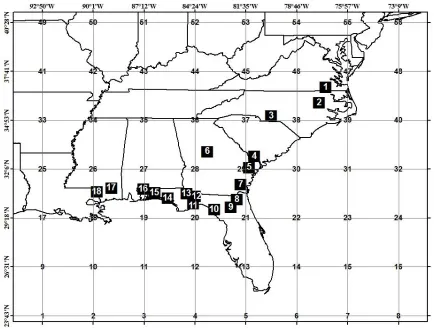
Figure 2.1 Location of the 18 HCDN stations along with the considered grid points
over the Southeast US ... 8 Figure 2.2 Simulated seasonal TN loadings for station, Nottoway river near Sebrell,
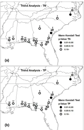
VA. ... 14 Figure 2.3 Trend Analysis, expressed as p-value from Kendall‟s Tau, of TN(a) and
TP(b) for 18 selected stations over the SEUS ... 15 Figure 2.4 Location of 18 water quality monitoring stations and grid points of
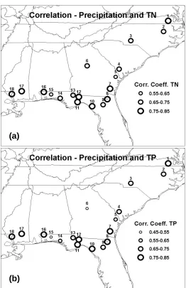
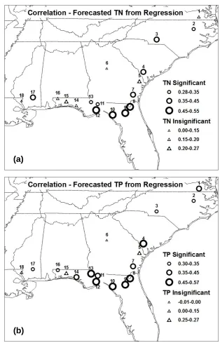
forecasted precipitation from NOAA‟s reforecast model ... 18 Figure 3.1 Rank correlation between the simulated nutrient (TN(a); TP (b)) loadings
and observed precipitation over the selected 18 stations ... 24 Figure 3.2 Correlation between the Loadest model estimates of winter TN and TP
loadings (using observed streamflow as predictor) and the regession model predicted loadings of TN and TP using forecasted streamflow obtained from the PCR model relating forecasted precipitation and observed
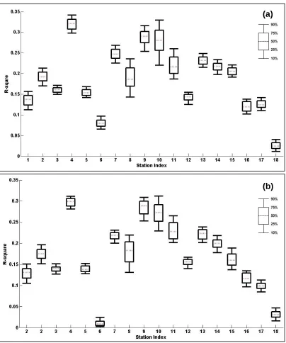
streamflow ... 32 Figure 3.3 Box-plot of R2 (based on equation (3.3)) of PCR model predicted TN(a)
and TP(b) loadings obtained using PC‟s of forecasted precipitation under LCV ... 34 Figure 3.4 Modified R2 (based on equation (3.3)) of PCR model predicted TN(a) and
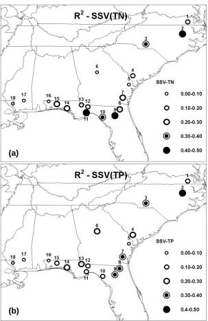
TP(b) loadings obtained using PC‟s of forecasted precipitation under SSV .. 35 Figure 3.5 Modified R2 (based on equation (3.3)) of PCR model predicted TN(a) and
TP(b) loadings obtained using PC‟s of forecasted precipitation under
MWV ... 36 Figure 3.6 Scree plot of the principal components on TN and TP loadings over 18
stations ... 40 Figure 3.7 Relationship between the first principal component of TN (a) and TP (b)
loadings over SEUS and ENSO conditions, which is indicated by Nino3.4 ... 41 Figure 4.1 Flow chart of the procedure to forecast TN and TP loadings ... 44 Figure 4.2 Box plot of rank correlation between observed daily streamflow in HCDN
and forecasted daily streamflow for each month from 1979 to 2009 ... 49 Figure 4.3 Rank correlation(a) and RMSE per unit area(b) between observed daily
streamflow from WQN and forecasted daily streamflow at the time of the TN observation in WQN ... 51 Figure 4.4 Rank correlation(a) and RMSE(b) between observed TN loading from
WQN and forecasted TN loadings for the observed values in the WQN
database ... 54 Figure 4.5 Rank correlation(a) and RMSE(b) between observed TP loading from
WQN and forecasted TP loadings for the observed values in the WQN
Figure 4.6 Correlation of TN(a) and TP(b) between observed concentrations from WQN and forecasted concentrations for the observed values in the WQN database ... 56 Figure 5.1 Tar-Pamlico River Basin, NC and 15 WWTPs participating water quality
trading program ... 60 Figure 5.2 Schematic procedure of utilizing forecast-based nutrient allocation in
water quality trading program ... 62 Figure 5.3 Flow chart for seasonal nutrient allocation conditioned on forecasted
seasonal loadings ... 66 Figure 5.4 Flow chart for daily allocation model development ... 68 Figure 5.5 Flow chart for an integrated nutrient allocation model development ... 70 Figure 5.6 Observed, Climatologic and Forecasted Seasonal TN loadings(kg/season) ... 72 Figure 5.7 Skill of daily loadings forecast model. Daily averaged observation and
forecast for winter season and correlation coefficient between observed
daily loadings and forecasted daily loading for winter season ... 73 Figure 5.8 Required seasonal TN loadings removal corresponding to LOADEST
(observation), Forecast, and Climatology ... 75 Figure 5.9 Excessive removal (
90 , 1 P i t i VL
) and Violated loadings (90 , 1 P i t i ER
) for winterseason in each year, which are ordered from dry year to wet year ... 78 Figure 5.10 The number of violated days over a winter season corresponding to the
different seasonal targets, 80% (a), 60% (b) and 40% (c) of climatology ... 81 Figure 5.11 Violated discharge (
90 , 1 i t i ER
) and Excessive removal (90 , 1 i t i VL
) for winterChapter 1
Introduction
Nutrient loadings and their concentrations at daily to seasonal time scales are primarily driven by streamflow which in turn depends on variations in weather and climatic conditions. This study focuses on relationship among climate, streamflow and nutrient variability over the Southeast US and on developing daily and seasonal nutrient forecast models contingent on weather and climate information. Using the developed daily and seasonal nutrient
forecasts, the study develops and evaluates a nutrient allocation model that controls point and nonpoint sources.
This dissertation is organized as follows: Chapter 1 presents the research objectives along with background and literature. Chapter 2 provides hydroclimatic and water quality databases employed in the study. Chapter 2 also develops daily nutrient loadings using the observed streamflow for 18 stations in the Southeast United States (SEUS). Chapter 3 evaluates the skill in developing nutrient forecasts in advance of a season using retrospective climate forecasts. Chapter 4 uses retrospective weather forecasts to develop daily
target seasonal loadings and desired nutrient concentration within the stream. Chapter 6 summarizes the findings along with the scope for future research.
1.1 Background and Research Objectives
Climate conditions are mainly driven by Sea Surface Temperature (SST) at seasonal and interannual time scale and similarly weather conditions are largely affected by initial
atmospheric conditions and land surface conditions. It is also well established in the hydroclimatic literature that variability in seasonal and daily streamflow can be partially explained using climate and weather infromation (Kingston et al. 2006; McCabe 1995). Considerable research now exists on the recurrence and regime structure of climate variables such as El Niño/La Niña-Southern Oscillation (ENSO) and Pacific Decadal Oscillation (PDO) and its teleconnections to rainfall/streamflow, and their potential predictability of interannual hydroclimatic variability over the United States (Ropelewski and Halpert 1987; Hamlet and Lettenmaier 1999; Dettinger and Diaz 2000; Devineni et al. 2008).
It is widely known that streamflow which can be predicted from climate and weather information is the most important predictor in estimating nutrient loadings and the associated concentration. For instance, streamflow variability predominantly influences instream
nutrient concentration due to loadings from both point and nonpoint sources (Borsuk et al. 2004; Paerl et al. 2006; Lin et al. 2007). Recent studies on relating coastal water quality conditions to Sea surface temperature (SST) conditions also show that there is a strong
aquatic vegetation (Cho and Poirrier 2005), and chlorophyll and phytoplankton levels (Arhonditsis et al. 2004). Joel et al. (2003) reported the effects of climate change on water quality in the Great Lakes Basin in the international joint commission report. However, systematic research in associating climate and weather information to seasonal and daily variability and utilizing that association to predict and control nutrient variability in watersheds is very limited. Thus, the main objectives of this study are to
(1) develop low dimensional predictive models to obtain pre-season estimates of
nutrient loadings over the Southeastern United States (SEUS),
(2) develop daily nutrient forecasts using retrospective weather forecasts, and
(3) develop seasonal, daily and integrated nutrient allocation models for improving
instream water quality.
1.2 Nutrient Allocation
The Clean Water Act (CWA) of 1972 was enacted with the objective of improving the physical, chemical and biological integrity of the Nation‟s waters (EPA 1972) and regulates pollutant discharges into streams from point sources by permit under National Pollution Discharge Elimination System (NPDES). US Environmental Protection Agency (EPA) implemented the Total Maximum Daily Load (TMDL) provisions of the CWA to accomplish water quality goals. TMDL estimates the maximum amount of a contaminant that a water body can receive and still meet water quality standards (Kibler and Kasturi 2007). EPA also emphasized that improvements on water quality under TMDL can be accomplished through market based approaches such as water quality trading rather than traditional command-control policy (EPA 2003). Water quality trading among point and nonpoint sources is intended for both developing control strategies and to reduce the cost of waste water treatment and nonpoint controls. One of the fundamental tasks in initiating a water quality trading market is setting up target loadings or caps on dischargers in order to achieve the desired water quality target (Horan and Shortle 2011). However, the absence of appropriate caps has resulted in lack of interest in establishing water quality trading (Hoag and Hughes-Popp 1997; King 2005; Ribaudo et al. 1999).
Various studies related to the allocation of point source loading have employed optimization models for waste load allocation (WLA) by employing stochastic, multi
2006; Sado et al. 2010; Cho et al. 2003). However, studies associated with loading allocation for nonpoint sources are rare owing to the uncertainties in estimating loadings from nonpoint sources. This uncertainty largely depends on unobserved loadings from individual nonpoint dischargers and uncertainty in nonpoint loadings due to unpredictable weather and complex environmental processes within the watershed (Shortle and Dunn 1986). Although a lot of variables need to be considered to define how much of loadings are coming from individual nonpoint sources, it is relatively simple to focus on predicting how much of total loadings are generated from a watershed under given climate and weather conditions. Therefore we try to utilize the forecasted seasonal and daily total loadings in the development of integrated, adaptive and multi-time scale nutrient allocation model.
1.3 Integrated, Adaptive and Multi-time scale Nutrient Allocation
For the development of an integrated, adaptive and multi-time scale nutrient allocation model, we firstly utilize seasonal nutrient loadings (developed in chapter 3) to set the target for nonpoint source reduction then nonpoint sources can develop appropriate best
management practices (BMPs) to comply with the target loadings. Once this is implemented, we can use the daily loadings (developed in chapter 4) for controlling point sources so that the desired concentration is maintained within the stream.
both point and nonpoint sources so that the desired seasonal target loadings and daily
concentration is maintained in the basin. For the seasonal nutrient allocation, we control only nonpoint source loadings and we assume the seasonal nutrient cap as a percentage of
climatological loadings but in practical, the cap can be defined by point-nonpoint
Chapter 2
Hydroclimatic and Water Quality
Databases
This Chapter summarizes climate, weather, streamflow and water quality databases employed in this dissertation. An estimation of daily nutrient loadings using observed streamflow is also discussed.
2.1 HCDN Streamflow Database
Given the intent of the study is to associate daily and seasonal nutrient loadings with weather and climate variability, we focus our analysis on 18 undeveloped basins over the Southeast United States (SEUS) from the Hydro-Climatic Data Network (HCDN) database (Slack et al. 1993). The HCDN database contains the mean daily discharge for about 1600 sites across the continental United States. The database includes streamflow records collected between 1874 and 1988, with an average station record length of approximately 48 years. Daily streamflow records in the HCDN basins is purported to be relatively free of
accuracy ratings of these records are at least „good‟ according to United States Geological Survey (USGS) standards. For the seasonal nutrient forecast model development, daily streamflow records are transformed to seasonal averages. Figure 2.1 shows the location of 18 HCDN stations and Table 2.1 provides the list of the 18 stations considered in this study along with their drainage areas. Since the streamflow data (Q) in the HCDN database is available only up to 1988, we have extended it up to 2009 based on the USGS historical daily streamflow database.
Table 2.1 Baseline information for 18 selected stations showing the number of years of observed daily records of nutrients available in the WQN database. Values in the parentheses under number of years column show the total number of daily
observations available for each station.
Station Index
Station
Number Station Name
Drainage Area (km2)
Number of Years (# of daily Obs.)
TN TP
1 2047000 Nottoway river near Sebrell, VA 3732.17 17(95) 18(96)
2 2083500 Tar river at Tarboro, NC. 5653.94 22(152) 22(156)
3 2126000 Rocky river near Norwood, NC 3553.46 14(65) 14(65)
4 2176500 Coosawhatchie river near Hampton, SC 525.77 13(100) 13(104)
5 2202500 Ogeechee river near Eden, GA 6863.47 20(141) 21(157)
6 2212600 Falling creek near Juliette, GA 187.00 14(56) 23(137)
7 2228000 Satilla river at Atkinson, GA 7226.07 20(123) 22(146)
8 2231000 St. Marys river near Macclenny, FL 1812.99 14(108) 14(113)
9 2321500 Santa Fe river at Worthington springs, FL 1489.24 21(82) 21(93)
10 2324000 Steinhatchee river near Cross city, FL 906.50 19(92) 20(96)
11 2327100 Sopchoppy river near Sopchoppy, FL 264.18 22(125) 25(170)
12 2329000 Ochlockonee river near Havana, FL 2952.59 22(133) 22(142)
13 2358000 Apalachicola river at Chattahoochee, FL 44547.79 23(152) 23(164)
14 2366500 Choctawhatchee river near Bruce, FL 11354.51 21(119) 21(128)
15 2368000 Yellow river at Milligan, FL 1616.15 21(123) 21(139)
16 2375500 Escambia river near Century, FL 9885.98 22(145) 22(151)
17 2479155 Cypress creek near Janice, MS 136.23 16(54) 23(100)
2.2 WQN Water Quality Observation Database
USGS provides national and regional descriptions of stream water quality conditions in Water Quality monitoring Network (WQN) across the nation (Alexander et al. 1998). The WQN database comprises water quality data from USGS monitoring networks from both large watersheds (National Stream Quality Accounting Network, NASQAN) and minimally developed watersheds (Hydrologic Benchmark Network, HBN). We employ the observed daily concentrations of Total Nitrogen (TN) and Total Phosphorus (TP) available for these 18 stations from the NASQAN. Observed streamflow during the time of sampling is also
2.3 Simulated Nutrients Database
Though nutrient data in WQN database is available for many years, their samplings are intermittent. To relate retrospective climate forecasts (discussed in the next section) that are available from 1957 onwards, we estimated the daily nutrient loadings from 1957-2009 using the observed streamflow data available from the extended HCDN database and the best fitting regression model, which is developed between observed nutrient loadings and observed streamflow on the day of sampling from the WQN database using the LOADing ESTimation (LOADEST) program developed by USGS (Runkel et al. 2004). Tables 2.2 and 2.3 show the “goodness of fit” statistics and the coefficients of the best-fitting regression model for TN and TP respectively for each of the 18 stations.
The LOADEST model allows the user to select the best-fitting regression model from eleven predefined regression models shown in Table 2.4 using the Akaike Information Criterion (AIC) (Akaike, 1974). Five regression models including „dtime‟ term are not appropriate to use for extrapolation since the term represents a linear trend in time that is present in the calibration data set. Therefore we select the best model over four regression models (i.e., model number 1, 2, 4 and 6). Utilizing this procedure, we ensure the simulated nutrient loadings from LOADEST program do not have any time trend. For details on the model forms, see Runkel et al. (2004). The estimated daily loadings from 1957-2009 are aggregated during January-February-March (JFM) to develop winter loadings (Lt) of TN and
available during 1957-2009 as the best information available for relating the interannual hydroclimatic variability to nutrient variability over 18 stations in the Southeast US (SEUS). We discuss in details about the uncertainty associated with using simulated values in section 3.2.3.
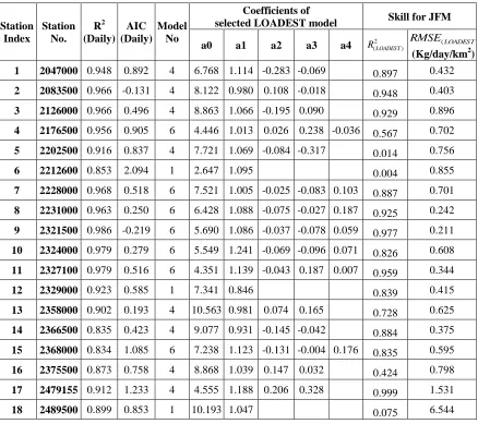
Table 2.2 Performance of LOADEST model in predicting the observed TN loadings from the WQN database. Models with linear time components (Model No: 3,5, 7-9) are not considered. The skill in predicting JFM WQN loadings (R(2LOADEST),RMSE(LOADEST)) are separately given in the last two columns.
Station Index Station No. R2 (Daily) AIC (Daily) Model No Coefficients of
selected LOADEST model Skill for JFM
a0 a1 a2 a3 a4 R(2LOADEST)
) (LOADEST
RMSE (Kg/day/km2)
1 2047000 0.948 0.892 4 6.768 1.114 -0.283 -0.069 0.897 0.432
2 2083500 0.966 -0.131 4 8.122 0.980 0.108 -0.018 0.948 0.403
3 2126000 0.966 0.496 4 8.863 1.066 -0.195 0.090 0.929 0.896
4 2176500 0.956 0.905 6 4.446 1.013 0.026 0.238 -0.036 0.567 0.702
5 2202500 0.916 0.837 4 7.721 1.069 -0.084 -0.317 0.014 0.756
6 2212600 0.853 2.094 1 2.647 1.095 0.004 0.855
7 2228000 0.968 0.518 6 7.521 1.005 -0.025 -0.083 0.103 0.887 0.701
8 2231000 0.963 0.250 6 6.428 1.088 -0.075 -0.027 0.187 0.925 0.242
9 2321500 0.986 -0.219 6 5.690 1.086 -0.037 -0.078 0.059 0.977 0.211
10 2324000 0.979 0.279 6 5.549 1.241 -0.069 -0.096 0.071 0.826 0.608
11 2327100 0.979 0.516 6 4.351 1.139 -0.043 0.187 0.007 0.959 0.344
12 2329000 0.923 0.585 1 7.341 0.846 0.839 0.415
13 2358000 0.902 0.193 4 10.563 0.981 0.074 0.165 0.728 0.625
14 2366500 0.835 0.423 4 9.077 0.931 -0.145 -0.042 0.884 0.375
15 2368000 0.834 1.085 6 7.238 1.123 -0.131 -0.004 0.176 0.835 0.595
16 2375500 0.873 0.758 4 8.868 1.039 0.147 0.032 0.424 0.798
17 2479155 0.912 1.233 4 4.555 1.188 0.206 0.328 0.999 1.531
Table 2.3 Performance of LOADEST model in predicting the observed TP loadings from the WQN database. Models with linear time components (Model No: 3,5, 7-9) are not considered. The skill in predicting JFM WQN loadings (R(2LOADEST),RMSE(LOADEST)) are separately given in the last two columns.
Station Index Station No. R2 (Daily) AIC (Daily) Model No Coefficients of
selected LOADEST model Skill for JFM
a0 a1 a2 a3 a4 R(2LOADEST)
) (LOADEST
RMSE
(Kg/day/km2)
1 2047000 0.934 1.255 4 4.129 1.219 -0.384 0.143 0.854 0.036
2 2083500 0.875 1.084 6 5.932 0.916 0.074 0.241 -0.062 0.946 0.046
3 2126000 0.912 1.388 6 5.844 0.896 0.064 -0.303 0.308 0.938 0.157
4 2176500 0.921 1.312 4 2.344 0.960 0.640 -0.290 0.795 0.025
5 2202500 0.862 1.1 4 5.253 0.943 -0.048 0.328 0.001 0.072
6 2212600 0.858 2.322 6 -0.228 1.305 0.075 0.387 0.058 0.900 0.238
7 2228000 0.841 1.262 4 5.075 0.619 0.092 0.116 0.565 0.141
8 2231000 0.854 0.983 2 3.404 0.760 0.062 0.943 0.011
9 2321500 0.877 1.165 6 4.291 0.708 0.039 -0.115 0.141 0.821 0.089
10 2324000 0.943 1.008 6 3.017 1.057 -0.058 -0.139 0.139 0.374 0.042
11 2327100 0.899 1.331 1 1.289 0.775 0.350 0.056
12 2329000 0.828 1.211 2 5.627 0.737 -0.036 0.785 0.060
13 2358000 0.857 0.912 1 7.778 1.321 0.815 0.039
14 2366500 0.812 1.036 1 6.267 1.213 0.779 0.036
15 2368000 0.799 1.554 4 4.374 1.320 -0.114 -0.133 0.568 0.053
16 2375500 0.864 1.134 4 6.182 1.220 0.106 -0.027 0.342 0.078
17 2479155 0.882 1.381 2 0.840 1.113 0.063 0.999 0.200
Table 2.4 Predefined regression models in the LOADEST model
Model
NO. Regression Model
1
2
3
4
5
6
7
8
9
10
11
* lnQ: ln(streamflow) – center of ln(streamflow)
** dtime: decimal time – center of decimal time, for each day of the year
Figure 2.3 Trend Analysis, expressed as p-value from Kendall‟s Tau, of TN(a) and TP(b) for 18 selected stations over the SEUS.
Figure 2.3 shows the p-value from Mann-Kendall test for winter TN (a) and TP (b) loadings estimated using LOADEST model. For the trend test, we employ aggregated seasonal loadings from daily loadings simulated using LOADEST program. At 1%
significance level, null-hypothesis with Kendall‟s tau being not equal to zero was rejected in
(a)
all of the sites for both TN and TP. Only two sites showed a significant trend at 5%
significance level for TN (four sites showed a significant trend for TP). We also performed regional Mann-Kendall test to account for spatial correlation among the 18 stations (Douglas et al., 2000). The p-values for TN and TP are 4% and 5% respectively indicating no spatial correlation. Thus, the trend analyses on individual stations and among stations on the extended (1957-2009) nutrient loadings show no statistically significant trend (at 1%
significance level) and provide the basis for explaining the interannual variability in nutrient loadings over 18 stations in the SEUS.
2.4 Climate Forecasts Database
In this study, we utilize the retrospective winter precipitation forecasts from ECHAM4.5, General circulation model, forced with constructed analogue SSTs (obtained from
http://iridl.ldeo.columbia.edu/SOURCES/.IRI/.FD/.ECHAM4p5/.Forecast/ca_sst/.ensemble2 4/.MONTHLY/.prec/, International Research Institute of Climate and Society (IRI) data library) (Li and Goddard 2005) to forecast winter seasonal nutrient loadings that can be provided at the beginning of the season. Retrospective precipitation forecasts from
Figure 2.1 also shows the locations of 56 grid points over SEUS of precipitation
forecasts from ECHAM 4.5 along with their latitude and longitude. For this study, we utilize only the forecasted mean (which is obtained by computing the average over 24 ensembles) of JFM retrospective precipitation forecasts issued in the beginning of January for developing the 3-month ahead retrospective nutrient forecasts over the period 1957-2007.
2.5 Weather Forecasts Database
We employed retrospective weather forecasts from National Oceanic and Atmospheric Administration (NOAA) to forecast daily streamflow which is in turn utilized to predict daily nutrient loading and the associated concentration. NOAA‟s Earth System Research
Laboratory/Physical Science Division (ESRL/PSD) reforecast project provides daily forecasted precipitation using the model from NOAA‟s Global Forecast System (GFS; formerly called the Medium-Range Forecast Model, MRF). Daily precipitation reforecasts is available from the GFS model consisting of 15 ensemble members in advance up to 15 days from 1979 to date. Since daily streamflow and nutrient variability is largely affected by daily precipitation forecasts, it is more appropriate to use daily streamflow forecasts for predicting daily nutrient loadings. Figure 2.4 shows 35 grid points over SEUS and the location of 18 stations. In this study, we employ daily reforecasted precipitation, issued on the day, to forecast daily streamflow for the period 1979 to 2009.
observed daily streamflow in HCDN database. Principal component analysis is applied on precipitation data on the identified grid points and these principal components are used as one predictor. For the other predictor, we employ previous three days averaged streamflow to account for soil moisture conditions. Then, nearest neighbor resampling method is employed to predict daily streamflow using above two predictors. The details will be discussed in Chapter 4.
Chapter 3
Seasonal Loadings Forecasts over the
Southeast US
measures utilized in developing and evaluating the season-ahead nutrient forecasts.
Following that, we present results from the dependency analyses relating winter precipitation forecasts from ECHAM4.5 GCMs with streamflow and nutrient loadings from the selected watersheds. Finally, in section 3.4, we present results from the winter nutrient forecasts developed using the principal components regression model utilizing the season-ahead precipitation forecasts and discuss the potential implications of the findings in the context of developing adaptive water quality management plans as well as in promoting water quality trading.
3.1 Introduction
The National Research Council (NRC 2002, NRC 2001) has emphasized that a detailed understanding of various sources of uncertainties, including the role of climate change and climate variability, is required for improving water quality prediction in natural systems. One of the dominant and well understood modes of global climatic variability is ENSO that has a periodicity of 3-7 years and exhibits anomalous warm/cold SST conditions in the equatorial Pacific, thereby modulating the climate particularly in the tropics and sub-tropics
2004, Paerl et al. 2006, Lin et al. 2007)and antecedent flow conditions (Vecchia 2003, Alexander and Smith 2006). Recent studies of the relationship between coastal water quality conditions and SST conditions also show that there is a strong association between climatic modes and concentrations of phosphorous (Childers et al. 2006), aquatic vegetation (Cho and Poirrier 200517), and chlorophyll and phytoplankton levels (Arhonditsis et al. 2004).
However, systematic research in associating climatic variability to instream nutrient variability and utilizing that linkage for improving water quality management is limited.
Most of the studies on estimating instream nutrient concentrations have focused primarily on predicting the average of annual concentrations using runoff and various basin attributes (Smith et al. 2003, Mueller and Spahr 2006, Mueller et al. 1997, Smith et al. 1998). Studies have also recommended approaches to predict daily and seasonal loadings and
concentrations of nutrients using streamflow and their time of observation (Cohn et al. 1992, Runkel et al. 2004). However, estimation of nutrient loadings/concentrations using
streamflow (Cohn et al. 1992, Runkel et al. 2004) primarily depend on the observed
information (e.g., streamflow) during that season, which has limited utility in developing pre-season estimates of nutrients. Findings from the hydroclimatic literature clearly show that interannual variability in streamflow can be predicted by developing low dimensional models contingent on SST conditions (Devineni et al. 2008) as well as using precipitation forecasts from General Circulation Models (GCMs) (Borsuk et al. 2004). Similarly, water quality literature emphasizes that streamflow is the most important descriptor in explaining nutrient variability (Cohn et al. 1992, Runkel et al. 2004). This study relates the interannual
develop low dimensional predictive models to obtain pre-season estimates of winter nutrient loadings over the SEUS.
3.2 Model Development and Performance Validation Metrics
3.2.1 Model DevelopmentGiven that winter streamflow over the SEUS is predominantly rainfall driven with limited snow accumulation, we hypothesize that precipitation is the primary driver in controlling the JFM loadings. To confirm this, we correlate simulated loadings using the LOADEST program with both observed precipitation and principal components of the forecasted precipitation from ECHAM4.5 (Figure 3.1). In this study, we only employ Spearman rank correlation for performing all correlation analyses and all the computed rank correlation was checked for statistical significance using equation (3.1) where „n‟ denotes the
number of data points used in calculating the correlation, „r‟ denotes Pearson‟s correlation
coefficient, and „z‟ implies the statistic follows normal distribution. Thus, the computed
correlation in Figure 3.1 needs to be greater than 0.24 (n = 51) to consider significant relationship between observed precipitation and simulated loadings.
3 ( ) 1.06
n
z F r (3.1)
where ( ) 1log1 tanh( )
2 1
r
F r arc r
r
.
Figure 3.1 Rank correlation between the simulated nutrient (TN(a); TP (b)) loadings and observed precipitation over the selected 18 stations.
(a)
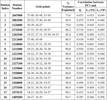
Table 3.1 Rank correlation between observed winter streamflow, TN and TP loadings with the first principal component of the winter precipitation forecasts for the 18 selected stations. Locations of grid points indicated in the Table are shown in Figure 2.1.
Station Index
Station
Number Grid points
% Variance Explained
Correlation between PC1 and
Q Lt (TN) Lt (TP)
1 2047000 37-40, 45-48, 53-56 73.6 0.453 0.453 0.449
2 2083500 29-32, 37-40, 45-48 84.9 0.479 0.476 0.486
3 2126000 36-39, 44-47 79.8 0.456 0.445 0.433
4 2176500 27-31, 35-39, 45-47 86.2 0.710 0.611 0.605
5 2202500 19-23, 27-31, 35-39, 45-47 85.6 0.598 0.480 0.473
6 2212600 37-40, 45-48 86.5 0.418 0.405 0.217
7 2228000 19-23, 27-31, 35-39 91.3 0.596 0.601 0.602
8 2231000 18-22, 26-30, 34-38 90.8 0.556 0.561 0.553
9 2321500 19-22, 27-30, 35-38 90.8 0.561 0.558 0.566
10 2324000 18-22, 26-30, 34-38 90.8 0.575 0.572 0.569
11 2327100 10-14, 18-22, 26-30 96.0 0.526 0.561 0.569
12 2329000 18-22, 26-30, 34-38 90.8 0.469 0.490 0.520
13 2358000 26-30, 34-38, 45-46 86.8 0.554 0.555 0.555
14 2366500 18-21, 26-29, 34-37 88.0 0.491 0.500 0.480
15 2368000 18-21, 26-29, 34-37 90.8 0.499 0.531 0.450
16 2375500 26-31, 34-39, 45-47 86.9 0.404 0.404 0.392
17 2479155 18-21, 26-29, 34-37 90.1 0.453 0.432 0.392
18 2489500 26-27, 34-35 94.7 0.287 0.284 0.296
3.2.2 Principal Components Regression
region are spatially correlated, employing precipitation forecasts from multiple grid points as predictors would result in multicollinearity issues in the development of the regression model. To avoid this, we employ PCR based on equation (3.2):
0 1
ˆ ˆ ˆ
( ) *
K
k
t j t t
k
ln L
PC
(3.2) where Ltdenotes the estimate of daily average nutrient (TN/TP) loadings during the JFMseason in year „t‟, PCtkdenotes the „k‟th PCs from the retained „K‟ PCs of precipitation
forecasts and ˆs denote the regression coefficients whose estimates are obtained by
minimizing the sum of squares of error. We employ stepwise regression to select „k‟ PCs out
of the identified grid points of precipitation (given in Table 3.1) for developing the PCR model. Stepwise regression is the step-by-step iterative development of a regression model that is related with automatic selection of independent variables. In this research, we develop a forecast model using only the first principal component and evaluate the model
3.2.3 Skill Scores for Nutrient Forecasts
To evaluate the skill in predicting the interannual variability in nutrient loadings using climate forecasts, we consider two error metrics – coefficient of determination (R2, defined in equation (3.3)) and root mean square error (RMSE, defined in equation (3.4)) per unit area of the watershed (A). However, these metrics need to be expressed considering the error in predicting the observed JFM nutrient loadings from the WQN database using the LOADEST program (R(2LOADEST),RMSE(LOADEST)) (see Tables 2.2 and 2.3) as well as the error in predicting simulated JFM nutrients from LODEST based on the PCR model (R(2PCR),RMSE(PCR))(see Tables 3.2 and 3.3). Since these two models are developed independently, R2and RMSE, in predicting JFM nutrient loadings using climate information could be expressed as follows:
2 ) ( 2
) (
2
* PCR
LOADEST R
R
R (3.3)
A RMSE
RMSE
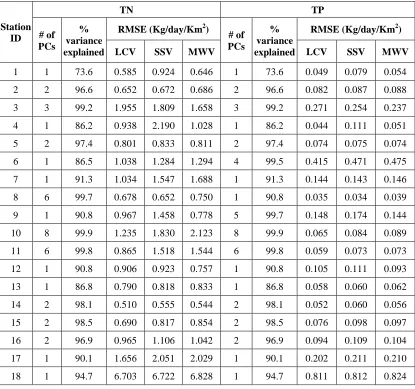
Table 3.2 Skill, expressed as RMSE (based on equation 3.4), in predicting winter TN and TP loadings using climate forecasts. Table also gives the number of principal
components considered and the percentage variance explained by them for the total grid points selected (given in Table 3.1) for each station.
Station ID
TN TP
# of PCs
% variance explained
RMSE (Kg/day/Km2)
# of PCs
% variance explained
RMSE (Kg/day/Km2)
LCV SSV MWV LCV SSV MWV
1 1 73.6 0.585 0.924 0.646 1 73.6 0.049 0.079 0.054
2 2 96.6 0.652 0.672 0.686 2 96.6 0.082 0.087 0.088
3 3 99.2 1.955 1.809 1.658 3 99.2 0.271 0.254 0.237
4 1 86.2 0.938 2.190 1.028 1 86.2 0.044 0.111 0.051
5 2 97.4 0.801 0.833 0.811 2 97.4 0.074 0.075 0.074
6 1 86.5 1.038 1.284 1.294 4 99.5 0.415 0.471 0.475
7 1 91.3 1.034 1.547 1.688 1 91.3 0.144 0.143 0.146
8 6 99.7 0.678 0.652 0.750 1 90.8 0.035 0.034 0.039
9 1 90.8 0.967 1.458 0.778 5 99.7 0.148 0.174 0.144
10 8 99.9 1.235 1.830 2.123 8 99.9 0.065 0.084 0.089
11 6 99.8 0.865 1.518 1.544 6 99.8 0.059 0.073 0.073
12 1 90.8 0.906 0.923 0.757 1 90.8 0.105 0.111 0.093
13 1 86.8 0.790 0.818 0.833 1 86.8 0.058 0.060 0.062
14 2 98.1 0.510 0.555 0.544 2 98.1 0.052 0.060 0.056
15 2 98.5 0.690 0.817 0.854 2 98.5 0.076 0.098 0.097
16 2 96.9 0.965 1.106 1.042 2 96.9 0.094 0.109 0.104
17 1 90.1 1.656 2.051 2.029 1 90.1 0.202 0.211 0.210
3.2.4 PCR Model Validation
To ensure that the skill in forecasting winter nutrients is reliable, we validate PCR models based on three different types of validation namely, leave-X out cross-validation (LCV), split-sample validation (SSV) and moving-window validation (MWV). Under LCV, the methodology suggested by Towler et al. (2009) is modified to evaluate the skill of the model over 51 years: (i) 10% of the data (5 years) are randomly removed along with the year for which the prediction is desired, (ii) a PCR model is developed using the remaining 45 years of loadings (Lt) and retained PCs (iii) the developed model is then used to predict the omitted year, and (iv) steps (i) and (ii) are repeated to develop prediction for each year and skill measures (R2and R-RMSE) were computed based on the 51 years of predicted data.
This entire procedure (i)-(iv) is repeated 100 times and a box-plot of R2 (Figure 3.3) and median of RMSE (in Table 3.2) are presented. Under split-sample validation (SSV), a PCR model is developed using Ltand PCs over the calibration period (1957-1986) and skill measures are computed based on the ability of the fitted PCR model in predicting Lt over the validation period (1987-2007). Another approach to validate the predictive models is to use a moving window of validation (MWV) considering the last „n‟ years (n=30 in this research) of
data, which forces the recent years of predictand and predictors being employed in
in Figures 3.3-3.5 and in Table 3.2 adjusted after accounting the error from the LOADEST model (equations (3.3) and (3.4)).
3.3 Results and Analyses
3.3.1 Nutrient Loadings Forecasts from Forecasted Streamflow
We investigate the ability to develop forecasts of winter loadings using
Table 3.3 Skill of the nutrient forecasting models developed using forecasted streamflow (as the predictor) which is obtained based on the PCR model developed between PF and observed streamflow. Third column in the table gives the coefficient of determination of the streamflow forecasting model (RQ2) under leave-one out cross-validation.
Station ID Station No.
R
Q2Forecasted streamflow
TN TP
R2 RMSE
(Kg/day/Km2) R
2 RMSE
(Kg/day/Km2)
1 2047000 0.382 0.153 0.401 0.154 0.033
2 2083500 0.420 0.173 0.523 0.173 0.069
3 2126000 0.399 0.151 1.712 0.141 0.217
4 2176500 0.570 0.324 0.595 0.320 0.035
5 2202500 0.543 0.245 0.226 0.238 0.015
6 2212600 0.317 0.091 0.571 0.012 0.343
7 2228000 0.550 0.310 0.607 0.312 0.022
8 2231000 0.497 0.253 0.506 0.241 0.029
9 2321500 0.565 0.318 0.658 0.322 0.105
10 2324000 0.538 0.291 0.811 0.301 0.039
11 2327100 0.488 0.275 0.683 0.283 0.020
12 2329000 0.417 0.193 0.715 0.221 0.078
13 2358000 0.511 0.260 0.466 0.259 0.041
14 2366500 0.438 0.265 0.389 0.245 0.040
15 2368000 0.396 0.266 0.433 0.210 0.056
16 2375500 0.357 0.126 0.533 0.120 0.052
17 2479155 0.387 0.135 0.611 0.109 0.033
Figure 3.2 Correlation between the Loadest model estimates of winter TN and TP loadings (using observed streamflow as predictor) and the regession model predicted
loadings of TN and TP using forecasted streamflow obtained from the PCR model relating forecasted precipitation and observed streamflow.
(a)
3.3.2 Nutrient Loadings Forecasts from the Developed PCR Models
Figure 3.3 shows the box-plot of R2 under LCV for 18 stations. Under LCV, we
compute R2 based on the predicted loadings for 46 years. Hence, R2 needs to be higher than 0.08 (correlation >0.29) to demonstrate statistically significant skill in predicting season-ahead nutrient loadings. From Figure 3.3, sixteen stations show statistically significant skill for both TN and TP. The developed PCR model under LCV explains more than 10% of interannual variability in both TN and TP nutrient loadings in all the 100 different fittings (Figure 3.3) except stations 6 and 18. For those 16 sites, the correlation between the predicted nutrient loadings obtained using climate forecasts and the loadings simulated from
Figure 3.3 Box-plot of R2 (based on equation (3.3)) of PCR model predicted TN (a) and TP (b) loadings obtained using PC‟s of forecasted precipitation under LCV
Figure 3.4 Modified R2 (based on equation (3.3)) of PCR model predicted TN (a) and TP (b) loadings obtained using PC‟s of forecasted precipitation under SSV
Figure 3.5 Modified R2 (based on equation (3.3)) of PCR model predicted TN (a) and TP (b) loadings obtained using PC‟s of forecasted precipitation under MWV
We compute R2 based on the predicted loadings during 1987-2007 using the model developed over the period 1957-1986 under the SSV method. Hence, R2 needs to be higher than 0.18 (correlation > 0.43) to demonstrate statistically significant skill in predicting
season-ahead nutrient loadings. Based on this, Figure 3.4 indicates that eleven stations (# 2-4, 7-11 and 13-15) show significant skill in predicting TN, and ten stations (#2-4, 6-9, 11, 13 and 14) show significant skill in predicting TP loadings. Insignificance in stations #6 and #8 could be explained by the reason of poor prediction by the LOADEST model because of the limited number of years of data availability, which is stated in the analysis under LCV method. From the Table 2.2 and 2.3, other stations (#1, 5, 12, 16 and 17) show either low R2 or high RMSE in the skill of LOADEST model for JFM. Thus, we infer that the skill of developed model under SSV is also affected by the ability of LOADEST model to estimate WQN nutrient loadings.
Figure 3.5a (3.5b) show the R2 in predicting the winter TN (TP) loadings under MWV and RMSE is included in Table 3.2. Though the performance under MWV is similar to the performance under SSV, we see a slight reduction in R-RMSE under MWV method. Overall, Figures 3.3-3.5 and Table 3.2 clearly show that the PCR model developed using the
3.4 Discussion
Analyses presented in this study (Figures 3.3-3.5) show that interannual variability in nutrient loadings could be predicted well before the beginning of the season contingent on the climate forecasts. By selecting grid points of precipitation forecasts that are statistically significant with the observed streamflow in the basin, we ensure that the skill in predicting nutrient loadings is related to the basin process as well.
Comparing Figure 3.2 with Figures 3.3-3.5, we infer that the skill in predicting the loadings remain similar even when using the forecasted streamflow. Thus, the skill in predicting the seasonal loadings exhibited in Figures 3.3-3.5 arises from the interannual variability in winter runoff resulting from climate variability. We understand the limitation in the developed nutrient forecasting models, which in fact employed simulated loadings (Lt) obtained using the observed streamflow based on the LOADEST models presented in Tables 2.2 and 2.3. Since obtaining long continuous records of daily observations of nutrients is difficult, particularly over a large region, we employed simulated nutrient loadings from the LOADEST model – which of course was fitted with observed daily loadings and streamflows from the WQN database – to understand the role of climate variability in modulating the interannual variability in nutrients over the SEUS.
Analyses presented here could also be extended to predict the season-ahead
analogous to the conditional distribution of seasonal streamflow – using the point forecast error related to equation (3.2). The conditional distribution of nutrients loadings could be effectively represented as an ensemble, which could in turn be utilized for estimating the probability of violating the desired loadings over the upcoming season. Analyses provided here also could be extended to other sophisticated statistical models in forecasting including nonparametric and Bayesian hierarchical models to develop conditional distribution of loadings.
monitoring those conditions could be beneficial for improving regional water quality and water quantity management. We have focused the seasonal forecasts on only winter season since two major reasons: (1) SST peaks during winter season and (2) hydrologic conditions are largely depending on local scale processes such as hurricane during summer season. Therefore, it needs more variables which are appropriate to account for local processes during the other seasons so that we also develop seasonal forecasts for other seasons.
Figure 3.6 Scree plot of the principal components on TN and TP loadings over 18 stations.
Seasonal nutrients forecasts developed in this chapter will be useful for controlling nonpoint sources in implementing the appropriate BMPs. This along with daily forecasts developed in Chapter 4 will be useful for developing a basin-wide nutrient allocation model.
0 10 20 30 40 50 60 70
1 2 3 4 5 6 7 8 9 10 11 12 13 14 15 16 17 18
Figure 3.7 Relationship between the first principal component of TN (a) and TP (b) loadings over SEUS and ENSO conditions, which is indicated by Nino3.4.
R² = 0.35
-6 -4 -2 0 2 4 6 8 10
-2.0 -1.5 -1.0 -0.5 0.0 0.5 1.0 1.5 2.0 2.5
PC 1 o f T N L o a d in g s (o v e r 1 8 Sta ti o n s ) JFM Nino3.4
R² = 0.34
-6 -4 -2 0 2 4 6 8 10 12
-2.0 -1.5 -1.0 -0.5 0.0 0.5 1.0 1.5 2.0 2.5
Chapter 4
Daily Forecasts of Nutrient Loadings
In this section, daily streamflow forecasts are developed for the prediction of daily nutrient loadings and concentration using forecasted precipitation (FP) from NOAA‟s
weather forecasts (Hamill et al. 2004) and the historical streamflow observation from HCDN database. We focus on the same 18 stations selected for development of seasonal forecasts in Chapter 3. The daily streamflow and loadings were developed using a semi-parametric resampling procedure (Souza Filho and Lall, 2003) that uses daily precipitation forecasts and previous month streamflow for finding neighbors from relevant previous years. The
forecasted daily streamflow and loadings are evaluated using observations from HCDN and WQN respectively.
4.1 Introduction
Continuous concerns about water quality degradation have forced active water quality management programs such as total maximum daily load (TMDL) allocation and
range. However, a river ecosystem is largely affected not only by loadings, but also by daily variations in streamflow. The US Environmental Protection Agency (EPA) suggests daily nutrient criteria for rivers and streams in ecoregions across the country (EPA 2007). To ensure that nutrient concentration complies with the suggested water quality standards, allowable amount of loadings from point sources could be determined if daily nonpoint nutrient loadings and streamflow is estimated in advance. Therefore, the main intent of this section is to develop a forecast model for daily streamflow and nonpoint nutrient loadings, which can be utilized to control point sources. Given this objective, we employ two predictors: forecasted precipitation from NOAA‟s weather forecast database (Hamill et al. 2004) (details were discussed in chapter 2.5) and averaged stremflow for the past 3 days before the forecasted date. The daily nutrients forecasting model development and validation are performed for 18 Hydro-Climatic Data Network (HCDN) watersheds over the Southeast United States (SEUS) which are described in detail in Chapter 2.
4.2 Methodology
The overall schematic diagram of the daily streamflow and nutrients forecasting methodology is shown in Figure 4.1. To perform this analysis, we first identify the grid points of NOAA‟s forecasted precipitation (FP) that correlate significantly with daily
relate the climate information to precipitation-runoff processes that control the streamflow from the watershed. Table 4.1 shows the identified grid points for each station (as indexed in Figure 2.3) of FP that are significantly correlated with daily streamflow, and the total number of significant grid points (in parentheses).
Figure 4.1 Flow chart of the procedure to forecast TN and TP loadings (NN: Nearest Neighbor method)
variables. Eigenvectors for each eigenvalue summarize the primary source (variable) of variability for that component (Devineni et al. 2008; Kaplan et al. 1998). In this analysis, we select the number of components that explains at least 90% observed variability of FP. Table 4.1 also shows the variance explained by the selected principal components (PCs), which typically ranges from 2 to 5.
Table 4.1 Selected grid points, the number of PCs selected for predictor, and Eigen Values of selected PCs (Grid numbers are shown in Figure 2.3)
Station
ID Selected Grids (total # of selected grids)
# of Selected PCs
Cumulative Eigen value of selected PCs
1 5, 7, 12, 19-21 (6) 4 0.962
2 5, 7, 12 (3) 2 0.905
3 4-5, 11-13, 18-20 (8) 4 0.948
4 11-13, 18-20, 27 (7) 3 0.909
5 17-18, 24-27 (6) 3 0.922
6 9-12, 16-19, 23-26 (12) 4 0.903
7 24-26, 31-33 (6) 3 0.918
8 17-19, 24-26, 31-33 (9) 4 0.918
9 17-19, 24-26, 31-33 (9) 4 0.918
10 16-19, 23-26, 30-33 (12) 5 0.921
11 16-18, 23-25, 30-32 (9) 4 0.930
12 16, 30-32 (4) 3 0.975
13 23-25, 30-32 (6) 3 0.934
14 18, 22-25, 30-32 (8) 4 0.938
15 18, 22, 24 (3) 2 0.912
16 22, 29-31 (4) 3 0.977
17 15-17, 22-24, 29-31 (9) 4 0.929
With the PCs of FP as a predictor for streamflow forecast, we employ 3 day-ahead average streamflow before the forecasted day as another predictor. For example, to forecast streamflow of Mar 14, predictors would be FP issued on Mar 13 (24 hours ahead) and average daily streamflow from Mar 11 to Mar 13. Thus, the number of variables varies from 3 to 6 (i.e., the number of selected PCs shown in Table 4.1 and 3-day average streamflow). Given these predictors, we utilize the k-nearest neighbor resampling method of Lall and Sharma (1996) with the neighbors identified by Mahalanobis distance (Mahalanobis 1936). Mahalanobis distance overcomes the two basic weaknesses in using Euclidean distance by employing a covariance matrix to compute the distance between points. (1) Variables with different units could also be employed and (2) the measure also accounts for the correlation among the variables. The Mahalanobis distance measure of a multivariate vector is defined by:
1
, ( ) ( )
T
i j i j i j
D X X S X X (4.1)
where Xi (X X1, 2, ,Xn),Xjare multivariate vectors containing predictor variables at
times i and j, T represents transpose operation, and S1 is the inverse of the predictor (X ) covariance matrix. In this analysis, „i‟and „ j‟represent forecasted the conditioning time step and the rest of the data available for calibration respectively (i j, 1, 2, ,31 and ji) with
2
n
.X
1 is 3 day averaged streamflow before the forecasted day, andX
2 is PCs of FPday, we consider 30 neighbors based on the Mahalanobis distance. Since the retrospective precipitation forecasts are only available from 1979, we consider additional neighbors by computing the Mahalanobis distance based on the 3-day average streamflow over the past four days. This results in a total 120 neighbors from which the forecasted streamflow for the given day could be developed. Then, we selected the nearest 50 neighbors over 120, and the 50 days streamflow provide the ensembles for predicting the daily streamflow. The
forecasted streamflow for each day is calculated as the conditional mean of 500 ensembles generated from the 50 neighbors whose density within the conditional distribution is weighted by kernel in equation (4.2) which is popularly used weight function in the field of hydrology.
1
1/ 1/
i K
j
i w
j
, i1, 2, ,K (4.2)where
K
50
(the number of neighbors),w
i represents the probability with which neighbor is resampled in constituting the 500 ensembles. LOADEST model is forced with theforecasted conditional mean to estimate the daily nutrient loadings at 18 stations. Since the model is calibrated with measured data from WQN database, the same model reported in Tables 2.2 and 2.3 are used to estimate the daily forecasted nutrient loadings. The
4.3 Results and Analysis
4.3.1 Streamflow ForecastsBattisti and Sarachik, 1995). Since weather phenomena in the summer season depend greatly on local scale processes, large-scale models do not have the ability to capture it. Hence, daily streamflows have high variability during summer season as well and are difficult to predict with high skill. From Figure 4.2, we also notice that the developed daily streamflow forecast model produces better results in winter and spring season than during the summer season.
Figure 4.2 Box plot of rank correlation between observed daily streamflow in HCDN and forecasted daily streamflow for each month from 1979 to 2009. Each plot includes 558 correlations (18 stations × 31years). Dotted line represents statistically
Figure 4.3 shows the rank correlation coefficients (4.3a) and root mean square error (RMSE) per unit area (4.3b) between observed daily streamflow and forecasted daily streamflow at the time of TN measurement from WQN database. Since concentration of TN and TP had been in large part recorded at the same time, we present here the streamflow forecasts skill only during the time of TN observations. Forecasted streamflows are
statistically significant at all stations, showing correlation coefficient greater than 0.8 in eight stations. Despite statistical significance in predicting streamflow for all stations, the model produces relatively high RMSE in stations, #11, 17 and 18 (Figure 4.3b). High errors in these stations are caused by failure to predict extreme flow values, which indicates the high
conditional bias in predicting extreme conditions. For instance, RMSE for station #17 drops from 3.56 to 0.54 by excluding only one extreme observation (recorded on 2/10/1981). The RMSE for the stations #11 and #18 is adjusted to 0.72 and 0.47, respectively, by eliminating one extremely high flow value in each station. Although this conditional bias is not observed in all stations, we infer that the daily streamflow forecast model has poor skill in predicting extreme flow values and this issue is discussed in detail in the section 4.4.
Figure 4.3 Rank correlation(a) and RMSE per unit area(b) between observed daily streamflow from WQN and forecasted daily streamflow at the time of the TN observation in WQN
(a)
4.3.2 Loadings and Concentration Forecasts
Using the forecasted daily streamflows developed in section 4.3.1, we estimate forecasted daily loadings using the LOADEST model on all the days for which WQN observations are available. Tables 2.2 and 2.3 provide the selected model number, the model performance, and coefficients for TN and TP, respectively. LOADEST model provides 11 different regression equations and the best model is chosen using Akaike information criterion (AIC). For this purpose, the conditional mean of the daily forecasts from section 4.3.1 is used as a predictor in the LOADEST model to estimate the forecasted daily loadings.
Figures 4.4 and 4.5 show the skill of forecasted daily loadings of TN and TP
Table 4.2 Observed extreme TN loadings and developed forecasts for them and
corresponding rank correlation and RMSE(kg/km2) with/without the extreme TN loading values. The rank is represented in the parenthesis next to the loadings.
Station Index
Given by the Model Extreme TN loading event
(kg/day)(rank) Without Extreme events
Correlation RMSE(kg/km2) Observation Forecasts Correlation RMSE(kg/km2)
3 0.79 4.04 90,423(1) 4,127(16) 0.79 1.20
43,018(2) 11,100(6)
17 0.54 6.66 6,729(1) 199(3) 0.51 1.30
18 0.69 3.54 342,820(1) 42,100(7) 0.61 1.02
319,828(2) 147,960(1)
Figure 4.4 Rank correlation (a) and RMSE (b) between observed TN loading from WQN and forecasted TN loadings for the observed values in the WQN database.
(a)
Figure 4.5 Rank correlation (a) and RMSE (b) between observed TP loading from WQN and forecasted TP loadings for the observed values in the WQN database.
(a)
Figure 4.6 Correlation of TN (a) and TP (b) between observed concentrations from WQN and forecasted concentrations for the observed values in the WQN database.
(a)
4.4 Discussion
The developed daily streamflow and nutrient forecast models represented in this study show that forecasted streamflow, TN and TP loadings have statistically significant
relationship in predicting the respective observation in the WQN database at all 18 stations over SEUS. By using forecasted precipitation and averaged streamflow for the past 3 days, we ensure that the performance in forecasting streamflow and loadings is related to the weather conditions and antecedent moisture conditions of a given watershed. The streamflow forecast model employs nearest neighbor method to generate forecast ensembles from
Mahalanobis distances between considered predictors. Using conditional averages of streamflow ensembles, the forecasted loadings are estimated from LOADEST model and associated concentrations are calculated as well. The forecasted daily streamflow, TN and TP loadings have statistically significant relationships with observed data in WQN in all 18 stations. For the forecasted TN concentrations, only two stations show insignificant relationship with the observation (one station shows insignificant relationship for the forecasted TP concentration). Despite these good skills in general, the developed model performed poorly when predicting extreme values in some stations. One possible reason for this poor skill in summer is due to the dominance of local-scale processes. Other possible reason is due to the methodology. Since we select neighbors out of historical measurements, the model does not produce forecast values beyond the maximum observation in the
probability that observation exceeds the forecasts. This could be a possible reason for the large differences in rank between observation and forecasts in Table 4.2. However, analyses provided in this research could be also extended to other sophisticated statistical models in forecasting, including Bayesian hierarchical models and probable maximum flow (PMF) estimation to develop probabilistic forecasts of daily flow and nutrient loadings.
In this analysis, the developed models show the ability to predict loadings and
Chapter 5
Multi-time Scale Nutrient Allocation
utilizing Climate and Weather forecasts
In this chapter, we develop a nutrient allocation model that utilizes nutrient loadings based on both climate and weather information to allocate nutrient loadings between point and nonpoint sources. For this purpose, pre-season nutrient loading forecasts developed in chapter 3 and forecasted daily nutrient loadings presented in chapter 4 will be utilized to develop an integrated multi time scale nutrient allocation model. We consider the daily and seasonal nutrient forecasts developed for the Tar River at Tarboro (station #2) (Figure 5.1). One primary reason for the selection of Tar River at Tarboro is because of its successful water quality trading program, which could benefit from the proposed nutrient allocation model.