An application of the transfer matrix approach for a dynamic analysis of complex spatial pipelines

Division III

AN APPLICATION OF THE TRANSFER MATRIX APPROACH FOR A

DYNAMIC ANALYSIS OF COMPLEX SPATIAL PIPELINES

Anatolii Batura1, Andrii Novikov2, Andrii Pashchenko3, Yaroslav Dubyk4

1

Ph.D, Lead Programmer, IPP-Centre Ltd, Kyiv, Ukraine 2

Ph.D, Head of the Department, IPP-Centre Ltd, Kyiv, Ukraine 3

Software Engineer, IPP-Centre Ltd, Kyiv, Ukraine 4

Mechanical engineer, IPP-Centre Ltd, Kyiv, Ukraine

ABSTRACT

An effective method for the calculations of stress and residual strength of complex spatial pipelines at static and dynamic loading with taking into account the vibration of internal liquid and Puasson coupling is presented. It based on the well-known transfer matrix approach. The method utilizes the exact mechanical equations for the stress-strained state of straight beam with distributed mass, which connect unknown parameters of forces and displacements at the end of beam calculation element with the parameters at the beginning of the element. At that general solution scheme and calculation models are the same for static and dynamic calculations, the only difference – are the equations. Two different methods are used to find natural vibration frequencies of the distributed mass system: straightforward (“brute force”) and quick, based on Williams-Wittrick frequencies counter. Within such counter a special procedure is developed for taking into account fluid vibration with consideration of volumetric balance condition at T-nozzles. The excellent accuracy of the method is demonstrated by the modeling of thin-walled, water filled pipe behavior after the rod impact.

Two seismic analysis procedures are implemented on the base of developed method: standard response spectrum procedure and normal-mode summation procedure (“exact” dynamical), which uses accelerograms.

These methods and procedures have been already implemented in calculation software complex for pipeline strength assessment with the possibility of building of arbitrary complexity models by the user-friendly, visual way. Their effectiveness is demonstrated by the seismic calculation for primary circuit pipings of Zaporizhia NPP.

INTRODUCTION

Complex spatial multibranched pipeline systems are widely used in the industry, in particular they are part of such critical objects as nuclear power plants, gas compressor stations of transit pipelines, petrochemical industry equipment, etc. The assessment of their stress-strained state at static and dynamic loading – is a key, basic task of their design and safe operation.

The most common method of dynamic analysis is the normal-mode method, which assumes that that pipe and internal fluid motion can be represented as a summation of natural vibration modes multiplied by functions of time. Obviously, the basis of such method is a solution of eigenvalues problem – finding of the natural vibrations frequencies and correspondent modes.

that a very large amount of degrees of freedom can be used and all practically valuable frequencies can be found. Moreover existing strength analysis softwares (e.g. ANSYS) have effective procedures of automatic building of such lumped-mass systems on the base of object model which minimizes possible errors and model preparation time.

However, such discrete mass approach has certain disadvantages concerning its application to elongated, multibranched pipeline systems. Quite complex procedure of model discretization is needed to build adequate model of piping, which can generally contain sections of absolutely different flexibility and length. The special “artificial” methods are needed to find force and moments components of the natural modes and to perform modeling of the kinematic excitation, etc. Also the application of mentioned lumped masses approach to such modern topical division of strength science as fluid-structure interaction is complicated.

It is well known that for an adequate analysis of such critical dynamical effects as water hummer or flow-induced vibrations it is necessary to consider the interaction that occurs between the pipe and the fluid (internal gas, liquid), see Wiggert and Tijsseling (2001). But exact theoretical solutions are known for the simplest systems only and mentioned discrete numerical approach can’t be applicable to real complex systems – in case of coupled vibrations enormous amount of calculation elements is needed for the fluid and pipe wall and great amount of additional fluid-structure interface elements is used to link metal and fluid elements, Moussou et al. (2000)! For this reason pipeline software packages (ASTRA, CAESAR) do not have the possibility of coupled fluid-pipe analysis, fluid is accounted as an added mass only!

The goal of this paper is to develop a relatively simple and effective method for harmonic vibration simulation of complex pipeline systems with taking into account dynamic behavior of internal liquid or gas. The restrictions of the existing lumped masses approaches should be taken into account.

The original variant of transfer matrix approach (TMA) for dynamic calculations with high accuracy and relatively simple implementation is presented. In accordance with it a piping is modeled as a system of beams with distributed masses, which is similar to above mentioned approaches for static pipeline assessment. Stress-strained state of the system is set by standard beam parameters in each cross section, which include 3-D vectors for displacement W , rotation angle , force Q and moment M , or totally 12 scalar parameters per cross-section. For taking into account a liquid vibration the list of beam parameters is extended: parameters of liquid displacement v and pressure P are added. In this paper harmonic processes are considered, i.e. proportional to sint, where  is some frequency of harmonic vibrations. Thus the cense of mentioned 14 parameters – is a vibration mode or deviation from the equilibrium position.

The well-known bottleneck of distributed-mass approaches is an extreme high difficulty of transcendental eigenvalues problem, which is a main barrier on their practical spread. To solve this problem a special extended variant of the frequencies counter of Williams and Wittrick is implemented with taking into account coupled liquid vibration.

The accuracy of the developed calculation methods is tested by a comparison with known theoretical results as well as with numerical calculation data. The practical significance of the methods is demonstrated on the example for seismic strength estimation for one of Ukrainian NPP.

THE DESCRIPTION OF TRANSFER MATRIX APPROACH FOR STATIC AND HARMONIC ANALYSIS

General Idea

for gas pressure distribution computation for the gas transportation network of arbitrary complexity and even for the solution of nonstationary thermal-mechanical task for pressure vessels at transient operational modes (Batura et al. (2014)), etc.

The approach is based on so-called transfer matrixes, which connect unknown parameters at the ends of calculation elements. In case of harmonic vibrations an expression for the element is following:

 



i



beginning end A l L

L  ,  (1)

Where A_i

 

,l is a transfer matrix for the ith calculation element having constant entries for considered frequency  and element length l, L - vector of 14 unknown parameters (12 beam and 2 liquid) for the beginning and end cross-sections of the element.

The common square matrix

 

A together with a vector of constant terms B for the whole pipeline system is filled by:

- transfer equations of type (1) for the all calculation elements;

- equilibrium and continuity equations for the connection nodes between neighbour elements; - boundary conditions.

Obtained system of algebraic equations is solved by a one of the many known methods and vectors on unknown parameters L are obtained for the ends of the elements. In the most cases (including considered problem of stress-strained state at static and harmonic loading) equations (1) can be easily written in a form which allows to obtain stress-strained state parameters in all internal points of the element on the base of obtained vector Lbeginning



.

Transfer equations for straight beams at static (Orynyak et al. (1998)) and harmonic (Orynyak et al. (2007)) loading are long known and easily obtained from the well-known differential equations for Euler or Timoshenko prismatic beams. For the demonstration purposes TMA equations for the axial and torsional vibration is presented below (here U and N – axial displacement and force,  and M_x - torsional angle and moment):

 

k x

k EF

N x k U x

U x

x met

x sin

cos 0

0 

 , N

 

x U₀EF_metk_xsink_xxN₀cosk_xx,

E

k_x2   ₍₂₎

 

k x

k GI

M x k

x tor

tor tor

x

x sin

cos 0

0 



 , Mx

 

x M0GItorktorsinktorxMx₀cosktorx,

G ktor



 2

(3)

Here the lover index 0 corresponds to the unknown parameters on the beginning of the element and x– is a distance from the beginning, to obtain Ai

 

,l transfer matrix substitution x=l should be used,

where l – is the element length. The standard notation is used for the pipe/beam properties: E and G–

Young and shear modulus, Fmet – the cross-section area of the metal part of the pipe, - the metal density, I– torsional cross-sectional inertia moments.

Extension for Taking into Account Poisson Fluid-Metal Coupling

In this pipe two the most important mechanisms of fluid-pipe coupling: junction and Poisson coupling are considered. Such mechanisms as friction and Burdon coupling are assumed to be insignificant for the real industrial pipelines.

Poisson coupling is conditioned by interconnection between axial pipe deformation and radial deformation of pipe cross-section, caused by Poisson effect. Differential equations for taking into account a mutual influence of axial pipe vibration and internal fluid vibration were proposed by Skalak:

 

 

 

E F

t x N hE

RK K

t x P x

t x v

met f

f

, 2 2

1 ,

, _{ }

   

 

 

 

 

 

2 2 , , t t x v x t x P f     

  (4b)

 

 

 

hE R t x P E F t x N x t x U met , , , _{ }    _(4c)

 

 

2 2 _, , t t x U F x t x N met     

  (4d)

Here v ‒ fluid longitudinal displacement, P ‒ the fluid pressure pulsation, h ‒ the pipe wall thickness, R‒ the inner radius, _f – the density of the fluid,  – Poisson’s ratio, K_f – bulk elasticity of fluid.

After transformations and reduction of sint two joint equations are obtained, here we used modified bulk modulus

1 2 1          hE RK K

K _f f :

E U K v dx v

d _2 f _2  2 2 2    (5a) hE R v E F U dx U d f met    

2 2

2 2

 

 (5b)

The solution of (7) and (8) presented in details in Dubyk and Orynyak (2016). The transfer matrix

 

l

Ai , for the 4 joint parameters U, N, v and P is presented below, it’s split into 4 parts for the better presentation (here F– the cross-sectional aria of the fluid (FR2)):

 

                          0 0 0 0 1 1 1 1 P N v U A P N v U

i ,

 



      4 3 2 1 A A A A

Ai (6)

 

              ) ( cos ) ( 2 ) ( 2 1 ) ( cos 2 2 2 2 2 1 4 x F x RF h x F F h R x F x F x A y x       (7d)

Following notations have been used:

E

a2  ,  1 2 _2

       hE RK K d f f f

,

   

₂

2 2 1 2      a

x , F₁(x)sin₁x ₁sin₂x ₂, 1

) 2 1 /( 1

1  

   , hE RKf  1

 ,

   

2

2 2 1        d

y , F2(x)cos1xcos2x,

 

2 8 ) ( )

( 2 2

2 2 , 1  

  ad  ad  ad ,

   

 

   

 

2

2 2 1 2 2 2 2 2 1 2 1             

 a d , F3(x)1sin1x2sin2x.

Thus obtained equations (10) are an extension of (3) with additional taking into account of fluid vibration. Despite they form is relatively complex, they don’t degenerate for any fluid and pipe parameters and any Poisson’s ratio µ and can be easily implemented within TMA.

Boundary and Continuity Conditions

Standard mechanical equations for the connection nodes are very easy: 1) continuity conditions:

n

W W

W₁ ₂ ... ,   n

  

... 2

1  (8a)

2) equilibrium conditions:





 j

out j i

in

i Q

Q  ,







j out j i in i M

M  (8b)

Here unknown variables in global spatial coordinate system notation are written for the ends of the elements, which are connected in the node, lower index – is a number of the element, in denotes incoming elements (connected to the node by their conditional ends) and out – outgoing elements (connected by the beginnings). Equations (8) are proper for a case of angular connections between the elements. And this allows to model pipe bends, which are presented as a set of straight pipes, connected in consequence with certain small angle between neighbor elements. Generally, static theoretical solution in a closed form for the bend is long known, but obtaining of dynamical solution is extremely complex task associated with a solution of 6th order equation and can be solved for some particular cases only. Thus modeling of pipe bend by the straight pipes is preferable for the practical implementation, especially since it provides high accuracy and calculation speed, Orynyak et al. (2007).

The equilibrium condition for the fluid pressure is very simple:

n

P P

P1 2 ... (9)

Continuity condition considers fluid volume continuity with taking into account axial vibration displacement U of the pipe, written in the local coordinates for each element:













  j j j j

i

i i

i v U F v U

F

out in

Equation (8b) for the forces equilibrium should be extended to take into account pressure pulsation, where unit vector t directed along the pipe axis (corresponds to local pipe displacement U and fluid displacement v):



 







  j j j j j

i

i i i

iPt Q F Pt Q

F

out in

  



(11)

Such notations are also applicable for a case of angular elements connections, including the modeling of a pipe bend.

For support taking into account within TMA additional variables per each support direction (constrained pipeline degree of freedom in support cross-section) are introduced. Let’s consider support reaction – an unknown variable r, dealing along direction g (unit vector). Condition (8b) should be extended:





 j  

out j i

in

i Q r g

Q   (12)

Additional equation for movements is following:

 

W;g crV (13)

Here c – a compliance of the support and V – an initial movement. In case of absolutely rigid support s=0 and displacement W is specified by V. And for non-zero V value in case of dynamic task the kinematic excitation is obtained. Also usage of (12) with certain known constant value r allows to simulate concentrated force, (13) is not needed in that case. Equations for the moment supports/forces are similar.

The boundary conditions for a beam are obvious and can be easily get from (8), (12), (13) expressions. At that fluid has two types of boundary conditions:

0 

P (14a)

U

v (14b)

Equation (14a) set boundary condition of type “barrel of infinite volume” and (17b) – closed pipe end. Universal form of (14) can be written as follows:





1

1

1  

 P vU  (15)

The coefficients ₁,₁,₁ set the ratio between (14a) and (14b). It should be taken into account, that for the simplest cases the choice of (14)-(15) expressions is obvious, but for the most of the real cases of practical interest, such as mechanically isolated with a containment wall part of NPP steam pipeline, the choice is complex and ambiguous. Energetic approach for acoustic boundary conditions choice is described in Orynyak et al. (2015).

A DETERMINATION OF NATURAL FREQUENCIES AND MODES. WILLIAMS AND WITTRICK APPROACH

General Idea of a Frequencies Counter

TMA deals with distributed mass beam systems. The correspondent beam equations contain transcendental functions and there is no stable universal solution method for correspondent eigenvalue problem. The possible brutforce, straightforward natural frequencies determination algorithms have huge calculation time and essential danger of frequency miss even for a relatively simple beam system.

In 1970th by Williams and Wittrick a special counter (WWC) was proposed which gives a number of natural frequencies, which not exceed certain test value ₀, see Williams and Wittrick (1970). This counter is relatively simple in implementation, has quite high calculation speed. Therefore it can be obviously used to effectively find all necessary natural vibration frequencies of complex multibranched beam system with a prescribed accuracy, e.g. by the bisection method. WWC is described in large numbers of papers, Banerjee and Williams (1994), and can be also generalised for a problem of beam stability (Williams and Wittrick (1983)), etc.

WWC is based on dynamic stiffness approach (DSA). General DSA equation for a distributed mass system is following:

 



K 



W F (16)

Here K – is a dynamic stiffness matrix, W - displacements of each degree of freedom of all model nodes in global coordinates, F - vector of external excitation forces, applied to each node. Considering natural (free) vibrations, condition F0 should be provided, which is possible at W 0 and at condition (17):

 

 0

K (17)

These two conditions allow to formulate the idea of WWC. Imagine that certain test frequency 0

 is fixed and all elements of K

 

0 matrix are calculated and presented as real numbers. To get value of K

 

₀ Gauss elimination process should be applied (the only allowed operation – the subtraction of the previous row, multiplied on a certain coefficient, from the current row) and upper triangle matrix

 

0



K should be got. The product of diagonal elements of K

 

₀ is equal to K

 

₀ . At that total amount of the natural frequencies below ₀ is equal to a sum of two counters:

- Counter 1, the amount of the negative elements on the diagonal of K

 

₀ ;

- Counter 2 – is a sum of the amounts of theoretical natural frequencies for all calculation elements in the model, which are supposed to be the separate and be rigidly clamped at the both ends each. Such number can be trivially obtained on the base of well-known theoretical solution for a straight beam.

The idea of WWC comes from the process of Gauss elimination during the calculation of

 

0

K . The first diagonal element of K

 

0 is taken unchanged to the total product. The second element is transformed into the fraction, where the first diagonal element – is the denominator. The obtained second element is the denominator of a transformed third element, …. and the last element N (actually, it determines the roots of the whole system) after transformation got element N-1 as denominator. So, we got a chain, where at intermediate roots a pair of the diagonal elements mutually changes their signs to the opposite (the number of “minuses” stays unchanged) and the total amount of negative diagonal elements changes at the root of the whole system only, when element N changes the sign. The strong prove of WWC adequacy is presented in Williams and Wittrick (1970).

A Procedure for DSA Matrix Construction

The key question of WWC is a process of DSA matrix construction. Within DSA ideology, displacement variables Wi



for a connection node are common for all connected elements ends. Matrix K

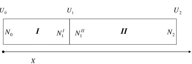
is filled on the base of (8b) force balance equations, where force summands are obtained on the base of displacements of connected elements. Let’s illustrate it on the base of simple example of axial vibration of two connected beams (Williams et al. (2002)), see fig. 1.

Boundary/balance equations for nodes 0,1,2 are following: 0

0 

N

;

N₁II(N₁I)0

;

(N2)0

.

(18)

І

N

₂

1

U

0

U

X

0

N

ІІ

2

U

I

N

₁

N

₁II

Figure. 1. The vibration of two straight beams system

After transformations on the base of known equations for axial beam vibrations, K is obtained:

















































II

k

II

k

II

k

II

k

I

k

I

k

I

k

I

k

K

II II

II II

I I

I I

cot

cosec

0

cosec

cot

cot

cosec

0

cosec

cot

(19)

Here simplified notation is used, where kIcotI kImetEIFImetcot



kImetlI



, I

I met

I E

k   , lI – element I length and the same – for element II. In (19) components of separate matrixes for element I and II are highlighted. It can be seen that for mechanical vibrations matrix K is formed by simple joining of the matrixes for each calculation element, thus it makes process of K building quite simple.

The important sign rule should be always fulfilled. Theoretically the signs for each row of K can be chosen in arbitrary way, it doesn’t influence on the correctness of balance conditions. But sign change violates sings on K

 

₀ diagonal and value of WWC. The starting point for WWC correct work is such a sign choice of K rows that for 0 diagonal elements of K should be positive, in other case rows with negative diagonal element should be multiplied by “-1”. The diagonal elements correspond to such global displacement direction, which is codirectional with global force whose balance is described by a correspondent row of K. This rule is very important for further fluid taking into account.

 

      

i i i i global global i global global G B G K W W K Q Q 1 2 1 2 1 ,                         (20)

Here Q– are the forces/moments vectors, W– displacements/rotations vectors, 1 – index of the conditional element beginning, 2 – index of the element end, Bi – DSA matrix for the element i in the local coordinate system, Gi– rotation matrix which transform global model coordinates into the local for the element. Sign “-” at Q2global



is needed to provide fulfilment of (8b) conditions and sign rule.

TMA and DSA are based on the same known equations for a beam. Despite Bi matrixes for a straight beam are long known, on the base of block-wise matrix inversion the expression (21) was obtained which allows to get Bi from the TMA matrix of the element:

 





                                      1 1 1 1 1 1 2 2 , B D A B D C B A B i local local D C B A local local M M M M M M M M M B Q W M M M M Q W     (21)

Here MA – square submatrix, which corresponds to components of W1local



in the expressions for

local

W₂ and so on. Expression (21) is universal and can be used for Euler or Timoshenko beam equations as well as for equations of type (6)-(7).

Principles of the Fluid Taking into Account

The feature of DSA matrix is that amount of unknown variables as well as amount of the equations is the same for each node, and this is a difference in comparison with TMA. This principle should be saved for the coupled metal/fluid vibrations. For this type of modelling one variable of fluid displacement v and one equation of the pressure P balance should be added.

For the closed end metal boundary condition should be extended according to (11) and additional condition (14b) for a fluid should be used. If boundary element have stiffness submatrix K/ (22) which corresponds to coupled axial metal and fluid vibration (obtained on the base of (7) transformation according to (21) expression), the first row of submatrix (23) is a DSA analogue of (11) for a free closed end 1 and the second row – the analogue of (14b):

 

 

                                            44 43 42 41 34 33 32 31 24 23 22 21 14 13 12 11 2 2 1 1 2 2 1 1 ,                 K v U v U K P N P N (22)





             0 0 1 1 24 14 23 13 22 12 21

11       

 F F F F

Kliquid metallfreeclosedend (23)

It can be seen that second row of (23) fulfills the sings rule. Here and below in this chapter equations are given for a collateral elements for the simplification, (20) should be used in general case to take into account angle between the elements.

Taking into account open free end condition (14a) is trivial – two first rows of (22) should be used.

The difficulty of fluid vibration taking into account within DSA is gap of fluid displacement v in nozzles or places of pipe cross-section area change according to (10). This is no problem for TMA, because separate variables for each element end are introduced in the connection node, but special approach should be developed for DSA.

І

N2, 2 P 1 U 0 U 0

N

ІІ

2 U

I N₁,

I P1

II

N

₁ ,

II P₁

ІІ

I

III N1 ,

III P₁ 3 N , 3 P II v1 I v1 III v₁ 0

v v₂

3 v

Figure. 2. The vibration of three fluid-filled straight pipes

The conditions of two equations should be fulfilled in DSA matrix: III

II I

P P

P₁  ₁  ₁ (24)



 

 

III



I III II I II I I I P F N P F N P F

N₁  ₁  ₁  ₁  ₁  ₁ or, with taking into account (24),



 

 

I



I III I I II I I I P F N P F N P F

N₁  ₁  ₁  ₁  ₁  ₁ (25)

For the sake of certainty let’s consider that additional variable of fluid displacement is v₁I

(element I) and the only equation for P is P₁I P₁II. Therefore equation P₁I P₁III and variables v₁II, v₁III

should be taken into account implicitly. From the expression of type (22) for element I equations for P₁I

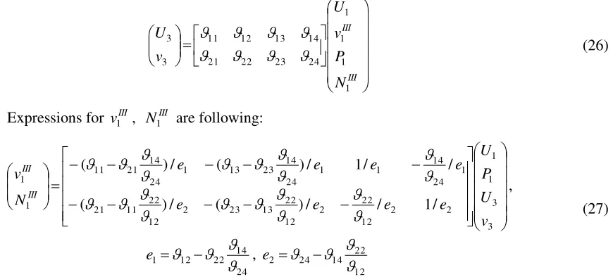
and N₁I are obtained a-priory. Thus unknown variable P₁III can be changed by equation for P₁I on the base of (24). Let’s consider TMA expression of type (7) for element III:

                           III III N P v U v U 1 1 1 1 24 23 22 21 14 13 12 11 3 3         (26)

Expressions for v₁III, N₁III are following:

                                             3 3 1 1 2 2 12 22 2 12 22 13 23 2 12 22 11 21 1 24 14 1 1 24 14 23 13 1 24 14 21 11 1 1 / 1 / / ) ( / ) ( / / 1 / ) ( / ) ( v U P U e e e e e e e e N v III III                     , 24 14 22 12 1 _      e , 12 22 14 24 2 _      e (27)

If several pipes connected in a node, expression (27) can be applied for the element IV, V and so on. Having the expression for v₁III, expression for v₁II is following (got on the base of (10)):









II III III I I II F U v F U v F

v 1 1 1 3

1

 



And having displacement parameters at the ends of the element II, expressions for N₁II and P₁II

are obtained easily by the definition of stiffness matrix and equations (25) and P₁I P₁II can be filled. It can be easily seen, that such principle is correct for the two pipes junction, at that v₁III 0 and (27) is not used.

Thus for taking into account fluid vibration, one additional variable is introduced in each connection node and one pressure balance equation is added for a node. For a case of multiply connection additional fluid variables and equations for a pressure balance are taking into account implicitly. The general principle for fluid taking into account in DSA and WWC is formulated.

A Procedure for Natural Mode Obtaining

Presented modification of Williams and Wittrick frequencies counter has moderate implementation complexity and high calculation speed. Its bottleneck is obtaining of the natural vibration modes, which correspond to obtained frequencies within the ideology of DSA. Even for the lumped mass case such a task demands complex iteration process for each found natural frequency, and for the distributed mass systems this process is still more complex and contains matrix linearization, differentiation and inversion, as well as additional system splitting into calculation elements (Yuan et al. (2003)), these operations on huge matrixes of real pipeline systems take a lot of computer time. And natural mode values for the internal forces and moments are often obtained by additional complex process, usually on the base of static calculations, when beam system is loaded by certain distributed force, proportional to natural mode displacement. This method is widely used in known standards, such as Soviet Union nuclear standard PNAE G-7-002-86 (1987).

Implemented TMA allows to easily obtain natural vibrations modes on the base of found array

 

i of natural frequencies by so-called displacement disjunction method. In arbitrary connection node between two elements one of the conditions (8a) for a chosen global direction (e.g. along global X axis) is excluded. Instead it a certain non-zero displacement along that direction is set for one of elements end:

0 1 

X

W (29)

The continuity condition is broken here, but if such displacement corresponds to real natural vibration mode, there is no displacement gap in this point after the solution of the matrix for a natural frequency i:

   



 X X X X

W W

W

W _{1 2} , (30)

The situation when (30) is not fulfilled is possible if the correspondent node is a vibration node at frequency i and theoretical solution is 1  2 0

X X

W

W . Thus the other disjunction node or global direction should be chosen for TMA application. After the matrix solution in one iteration all displacement and force parameters are obtained for all elements ends, which forms natural vibration mode. Modes for a multiply frequencies can be easily separated by the modes orthogonality law.

You can pay attention that dependencies of values (30) and (17) on a frequency  can be used for a brutforce, straightforward natural frequencies determination algorithm for TMA and DSA correspondently. However, these methods for distributed mass systems can be used for test purposes only.

TEST CASES. A SIMULATION OF STRAIGHT PIPE DYNAMIC BEHAVIOUR AFTER A STEEL ROD IMPACT

modes were obtained for an in-plane vibration of 3-pipes junction (T-nozzle) by TMA (by a brut-force root search method) and WWC.

Length of the first pipe l_I=5 m; l_II=4 m; l_III =3 m; Young modulus E for all pipes 2*1011 Pa; shear modulus G=8*1010 Pa; wall thickness h1=2.5mm; h2h3= 3.5mm; outer radius r1=30mm;

3 2 r

r  =40mm. Two densities were considered:



 7800 kg/m3 and 3000 kg/m3.

The results (first natural frequencies) are shown in the table 1. There the Counters are changed exactly on the natural frequencies. Note that for 0 there are 3 frequencies exist. They correspond to the undeformated movement of such unanchored pipeline system in 2 directions and rotation in 1 direction. Two first natural vibrations modes are shown on fig. 3 (no 2 and 3 from table 1), they are obtained by the TMA displacement disjunction method.

Table 1. Natural vibration frequencies for in-plane vibration of T-nozzle, Hz

N of

frequency  7800 kg/m

3 _

3000 kg/m3 Counter 1 + Counter 2

1 0 0 3

2 3.016 4.864 4

3 8.602 13.871 5

4 14.410 23.234 6

5 26.619 42.923 7

6 39.862 64.277 8

Figure 3. Natural vibration modes #2 and #3 for T-nozzle

The liquid vibration in T-nozzle was modelled to test the correctness of DSA matrix construction. Parameters are as follows: lI=4.51 m; lII =lIII =1.34 m; Young modulus E for all pipes 168 GPa; wall thickness h=3.945mm; inner radius R=26.01 mm. Liquid density f  999 kg/m

3

, bulk modulus

K=2.14 GPa. Comparison with analytical solution demonstrates that proposed method for fluid T-nozzle modeling within DSA ideology is correct, see table 2.

Table 2. Natural vibration frequencies for a liquid vibration in T-nozzle, Hz.

Test

freq. 0 103.25 228.78 252.66 357.86 470.33 567.79 686.77

WWC

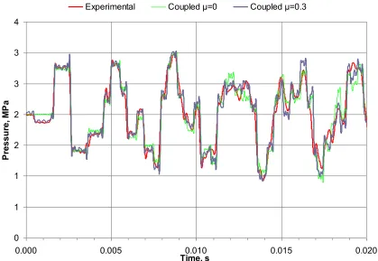
To demonstrate power of the developed approaches for the internal fluid vibration simulation, the behavior of a fluid-filled pipe, closed at both ends and subjected to axial excitation was modelled (Zhang et al. (1999)). The pipe is suspended on wires and is excited be axial impact of a 5 m long, 51 mm diameter steel rod.

The pipe parameters, different from previous example: l_I=4.502 m, 7985kg/m3, 0.3. On the left there is cap about 60 mm thick, on the right cap about 5 mm. Natural frequencies results are presented in table 3. They are obtained by both WWC and TMA brutforce metod and compared with experimental data.

Table 3. Natural frequencies (in Hz) of axial vibration of water-filled pipe with free ends.

N of frequency

Mechanical Acoustical Coupled Experimental (Zhang et al.,

1999) ρ=7985 ρ*=11046 с=1464 с*=1354 μ=0 μ=0.3

1 509 433 163 150 169 172 173

2 1019 866 325 301 288 286 289

3 1528 1299 488 451 453 453 459

4 2038 1733 650 602 493 493 485

5 2547 2166 813 752 629 633 636

6 3057 2599 975 902 743 741 750

7 3566 3032 1138 1053 906 907 918

8 4075 3465 1300 1203 980 980 968

Here   f f

K

c _ speed of sound in fluid, or with the wall expansion correction

f

K c _ ; ρ* - is a density of pipe metal with added mass of the fluid. Theoretical frequencies for uncoupled separate vibration of metal and liquid are trivial and obtained calculation results match them. Coupled frequencies (with only junction coupling at the ends and with Poisson coupling) are close to experimental. However, in this example as well as in most of real NPP pipelines, influence of Poisson coupling on natural frequencies is quite small, in contrast to its influence on natural modes, which is noticeable in general. Also Poisson coupling is important for relatively thin-walled pipelines, such as oil transit pipelines.

The idea of normal-mode method is described by the following expressions:

 





   



 

1 ,

i

i x t

t x

v  (31a)

 





   



 1 ,

i

i x t

X t

x

U  (31b)

Here _i and X_i are eigenfunction (normal modes) for eigenvalue _i, for mechanical and fluid displacement. The axial displacement is considered for a distinctness

The response of the ith vibrational mode is found by the Duhamel integral to be:

 

 









 

















 



 

 



l

i i

met i

i l

i i

f i i i

dx d t m

Q x X

dx d t m

Q x t

0 0

1 2

0 0

1 2

sin ) 2 1 ( 1

sin ) 2 1 ( 1

 

     

     



Here





i l

f i p

im m dx m

X  



0

2

2~ ~ _,





1 2 2 1

~ _{ F   }

mp f ,



1



2 2 1 ~ _{  }

met f F

m . Qf and Qmet - outer excitation forces, applied to fluid and metal. To simulate this experiment, we have suddenly applied force Q_met0 15.4 kN at one end (z=0) for a duration of  2ms, causing axial waves to propagate along the pipe. For simplicity force is schematized in such form, the real force form should be computed from dynamic problem solved both for rod and for pipe. Integration result for (32) is as follows, where X_i0 - is a metal displacement at point of rod impact for ith normal mode:

 



 











 





     

 

 

 





 

  

 

 

   

t t t

m Q X

t t m

Q X t

i i

i i met i

i i

i met i

i

; cos cos

) 2 1 (

; cos 1 ) 2 1 (

2 1 2 0

0

2 1 2 0

0

(33)

Pressure distribution at the pipe center is presented on fig.4. for junction coupling and Poisson and junction coupling. Influence of Poisson coupling is about 10% for a such thick pipe.

0 1 1 2 2 3 3 4

0.000 0.005 0.010 0.015 0.020

Time, s

P

re

s

s

u

re

,

M

P

a

Experimental Coupled µ=0 Coupled µ=0.3

Figure 4. Measured and calculated pressures at pipe middle (x2.515m).

APPLICATION OF TMA AND WWC TO SEISMIC ANALYSIS OF NPP PIPELINES

 



 

 

 N

i j j i x

X x

U

1 3

1 2

, (34)

Here Xi,j

 

x - static calculation result for seismic direction j, when piping is loaded by the

weight loading, which is proportional to ith natural vibration mode and acceleration value from the response spectrum table, correspondent to _i. At that spectrum table is filled by the maximum absolute acceleration values, obtained for a set of oscillators, correspondent to certain frequency diapason (usually about 0-30 Hz).

The advantage of this method is essential simplification and speeding-up of analysis, because obtained results are static and aren’t time-dependent. Actually, part of the strength seismic analysis is done by spectrum provider. The disadvantage is that such a method is not theoretically exact. In contrast with exact algebraic summation of kind (31), rule (34) coarsens results, at that it can cause stress and displacements underestimation (if natural vibration forms in a critical zone have the same sign) as well as overestimation. Also non-linear effects can’t be correctly taken into account within response spectrum method.

The seismic strength of primary circuit pipelines of Zaporizhia NPP was analysed for a seismic excitation of 0.17g. Generally for the frequency diapason of interest more than 500 different natural frequencies were found. Main critical pipelines sustains earthquake with essential safety margin, but some sections of small auxiliary piping demonstrate minor exceeding of allowable stress.

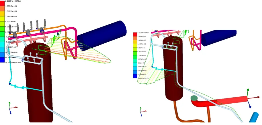
As example, seismic stress distribution in pressurizer pipeline system including potential dangerous zone is demonstrated on fig. 5. Natural vibration mode is demonstrated on fig. 6.

Figure 6. Seismic stress distribution for the pressurizer pipelines. General view and dangerous T-nozzle zone.

For the dangerous zones additional calculations on the base of exact normal mode method, the stress decreased to the below dangerous (212 MPa) level. Thus the normal mode method can be recommended for the result improvement in cases, when after spectral method obtained stresses are close to dangerous values.

CONCLUSION

The original variant of transfer matrix approach is presented for the simulation of harmonic vibrations of complex multibranched systems with taking into account vibration of internal fluid with the consideration of junction and Poisson coupling. The method uses exact expressions for beams with distributed mass and demonstrates analytical solution accuracy.

For the effective solution of transcendental eigenvalues problem the frequencies counter of Williams and Wittrick is implemented. To take into account fluid vibration the dynamic stiffness matrix, which is used by the counter, is extended: variable of the fluid displacement and correspondent equation of pressure balance are added. The special attention is paid for the matrix filling in T-nozzles and zones of pipe cross-section area change, where fluid displacement has a gap, unlike the mechanical pipe displacement. Special principle is developed to express additional fluid displacements on the base of neighbor parameters. Natural vibration modes are easily obtained by original “displacement disjunction method”, realized within transfer matrix approach, at that vibration displacements and forces are obtained in one iteration only for a given frequency.

The accuracy of natural frequency determination is demonstrated by the numerical tests and comparison with theoretical and experimental data.

Two variants of dynamic behavior modeling are demonstrated: theoretically exact normal mode method and response spectrum method, used for seismic analysis. The conclusion is drawn that normal mode method should be used for calculation result improvement in case of essential seismic stresses, obtained by spectral method.

any additional discretization of calculation model. The same model can be used for static and dynamic calculations, amount of the calculation elements is specified by the pipeline geometry and physical properties.

REFERENCES

Banerjee, J.R. and Williams, F.W. (1994). “Clamped-clamped natural frequencies of a bending-torsion coupled beam,”Journal of Sound and Vibration, 176(3), 301-306.

Batura, A.S., Bogdan, A.V., Orynyak, I.V. and Radchenko, S.A. (2014). “Two axisymmetric models application for fast and conservative analysis of cold plumes in RPV at PTS condition,” PVP2014-28997, Proceedings of the ASME 2014 Pressure Vessels & Piping Conference PVP2014, July 20-24, 2014, Anaheim, California, USA.

Dubyk I.R. and Orynyak I.V. (2016). “Fluid-structure interaction in free vibration analysis of pipelines,”

Scientific Journal of the Ternopil National Technical University, 1(81)

Moussou, P., Vaugrante, P., Guivarch, M., and Seligmann, D. (2000). “Coupling effects in a two elbows piping system,”Proc of 7th Int Conf on Flow Induced Vibrations, Lucerne, Switzerland, 579-586. Orynyak, I.V., Dubyk, I.R., Batura, A.S. (2015). “Energy approach for determine frequency and

amplitude of vibration of piping with closed side branches,” Proceedings of the ASME 2015 Pressure Vessels and Piping Conference PVP2015-45289, July 19-23, 2015, Boston.

Orynyak, I.V., Radchenko, S.A., and Batura, A.S. (2007). “Calculation of natural and forced vibrations of a piping system. Part 1. Analysis of vibrations of a 3D beam system,”Strength of Materials, 39(1), 53 – 63.

Orynyak, I.V., Torop, V.M., Romashchenko, V.A., and Zhurakhovskii, S.V. (1998) “Numerical Analysis of a Three-dimensional Branched Pipeline Using Special Software Designed for Estimation of the Strength of the Equipment of Nuclear Power Plants,”Strength of Materials, 30(2), 169-179.

PNAE G-7-002-86 (1987). “Rules of strength calculation for equipment and pipelines of nuclear power plants”

Wiggert, D.C. and Tijsseling, A.S. (2001). “Fluid transients and fluid-structure interaction in flexible liquid-filled piping,”Appl. Mech. Rev. 54, 455–481. doi:10.1115/1.1404122

Williams, F.W. and Wittrick, W.H. (1970). “An automatic computational procedure for calculating natural frequencies of skeletal structures,”Int. J. mech. Sci., Pergamon Press, 12, 781-791.

Williams, F.W. and Wittrick, W.H. (1983). “Exact Buckling and Frequency Calculations Surveyed,”

Journal of Structural Engineering, 109(1), 169–187.

Williams, F.W., Yuan, S., Ye, K., Kennedy, D. and Djoudi, M.S. (2002). “Towards deep and simple understanding of the transcendental eigenproblem of structural vibrations,” Journal of Sound and Vibration, 256(4), 681-693

Yuan, S., Ye, K., Williams, F.W., Kennedy, D. (2003). “Recursive second order convergence method for natural frequencies and modes when using dynamic sti ness matrices,”Int. J. Numer. Meth. Engng 2003, 56:1795–1814 (DOI: 10.1002/nme.640)