Analysis of Hypersonic Aircraft Inlets Using Flow Adaptive Mesh Algorithms

NEAVES, MICHAEL DEAN. Analysis of Hypersonic Aircraft Inlets Using Flow Adap-tive Mesh Algorithms. (Under the direction of D. Scott McRae.)

BIOGRAPHY

ACKNOWLEDGEMENTS

I would like to thank my advisor, Dr. McRae, for his support. I would also like to thank Dr. Fred DeJarnette, Dr. Hassan, and Dr. Edwards for being on my committee and teaching me on many occasions. Thanks to Dr. Scroggs and Dr. Vouk for being on my committee. I would like to thank Dr. Nd Chokani for standing in for Dr. Edwards during my oral preliminary examination. I thank the North Carolina Supercomputing Center for a grant of supercomputing resources and the Air Force Office of Scientific Research for various grants as overseen by Dr. Len Sakell. I am grateful to Kent Misegades of Compu-tational Engineering International for assistance and instruction on making large three-dimensional animations using Ensight.

TABLE OF CONTENTS

LIST OF TABLES v

LIST OF FIGURES vi

NOMENCLATURE vii

1. INTRODUCTION 1

2. OUTLINE OF NUMERICAL PROCEDURE 8

2.1 Development of a Time-Accurate Implicit Algorithm. . . 8

2.2 Development of Coupled Adaption Update Algorithm . . . 11

2.3 Adaptive Grid Algorithm . . . 17

2.3.1 Orthogonal Adaptive Grid Algorithm . . . 18

2.3.2 Weight Function . . . 21

3. RESULTS AND DISCUSSION 23

3.1 Riemann Problem . . . 23

3.1.1 Fixed-Grid Riemann Solutions . . . 24

3.1.1.1 Subiterations. . . 24

3.1.1.2 Relaxation Parameters . . . 25

3.1.1.3 Minmod Limiter. . . 25

3.1.1.4 Time Step Size . . . 26

3.1.2 Adaptive Riemann Problem . . . 27

3.1.3 Computational Efficiency and Accuracy . . . 28

3.2 Scramjet Inlet . . . 30

3.2.1 Three-Dimensional Inlet Steady Results . . . 30

3.2.2 Computational Time . . . 34

3.2.3 Three-Dimensional Inlet Unstart Calculations . . . 35

3.2.3.1 Exit Flap Induced Unstart . . . 35

3.2.3.2 Angle of Attack Unstart . . . 38

4. CONCLUSIONS 41

LIST OF TABLES

LIST OF FIGURES

Figure 1. Orthogonal Adaptation Process Near Boundaries. . . 46

Figure 2. Shock Tube Solution for Various Subiterations . . . 46

Figure 3. Shock and Contact Surface for Various Subiterations . . . 47

Figure 4. Unity Relaxation Factors . . . 47

Figure 5. Minmod Limiter . . . 48

Figure 6. Shock Tube Solutions with Various Time Steps . . . 48

Figure 7. Shock and Contact Surface for Various Time Steps . . . 49

Figure 8. Adapted versus Unadapted Shock Tube Results . . . 49

Figure 9. Adapted Cell Volume and Grid Speeds . . . 50

Figure 10. Dual-Mode Scramjet Inlet Model . . . 50

Figure 11. Unadapted Grid and Pressure Contours . . . 51

Figure 12. Adapted Grid and Pressure Contours . . . 51

Figure 13. Grid from Previous Adaptation Algorithm . . . 52

Figure 14. Mesh Near Inlet Boundary for Original (left) and Orthogonal (right) Mesh Algorithms. . . 52

Figure 15. Grid and Pressure Contours in Aft Inlet and Isolator (Centerline). 53 Figure 16. Centerline Pressure Compared to Experimental Results . . . 53

Figure 17. Centerline Pressure in Aft Inlet and Isolator Region . . . 54

Figure 18. Adapted 3-D Mesh Surfaces (i=30,j=40,k=28) . . . 54

Figure 19. Density Contours on Bottom Wall, Centerline and Selected i Surfaces . . . 55

Figure 20. Adapted Mesh on Bottom Wall, Centerline and Selected i Surfaces 55 Figure 21. Exit Flap Unstart (0.0 ms and 1.65 ms). . . 56

Figure 22. Exit Flap Unstart (2.47 ms and 4.26 ms). . . 57

Figure 23. Exit Flap Unstart (4.67 ms and 5.49 ms). . . 58

Figure 24. Exit Flap Inlet Unstart in Progress I (3-D view) . . . 59

Figure 25. Exit Flap Inlet Unstart in Progress II (3-D view). . . 59

Figure 26. Exit Flap Inlet Unstart after Upper Cowl Spillage (3-D view) . . . 60

Figure 27. Angle of Attack Unstart (0.137 ms) . . . 60

Figure 28. Angle of Attack Unstart (0.275 ms and 0.686 ms) . . . 61

Figure 29. Angle of Attack Unstart (1.37 ms and 2.06 ms) . . . 62

Figure 30. Angle of Attack Unstart (2.75 ms and 3.43 ms) . . . 63

NOMENCLATURE

E,F,G flux vectors

H enthalpy

J transformation Jacobian

P pressure

P,Q,R parametric space coordinates

Re Reynolds Number

U dependent variable vector

V volume

t time

u,v,w velocity components

x,y,z space coordinates

curvature weighting coefficient

finite difference operator

computational space coordinates

density

biasing coefficient

non-dimensional time

difference of adaption variables

weight function

implicit approximation parameter

implicit approximation parameter

Subscripts

i,j,k computational space coordinates

physical quantity

partial derivative with respect to time

partial derivative with respect to x,y,z

freestream quantity

o total quantity

1 strong conservation form

Superscripts

convective component of inviscid flux

inviscid component of flux

subiteration index

pressure component of inviscid flux

n current time level

unsteady contravariant

volume adaptation control

αc ∆ ξ η ζ, , ρ σk τ φ ω υ ϕ p t x y z, ,

Time-accurate simulations of complex three-dimensional flow fields about or through airframe components cannot, in general, be computed with short turnaround times. For example, simulating the response of a turbulent, three-dimensional inlet flow field to a freestream, engine compressor face, or combustor perturbation can often require excessive computational resources in terms of time and/or memory requirements. The number of grid points required to properly resolve large turbulent problems can easily exceed available memory. The large number of timesteps required by most explicit time accurate flow solvers can consume hundreds, if not thousands, of hours on a supercom-puter. A time accurate, implicit flow solver coupled with a solution adaptive grid algo-rithm could make inlet unstarts a more tractable problem.

Research to date shows computation of high-speed aircraft internal flow fields to require three-dimensional calculations. In 1993, Korte et al studied sidewall compression scramjet inlets in an inviscid parametric study.1 _{A Mach 4 swept-sidewall inlet was} para-metrically improved using inviscid dimensional calculations. A turbulent three-dimensional solution was then obtained for the optimized inlet. The resulting inlet flow field was found to be a complex three-dimensional structure with many multi-dimensional shock/shock and shock/boundary-layer interactions. The viscous solution revealed a large top-wall boundary layer separation on the optimal solution inviscid design.

calculations were turbulent, but only two-dimensional since the experimental model did not vary in width. Sakata concluded that the compression process is dominated by the strong viscous interactions between shock waves and the turbulent boundary layer. Com-paring computational and experimental results, their most important conclusions were that the two-dimensional calculations have a tendency to overestimate the pressure recovery and that to more precisely simulate the inlet’s performance, three-dimensional calculations are required.

Paynter and Mayer et al have written extensively on flow stability issues and

boundary layer interaction and no bleed could result in an non-wave propagation domi-nated inlet unstart. The flow in the throat is not one-dimensional, making correctly locat-ing and calculatlocat-ing the throat region difficult uslocat-ing inviscid analysis. Mayer and Paynter conclude that future work should include viscous calculations to include throat blockage effects and to investigate inlet unstarts caused by boundary layer separation.

Trexler et al have performed numerous experiments on hypersonic-type inlets in

the Mach 4 Blow Down Facility at NASA Langley.9,10 _{A Trexler Dual-Mode Scramjet} Inlet Model is used as the basis for much of the computation results that follow. Much of their work is aimed at determining the maximum back pressure an inlet can sustain before unstarting. Burning fuel raises inlet back pressure, so throttling the exit to raise back pres-sure is a proxy for burning fuel. The inlet stability determines maximum back prespres-sure which determines maximum fuel burn - i.e. maximum thrust the propulsion system can produce.

In 1995, Knight et al redesigned the NASA P2 hypersonic inlet.11 _{The original} P-series inlets intended to cancel a reflected shock via surface turning at a reflection point in order to achieve higher pressure recovery and a nearly constant static pressure at the throat. The inlets were originally designed using the Method of Characteristics and a boundary layer model to account for displacement thickness. Experimental results showed that the reflected shock was not canceled by the surface turning which led to the redesign by Knight et al using a Reynolds-averaged Navier-Stokes code (NPARC).

thickness from the available flow area. The displacement thickness approach ignores any three-dimensional effects and all inviscid/boundary layer interactions. Most of the remaining work has been time accurate, two-dimensional simulations - usually inviscid. Grid adaptation has been utilitized in two-dimensional unstart analysis performed by Ben-son and McRae12 _{using an explicit Reynolds-averaged Navier-Stokes flow solver. Given} the inherent three-dimensional nature of turbulence, quasi one-dimensional and two-dimensional analysis have been shown to over predict pressure recovery and ignore com-plex three-dimensional shock/boundary layer interactions; thus making them inadequate for analyzing three-dimensional turbulent flow fields. The goal of the present work is to extend solution dynamic grid adaptation unstart calculations to large three-dimensional turbulent flow fields.

When using dynamic grid adaptation to restrain computer memory and processing times, there are two fundamentally different approaches to dynamic grid adaptation: point movement and enrichment. When constrained by computer memory resources, enrich-ment may not be a viable option for large three dimensional problems due to the variable memory aspect of enrichment. Another problem regarding the enrichment of structured grids is the breakdown of the conveniently structured data set. Point movement maintains a constant maximum memory requirement and the structured data set lends itself to simple algorithm vectorization. For the large three-dimensional structured grids used in internal flow calculations, point movement was chosen as the best option for dynamic adaptation.

algorithm are required. The steady state flow solver merely sees the grid point movement as a perturbation to the solution and no solution update or further coupling with the flow solver is required. In essence, the unsteady transformation terms are neglected exactly as the unsteady flow terms are neglected in most steady state flow solvers.

If time accuracy is desired while performing point movement grid adaptation, more must be done to ensure temporal accuracy while moving grid points. Two approaches exist to maintain temporal accuracy while moving the mesh: coupled and decoupled. The coupled approach was previously used in one dimension by Klopfer and McRae13 _{for explicit solvers and by Orkwis and McRae}14 _{for implicit solvers. Benson and} McRae15 _{used the coupled approach to solve the chain rule form of the governing} equa-tions in two and three dimensions using an explicit form of MacCormack’s method. The decoupled approach was introduced by Benson and McRae15 _{and continued by Laflin.}16 _In the decoupled approach, the grid adaptation and solution update algorithms are completely independent of the flow solver algorithm. The decoupled approach can use any flow solver because mesh point movement and solution update to the new grid are independent of the flow solver. The decoupled approach has the advantage of being extremely porta-ble, but the disadvantage is a costly solution update calculation. For the present work, a coupled approach is taken to avoid the largest portion of the costly solution update. The penalty paid for using a coupled approach is a lack of portability.

should be capable of calculating inlet unstarts due to engine or freestream perturbations. Three advances are discussed, the first being the development of a time accurate implicit flow solver. Time accurate subiterations of Rai17 _{were added to the planar Gauss-Seidel} flow solver of Edwards.18 _{The second advance is an efficient coupling of the grid point} movement transformation to the flow solver in order to solve properly the unsteady trans-formation governing equations. Solving the unsteady transtrans-formation governing equations is achieved by including the grid movement terms directly in the numerical formulation of the unsteady, transformed equation system. The unsteady transformation terms are easily incorporated into the Low-Diffusion Flux Splitting of Edwards.19 _{Grid speed terms are} included in the contravariant velocities, and a pressure term is required to convert enthalpy in the upwind terms into the required energy term in the governing equations.

Lastly, a new point movement algorithm is developed which minimizes grid skew-ness near viscous boundaries in order to calculate turbulent boundary layers. The point movement algorithm of Benson and McRae15 _{has been modified to include orthogonality} factors which prevent excessive grid skewness. A stretching factor (area ratio) raised to the dot product of unit normals (orthogonality factor) is used to adjust point movement coefficients as required to maintain grid quality. The weight function used in the point movement algorithm is a linear combination of scaled gradients and curvature of the dependent variables.20

Trexler et al.10 _{Starting from an adapted steady solution, dynamic adaptation unstarts were} calculated. To best simulate the experiment, the rear ramp in the diffuser was moved up and the exit pressure adjusted. The diffuser is primarily subsonic, so moving the ramp and increasing exit pressure will send a pressure wave forward which unstarts the inlet. A freestream perturbation unstart due to an angle of attack perturbation is also calculated and presented. Finally, time-accurate simulations of the three-dimensional unstart process are presented.

2. OUTLINE OF NUMERICAL PROCEDURE

2.1 Development of a Time-Accurate Implicit Algorithm

A standard alternative to the long turnaround times of explicit flow solvers is to use an implicit flow solver with a less severe CFL21 _{(Courant, Friedrichs, and Lewy)} sta-bility requirement. Unfortunately, most implicit algorithms are implemented in a non-time-accurate manner for tractability and steady state convergence, and as a result the implicit algorithms contain approximate factorizations, explicit boundary conditions, relaxation, and linearization error, etc. The subiteration techniques of Rai17 _{can be used to} restore time accuracy while still taking advantage of simplifying approximations to the implicit operator. Adding the time-accurate subiterations to the existing implicit code of Edwards18 _{results in a time-accurate upwind relaxation method. The existing implicit code} employs a second order LDFSS(2)19 _{upwind discretization with planar Gauss-Seidel} algo-rithm for time advancement.

The subiteration techniques of Rai17 _{can be applied to the generic form of a system} of partial differential equations. For development, consider the two-dimensional Euler equations as written in equation 1,

(1) where the non-linear flux vectors are

. (2)

t

∂ ∂U

F U( )

+ = 0

F U( ) x

∂∂ E U( ) ∂y

∂

G U( ) +

An implicit approximation in time for the solution of equation 1 can be expressed as

(3)

where the parameters and are chosen to provide different schemes with

dif-fering accuracy. Considering as a subiteration index22_{, subtracting from both sides}

of equation 3 yields:

. (4)

Setting and results in the three-point backward scheme which is

second-order accurate in time. Linearizing around and substituting into equation 4

results in the following:

(5)

. (6)

Finally, divide by , the physical time step, and multiply by . An implicit

approximation in time for the solution of equation 1 can now be expressed as:

. (7)

∆t t

∂ ∂U

F U( )

+ ∆Un υ∆t

1+ϕ

---F U( n+1) +

≈ (υ–1)∆t

1+ϕ

---F U( )n ϕ 1+ϕ

---∆Un–1

ν 1

2

---– –ϕ

 

 _O(∆t2₎

O(∆t3)

+ +

+ =

υ ϕ

p Up

∆Up υ∆t

1+ϕ

---F U( p+1)

+ –(Up–Un) (υ–1)∆t

1+ϕ

---F U( )n ϕ 1+ϕ

---∆Un–1

+ +

=

υ = 1 ϕ = 1 2⁄

Up

F U( p+1) F U( )p U

∂∂ F U

p

( )∆Up O(∆t2)

+ +

=

I 2∆t 3

---U

∂∂ F U

p

( )

+ ∆Up - 2∆t

3

---F U( )p UP 4 3 ---Un

– 1

3 ---Un–1 +

– =

∆t_p 3 2⁄

I

∆t_p

---U

∂∂ F U( )p

+ ∆Up - F U( )p

3 2

---UP–2Un 1 2 ---Un–1 +

∆t_p

---–

2.2 Development of Coupled Adaption Update Algorithm

The coupling of a three-dimensional adaptive mesh algorithm to a time accurate upwind implicit solution algorithm is presented in this section. The goal is to couple the grid point movement and solution update more closely to the flow solver by solving the unsteady transformation governing equations using an implicit algorithm with grid move-ment included in the spatial upwinding. It is shown that the grid movemove-ment terms can be incorporated into any existing upwinding scheme which splits the inviscid flux into a con-vective and pressure contribution. The new coupled solution adaptive mesh algorithm is temporally accurate while only adding point movement and mesh speed calculation to the overall computational requirements.

The flow fields under consideration are governed by the three-dimensional com-pressible Navier-Stokes equations.

(8)

where U is the vector of conserved variables, and are the combined

invis-cid and viscous fluxes. In a curvilinear coordinate system defined by the unsteady

trans-formation , the Navier-Stokes

equations can be written as shown in equation 9. Multiplying by the Jacobian, J, and using the standard manipulation of the spacial terms into strong conservation law form results in equation 10.

∂U

∂t --- ∂E

∂x --- ∂F

∂y --- ∂G

∂z

---+ + + = 0

E F, G

(9)

(10)

In the present development, and represents the Jacobian

of the coordinate transformation; i.e. the volume of a finite volume cell. The grid move-ment terms in equation 10 can be incorporated as shown below:

. (11)

Now to recast in strong conservation form, combine the derivative terms and

note that .

(12)

Further simplifications can be made by the following:

(13)

(14)

(15)

∂U

∂τ

--- ∂U

∂ξ

---∂ξ

∂t --- ∂U

∂η

---∂η

∂t --- ∂U

∂ζ

---∂ζ

∂t --- ∂E

∂ξ

---∂ξ

∂x --- ∂E

∂η

---∂η

∂x --- ∂E

∂ζ

---∂ζ

∂x --- ∂F

∂ξ

---∂ξ

∂y --- ∂F

∂η

---∂η

∂y --- ∂F

∂ζ ---∂ζ ∂y ---∂G ∂ξ ---∂ξ ∂z --- ∂G

∂η

---∂η

∂z --- ∂G

∂ζ

---∂ζ

∂z

---+ + + + + + + + +

+ + + = 0

J∂---_∂τU J∂---_∂ξU∂ξ

∂t

--- J∂---_∂ηU∂η

∂t

--- J∂---_∂ζU∂ζ

∂t --- ∂

∂ξ

--- JE∂ξ_∂ x

--- JF∂ξ_∂ y

--- JG∂ξ_∂ z ---+ +     ∂ ∂η

--- JE∂η_∂ x

--- JF∂η_∂ y

--- JG∂η_∂ z ---+ +     ∂ ∂ζ

--- JE∂ζ_∂ x

--- JF∂ζ_∂ y

--- JG∂ζ_∂ z ---+ +     + + + + +

+ = 0

J≡∂(x y z, , ) ∂ ξ η ζ⁄ ( , , )

J∂---_∂τU U∂_∂τ---J ∂

∂ξ

--- JE∂ξ_∂ x

--- JF∂ξ_∂ y

--- JG∂ξ_∂ z

--- JU∂ξ_∂ t ---+ + +     ∂ ∂η

--- JE∂η_∂ x

--- JF∂η_∂ y

--- JG∂η_∂ z

--- JU∂η_∂ t ---+ + +     ∂ ∂ζ

--- JE∂ζ_∂ x

--- JF∂ζ_∂ y

--- JG∂ζ_∂ z

--- JU∂ζ_∂ t ---+ + +     + + +

+ = 0

τ

t = τ

∂(JU)

∂t --- ∂

∂ξ

--- JE∂ξ_∂ x

--- JF∂ξ_∂ y

--- JG∂ξ_∂ z

--- JU∂ξ_∂ t ---+ + +     ∂ ∂η

--- JE∂η_∂ x

--- JF∂η_∂ y

--- JG∂η_∂ z

--- JU∂η_∂ t ---+ + +     ∂ ∂ζ

--- JE∂ζ_∂ x

--- JF∂ζ_∂ y

--- JG∂ζ_∂ z

--- JU∂ζ_∂ t ---+ + +     + +

+ = 0

U₁ = JU

E₁ JE∂ξ_∂ x

--- JF∂ξ_∂ y

--- JG∂ξ_∂ z

--- JU∂ξ_∂ t

---+ + +

=

F₁ JE∂η_∂ x

--- JF∂η_∂ y

--- JG∂η_∂ z

--- JU∂η_∂ t

---+ + +

=

G₁ JE∂ζ_∂ x

--- _JF∂ζ

∂y

--- _JG∂ζ

∂z

--- _JU∂ζ

∂t

---+ + +

The final form of the governing unsteady transformation compressible Navier-Stokes equations is given by equation 16.

(16)

The grid speed terms arise from an unsteady transformation and

repre-sent the time rate of change in computational space of a point fixed in physical space. The physical grid speeds can be calculated with a second order one sided difference, for

exam-ple, . Noting that , we see

the metric grid speed terms can easily be calculated from the physical grid speed and met-rics as shown in equation 17.

(17) Comparing the vector of conserved variables and the convective portion of the inviscid flux vector to the new grid movement terms (equation 18), the grid movement terms modify to the convective velocity in the inviscid flux and thus, may be incorporated into an existing fixed mesh upwinding scheme. In a transformed system, the grid move-ment term becomes part of the contravariant velocity as shown below. Thus, the unsteady grid transformation term may be implemented as a velocity correction in an existing upwinding scheme. The difference in the energy equation term results in a pressure com-ponent being subtracted from the last equation to convert from enthalpy to energy.

∂U₁

∂t

--- ∂E1

∂x

--- ∂F1

∂y

--- ∂G1

∂z

---+ + + = 0

ξt, ,ηt ζt

( )

x_t ∂_∂x t --- 3x

n+1

4

– xn+xn–1 2∆t

---= = ξ_x ∂ξ_∂

x --- 1

J --- ∂y

∂η

---∂z

∂ζ

--- ∂z

∂η

---∂y

∂ζ ---–     = =

(18)

Now consider the general inviscid flux in the direction from a steady

transfor-mation written as a sum of a convective and pressure components:

(19) where

, (20)

. (21)

The steady contravariant velocity is given as

. (22)

Incorporating the term into the convective portion of the inviscid flux requires

calculating an unsteady transformation contravariant velocity, as follows:

. (23)

Using as defined in equation 17, the unsteady transformation contravariant

velocity may be further simplified: U ρ ρu ρv ρw e_o Ec , ρuˆ ρuuˆ ρvuˆ ρwuˆ ρHuˆ Uξ˜t

,

ρξ˜

t

ρuξ˜t

ρvξ˜t

ρwξ˜t

e_oξ˜t

= = =

ξ

EI1 Ec+Ep J∇ξ ρuˆE˜

c

J∇ξpE˜p +

= =

E˜c 1 u v w H

E˜p

, 0 ξ˜ x ξ˜ y ξ˜ z 0 = =

H 1_ρ--- e( _o+p) and ξ˜x y z t, , ,

ξx y z t, , ,

∇ξ

---= =

uˆ = ξ˜xu+ξ˜yv+ξ˜zw

Uξ˜t

uˆu t

uˆu t = ξ˜xu+ξ˜yv+ξ˜zw+ξ˜t

ξ˜

. (24) Now, consider the resulting unsteady transformation convective flux,

, (25)

which using the definition of contravariant velocity, and equation 25 above can

be written as

. (26)

With the exception of the energy term, the unsteady transformation convective flux

calculated with achieves the desired goal of including the grid speed terms in

the original fixed mesh upwinding formulation. Comparing the energy term in equation

26 to the desired term in equation 18, one is energy while the other is enthalpy, thus

they differ by a pressure term. To convert enthalpy to the desired energy term , a

pressure term must be subtracted from the energy term in the pressure component of

the upwinding. The resulting unsteady transformation pressure flux is as follows: uˆut = ξ˜x(u–xt) ξ+ ˜y(v–yt) ξ+ ˜z(w–zt)

Ecut J ∇ξ ρuˆ u t

E˜c J ∇ξ ρ ξ[˜x(u–xt) ξ+ ˜y(v–yt) ξ+ ˜z(w–zt)]E

˜c

= =

uˆ

Ecu t J∇ξ ρ ξ[˜x(u–xt) ξ+ ˜y(v–yt) ξ+ ˜z(w–zt)]

1 u v w H J∇ξ ρuˆ ρuˆu ρuˆv ρuˆw ρuˆH ρξ˜ t ρξ˜ tu ρξ˜ tv ρξ˜ tw ρξ˜ tH +                       = =

uˆut (Uξ_t)

e_oξ˜t

( )

e_oξ_t

( )

pξ_t

. (27)

In summary, to incorporate the unsteady transformation grid speed terms into an existing upwinding, the only changes required are to use an unsteady transformation con-travariant velocity (equation 25) and an unsteady transformation pressure flux (equation 27). The upwinding scheme chosen for the present work is the Low-Diffusion Flux-Split-ting (LDFSS) of Edwards.19

E_{u t}p J∇ξp 0

ξ˜

x

ξ˜

y

ξ˜

z

ξ˜ – t

J∇ξp

0

ξ˜

x

ξ˜

y

ξ˜

z

x_tξ˜x+ytξ˜y+ztξ˜z

2.3 Adaptive Grid Algorithm

2.3.1 Orthogonal Adaptive Grid Algorithm

An improved point movement algorithm for three-dimensional solution-adaptive gridding applications is proposed as an alternative to the center-of-mass formulation used

in earlier work.12,15,16,20,25,26 _{Likewise, adaptation is performed in parametric space,} essen-tially defining an interpolant for moving physical space grid points to their new locations. The original center-of-mass method, when applied within a parametric space, gives excel-lent adaptation to inviscid flow features when starting from uniform grids, but can result in excessive grid skewness and grid crossover when starting from the highly clustered grids required to resolve turbulent boundary layers. The original center-of-mass method is modified in two ways as follows. The diagonal nodes are ignored which allows formula-tion of center-of-mass partial differential equaformula-tions (equaformula-tions 28-30 with unity coeffi-cients), and orthogonality restoring coefficients are added in the non-adapting directions.

Defining the interpolation variables corresponding to the computational and

direc-tions as and , the new orthogonal center-of-mass partial differential equations of the

following form are approximately solved in parametric space to facilitate adaptation:

(28)

(29)

ξ η, ζ

p q, r

ξ ∂∂ ωP

p ∂ ξ ∂ ---    ∇η ∇ξ --- 

 2

ξ ∇ •∇η ξ ∇ ∇η ---η ∂∂ ωP

p ∂ η ∂ ---    ∇ζ ∇ξ --- 

 2

ξ ∇ •∇ζ ξ ∇ ∇ζ ---ζ ∂∂ ωP

p ∂ ζ ∂ ---   

+ + = 0

p interpolant; ξ direction

( )

∇ξ ∇η

--- 

 2

ξ ∇ •∇η ξ ∇ ∇η ---ξ ∂∂ ωq

q ∂ ξ ∂ ---    η ∂∂ ωq

q ∂ η ∂ ---    ∇ζ ∇η --- 

 2

η ∇ •∇ζ η ∇ ∇ζ ---ζ ∂∂ ωq

q ∂ ζ ∂ ---   

+ + = 0

q interpolant; η direction

(30)

In this, are the weight functions for the interpolants. The point

movement equations are discretized in a fixed parametric space using standard

central-dif-ference techniques, assuming that . The equations are then

updated by a point Gauss-Seidel or Jacobi iteration subject to a reflection boundary condi-tion and a final smoothing pass with coefficients set to unity. Adaptacondi-tion is performed every time step for unsteady calculations. Point movement is accomplished through a remapping procedure developed in earlier work15 _{and is performed relative to a fixed} back-ground mesh. The orthogonal center-of-mass partial differential equations have non-unity coefficients of some second-derivative terms. If the new orthogonality coefficients are set to unity, the algorithm reverts to center-of-mass partial differential equations with perfor-mance similar to the original center-of-mass formulation. Considering equation 28 above,

the first non-unity coefficient represents a stretching factor raised to an

orthogonality factor . These new coefficients act in the

non-adapt-ing directions to weight the point movement as required to maintain or restore acceptable orthogonality. The stretching factor is a cell face area ratio squared, which is much greater than unity for the highly stretched (high aspect ratio) cells required to resolve tur-bulent boundary layers. The orthogonality factor is the absolute value of the dot product of surface unit vectors. It is a skewness measure and varies between zero and unity.

∇ξ ∇ζ

--- 

 2

ξ ∇ •∇ζ ξ ∇ ∇ζ ---ξ ∂∂ ωr

r ∂ ξ ∂ ---    ∇η ∇ζ --- 

 2

η ∇ •∇ζ η ∇ ∇ζ ---η ∂∂ ωr

r ∂ η ∂ ---    ζ ∂∂ ωr

r ∂ ζ ∂ ---   

+ + = 0

r interpolant; ζ direction

( )

ωp q r, , p q r, ,

∇ξ = ∇η = ∇ζ = 1

∇η ∇ξ⁄

( )

ξ

∇ •∇η ⁄( ∇ξ ∇η)

Consider a highly stretched and highly skewed cell with a near-unity orthogonality factor and a very large coefficient. The large coefficient dominates the other adaptation direction’s coefficients and tends to restore orthogonality. The orthogonality restoring point movement algorithm’s behavior in parametric adaption space is illustrated in Figure 1, “Orthogonal Adaptation Process Near Boundaries”. The skewness shown in parametric space would be excessive when mapped back to physical space on a highly stretched mesh. Previous center-of-mass algorithms can easily produce this type of skewness near a boundary due to considering only weight functions. The grid is highly skewed at time 1 in the direction adjacent to a boundary. The stretching factor is very large and raised to

a near unity orthogonality factor which makes the coefficient much larger than the

coefficient. When the point under consideration at location 1 is moved in direction

sub-ject to a reflection boundary condition, the direction dominates, and the point moves to

location 2. The final result is a nearly orthogonal grid in parametric space which maps back to acceptable orthogonality in physical space. The new orthogonal procedure signif-icantly reduces skewness and crossover problems in viscous regions while maintaining high resolution in the capturing of inviscid flow features.

If the grid is nearly orthogonal, the orthogonality factor is near zero, and the result-ing coefficients are near unity regardless of stretchresult-ing factor, causresult-ing the adaption algo-rithm to revert to a center-of-mass partial differential equation with unity coefficients. As desired for nearly orthogonal cells, adaptation is allowed to proceed as a function of the weight functions. Likewise, when a cell’s stretching factor is near unity, the orthogonality factor is irrelevant, and the center-of-mass partial differential equation formulation is

η η

η ξ

ξ

returned. In summary, two conditions return a center-of-mass partial differential equation which allows adaptation unconstrained by orthogonality considerations: an orthogonal grid or a rhombus-type cell. If the grid is orthogonal, adaptation should be allowed to pro-ceed. Rhombus-type cells are indicative of grids in inviscid flow regions where skewness is allowable as it affords better grid alignment with inviscid features.

2.3.2 Weight Function

Mesh movement using the concept of a parametric space center-of-mass

calcula-tion, as developed by Benson and McRae12,15,25,26,27_{, first requires calculating a weight} func-tion for each adaptafunc-tion direcfunc-tion. The weight funcfunc-tion is constructed as a linear combination of gradients and/or curvature of the dependent variables. The gradient of a variable is calculated as a central-difference approximation of a first derivative, and the curvature is a second derivative approximation. The weight function is formed as a linear

superposition of the gradients and curvature where is a biasing coefficient, is the

magnitude of the curvature, is the magnitude of the gradient, is a curvature

weight-ing coefficient, and k indicates a given flow variable. The weight function is scaled by the freestream values of the dependent variable, u_k, to determine the relative importance of the

local flow consistent with the overall flow field.20 _{The velocity weight function is not} scaled by the freestream velocity due to the local velocity approaching zero in the

bound-ary layer and at stagnation points. The Jacobian raised to in the weight function

pro-vides control of minimum and maximum cell volumes while adapting.16

σk ϕk

φk αc

(31)

After the raw weight function is calculated as shown in 31, it is smoothed and sub-jected to a minimum and maximum limit. The smoothing and weight function limiting prevents over adaptation to strong features, adapting to minutiae, and evacuating uniform flow regions. The upper and lower limits for the weight function are specified as a multi-ple/fraction of the average weight function. The lower limit is set to control the maximum cell spacing in uniform flow regions, and the maximum limit is set to control the minimum cell spacing in regions of large weight functions.

ω σk(αcϕk+(1–αc)φk)

u_k

--- ×Jβ

k

∑

3. RESULTS AND DISCUSSION

3.1 Riemann Problem

3.1.1 Fixed-Grid Riemann Solutions

3.1.1.1 Subiterations

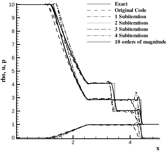
The first modification to the implicit code of Edwards is to add time accuracy improving subiterations. The time difference in equation 7 is added to the residual calcu-lation, a subiteration loop is added, and a global physical time step is specified. In order to evaluate the temporal accuracy of the subiterations on a fixed grid, the solutions using var-ious numbers of subiterations are compared to the exact solution. For comparison, the solution from the original code of Edwards is also plotted in Figure 2, “Shock Tube Solu-tion for Various SubiteraSolu-tions,” and Figure 3, “Shock and Contact Surface for Various Subiterations”. The locations of the contact surface and shock show the original algorithm has clearly lost time accuracy. The values of density and pressure are also incorrect. Time-accuracy errors in the original algorithm are expected due to linearization, factoriza-tion, and relaxation errors.

contact surface are captured well, and the shock speed error is less than one percent. For comparison, a solution was performed reducing each subiteration residual ten orders of magnitude, and the greater convergence provides no noticeable improvement over the three subiteration case.

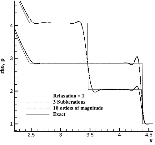
3.1.1.2 Relaxation Parameters

According to Matsuno23_{, a second order time-accurate scheme should require two} subiterations at most. Thus, even with a zeroth order initial guess, one should obtain sec-ond order accuracy after only two subiterations. Since each subiteration is rather compu-tationally expensive, minimizing subiterations is a driving concern in developing a practical time-accurate flow solver. Unfortunately, two subiterations do not seem to per-form admirably, as three subiterations were previously required to approach the more con-verged residual solution. The original code of Edwards has forward and backward sweep update relaxation parameters which are less than unity for optimal multigrid steady state convergence. When time accuracy is desired, all relaxation parameters should be set to unity. The results after setting all relaxation parameters to unity are presented in Figure 4, “Unity Relaxation Factors”. The results for two subiterations with the relaxation parame-ters set to unity are shown to be capable of producing results comparable to the solutions with many more subiterations.

3.1.1.3 Minmod Limiter

scheme. In an attempt to reduce oscillations near discontinuities, a Minmod limiter option was implemented. Figure 5, “Minmod Limiter,” shows the results of the Minmod limiter compared to the exact solution and the previous pressure based limiter results. The Min-mod limiter reduced or eliminated all oscillations. The resulting shock speed error is also reduced to about 0.7 percent.

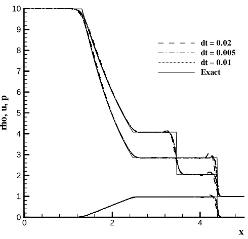
3.1.1.4 Time Step Size

In order to evaluate the new algorithm’s response to various physical time steps, additional solutions were calculated with CFL conditions corresponding to one half and two, time steps of 0.005 and 0.02 respectively. Figure 6, “Shock Tube Solutions with Var-ious Time Steps,” and Figure 7, “Shock and Contact Surface for VarVar-ious Time Steps,” showing the results compared to the previous baseline solution with a time step of 0.01, an explicit CFL of one. All calculations used two subiterations, relaxation parameters of one, and the Minmod limiter. The errors involved in a second order accurate in time scheme should be a function of the square of the time step.

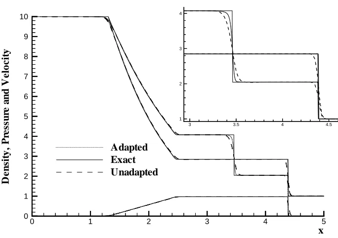
3.1.2 Adaptive Riemann Problem

Previous results showed the subiteration algorithm to be time accurate on a fixed grid. Dynamically adapting mesh shock tube calculations are required to verify the time accuracy of the unsteady grid movement terms which were incorporated into the upwind-ing scheme (LDFSS). The weight function for the adaptive grid calculations was calcu-lated with all biasing coefficients set to unity, a minimum limit of 0.1, and a maximum limit of 100. A curvature weighting coefficient of zero was used to allow adapting only to gradients which provided better resolution of the moving features. After smoothing of the weight function prior to use, the curvature contribution to the weight function tended to spread the weight function beyond the important features. The time step was 0.005 and the grid was adapted during every time step.

The shock tube solutions in Figure 8, “Adapted versus Unadapted Shock Tube Results,” show the flow solver algorithm to be time accurate for the adapted calculations. The shock speed error is less than half a percent and is mainly attributed to the initializa-tion error on a uniform grid. The adapted soluinitializa-tion is resolved much better, with the adapted normal shock being a nearly vertical line containing only three grid points. The contact surface shows less improvement from the unadapted to the adapted case due to dissipation added by the upwinding scheme to a moving contact surface. The added dissi-pation prevents the extra points provided by dynamic adaptation from more significantly sharpening the contact surface.

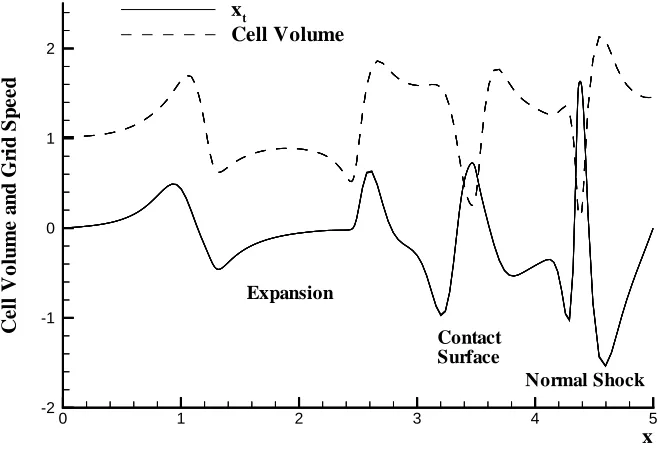
solu-tion. Near the normal shock, the grid speed is larger than the local fluid velocity. The expansion, contact surface, and normal shock can be clearly identified by the low cell vol-umes and higher grid speeds, indicating the movement of points into these regions as dic-tated by the weighting function. The minimum volume occurs at the normal shock and is about 13 percent of the original cell volume. The largest cells are only about twice the size of the original cells, and further point evacuation is undesirable for an unsteady prob-lem. Further point evacuation leads to excessive grid speeds when an unsteady feature moves into an evacuated region, and the excessive grid speeds can cause excessive disper-sion and/or dissipation.14

3.1.3 Computational Efficiency and Accuracy

The Riemann problem has an exact solution which can be compared to the adapted and fixed mesh solutions. The error vector is calculated as the difference between the primitive variable solution vector and the exact solution. The L2 Norm of the error vec-tors are calculated and shown are show in Table 1. The baseline case is a fixed mesh

solu-tion with 201 points in the X direcsolu-tion. For comparison, an adapted solusolu-tion and refined

Table 1: Error Norm and CPU Times for Riemann Problem

Case L2 Norm CPU Time (seconds)

201 points without adaptation 0.1538 319

201 points with adaptation 0.0659 322

401 points without adaptation 0.1200 636

3.2 Scramjet Inlet

3.2.1 Three-dimensional Inlet Steady Results

Steady solutions were obtained for a three-dimensional inlet/isolator component of a dual-mode scramjet geometry described by Emami et al.10 _{The experiments were} per-formed in the Mach 4 Blowdown Facility (M4BDF) at NASA Langley Research Center. Figure 10, “Dual-Mode Scramjet Inlet Model,” illustrates the geometry and sensor loca-tions of the experimental apparatus. Pressure data were collected along the bottom center-line and at the exit for various positions of the rear flap. The full open position of the rear flap corresponds to the 1.31 inch open position, and the closed position is at the 0.34 inch position. The steady calculations were performed with the rear flap in the 0.7 inch open position - the last position prior to the inlet unstarting in the experiment. The 0.7 inch open position case was chosen to locate the final shock near the exit of the isolator. The total inlet length is 32.7 inches with a sidewall beginning at 5.18 inches. The isolator extends from 9.77 inches to 13.25 inches. The original and adapted mesh steady solutions are presented, and the adapted mesh solution will be used as the initial solution for calcu-lating inlet unstarts. The calculation takes advantage of the symmetry about the centerline (k=33). The original mesh was used as the background grid for the adaptation process. The weight function was calculated with unity pressure biasing coefficients, 0.01 density

biasing coefficients in and , a minimum limit of 0.3, and a maximum limit of 7.0.

Turbulence closure is provided by a modified version of the Spalart-Allmaras model.25 The one-equation model is updated in a weakly-coupled manner after each iteration.

The solution on the original fixed mesh converged three and one half orders of magnitude. Judging convergence on a moving mesh calculation can be difficult due to the small perturbations from adaptation, so convergence of adaptive mesh solutions was judged by the centerline pressure trace. The convergence for an adapting grid calculation based on residual was only about one order of magnitude due to perturbations from solu-tion dynamic grid adaptasolu-tion. When allowed to converge on a fixed adapted grid, the residual dropped four orders of magnitude from the initial residual which is slightly more converged than on the original unadapted mesh.

The inlet geometry was represented by the original 325x81x33 mesh as shown in Figure 11, clustered to the walls to resolve turbulent boundary layers. Figure 11 presents pressure contours and mesh sections for constant-index surfaces (i=20, j=40, k=33) of the three-dimensional solution on the original unadapted mesh. The inlet ramp generates an initial oblique shock followed by a cowl shock which reflects into the isolator. The aft dif-fuser is a large subsonic region dominated by a large recirculation region. The pressure contours show the shocks and expansions entering the isolator to be poorly resolved fea-tures on the original grid.

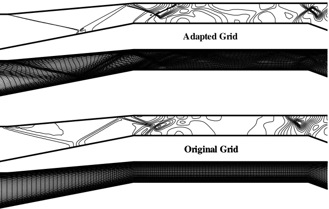
The orthogonal modifications to the adaption algorithm can be seen when com-pared to results from a previous version of the algorithm. No steady results from a previ-ous adaption algorithm are presented due to excessive grid skewness which induces flow solver instabilities. Figure 13, “Grid from Previous Adaptation Algorithm,” shows adap-tation from a previous version of the adapadap-tation algorithm. A very low level of adapadap-tation exists even at the initial strong oblique shock. The adaptation shown in Figure 13 results in the excessive skewness near a viscous boundary as shown in Figure 14, “Mesh Near Inlet Boundary for Original (left) and Orthogonal (right) Mesh Algorithms”. Figure 14 compares the adapted grid near the wall in the inlet region for the original and orthogonal mesh algorithms. The previous algorithm produces excessive skewness near the viscous boundary, and the excessive skewness impacts flow solver stability prior to achieving acceptable adaptation. By comparison, the orthogonal mesh algorithm results in a smooth, nearly orthogonal grid near the viscous wall.

The adapted mesh better resolves the shock at the exit of the isolator and locates it further aft than the original mesh.

Wall pressure distributions at the bottom wall centerline location are shown in Fig-ure 16. The magnitude of the pressFig-ure rise resulting from the cowl shock interaction with the bottom surface is predicted by both the adapted and unadapted mesh calculations. In the isolator shock reflections, the benefits of solution adaptation are seen more clearly, as the peak shock pressures are captured more precisely as shown in Figure 17. The adapted solution isolator exit shock location (x=13.25) is in better agreement with experimental results. The unadapted solution exit shock is too far forward and fails to detect the last expansion and shock as seen in the experimental data.

The three-dimensional nature of the solution adaptive mesh algorithm is illustrated in Figure 18, “Adapted 3-D Mesh Surfaces (i = 30, j = 40, k = 28)”. Inspecting the i and j surfaces reveals little in surface adaptation to the initial oblique shock, but the i and j sur-faces have adapted in such a way as to provide alignment with the initial oblique shock. The overall three-dimensional adaptation results in the initial oblique shock being resolved well as seen in the k surface. Aft of the i surface, the j surface mesh shows adap-tation to the weak shock arising from the sidewall. Following the j and k surfaces through the isolator reveals significant three-dimensional adaptation to even the weak features found in the isolator.

reveals two modes of adaptation: alignment from surface movement and reduction in grid spacing due to movement within a surface. Adaptation via alignment is more prevalent and desirable in inviscid regions and is best seen at the initial oblique shock location. The other i surfaces show more adaptation within the i surface. Adaptation within a surface is more dominant in viscous regions. The initial oblique shock has a spurious reflection off the upper boundary which is resolved and visible in the centerline plane and the second i surface. The upper cowl surface shock can be seen in the centerline plane and the third i surface. The train of weakening reflected shocks can been seen in the centerline plane. The final three i surfaces are aft of the sidewall location, and three-dimensional effects are noticeable near the wall. The i surfaces show distortions in the reflected shock train near the sidewall due to vortex and separation regions.

3.2.2 Computational Time

between computational time and errors resulting from a large time step. Exceeding the inviscid CFL of unity condition results in higher subiteration residuals, and thus provides feedback for proper time step choice. The relative speed up when using time accurate sub-iterations is problem and error tolerance dependent.

Previously, the adaptation algorithm overhead for the shock tube problem was noted to be around one percent on a CRAY T90. The three-dimensional inlet calculations were preformed on a Compaq DEC Alpha. A two subiteration time step without adapta-tion requires approximately 77 seconds, versus 80 seconds with adaptaadapta-tion. Thus, the adaptation algorithm’s overhead for the inlet under consideration is about 4 percent.

3.2.3 Three-Dimensional Inlet Unstart Calculations

3.2.3.1 Exit Flap Induced Unstart

A close up of the centerplane isolator with velocity vectors is also included. To enhance visibility, only every other velocity vector is shown.

A separation region has developed on the cowl which is also moving forward. Figure 25, “Exit Flap Inlet Unstart in Progress II (3-D view),” shows the shock surfaces being lifted and pushed forward ahead of the separation regions. At 4.67 ms (Figure 23) the unstart is accelerating as the shock structures being pushed forward by the separation regions are growing to fill the available flow area. The unstart is nearing upper cowl spillage at time 5.49 ms. Figure 26, “Exit Flap Inlet Unstart after Upper Cowl Spillage (3-D view),” shows the final three-dimensional shock structure. A large oblique shock is located out-side the cowl and ahead of a large recirculation region. A supersonic jet exists down the center of the isolator, as seen in the small diamond shocks in the center of the isolator. A region of reverse flow exists between the supersonic jet and the sidewall in the isolator. The unstart takes approximately 5.74 milliseconds from initiation to upper cowl spillage. After upper cowl spillage, the inlet is considered to be unstarted. Exit pressure drops sig-nificantly due to the reduced efficiency of the inlet shock system.

shock/boundary layer interactions appear to accelerate the unstart and have a deleterious effect on inlet stability.

3.2.3.2 Angle of Attack Unstart

Although no freestream perturbation experimental data exist for the geometry under consideration, an angle of attack unstart was calculated as a code demonstration exercise. The inlet was subjected to an angle of attack perturbation of 10 degrees ramped over 0.02 ms. The steady, adapted solution previously discussed is used as an initial con-dition. The perturbation and resulting unstart is predominately a result of the inlet and iso-lator disturbances.

continues to strengthen and has now formed a separation region. The aft cowl and isolator flow fields now consist of an oblique shock train with few distinct features.

Figure 30 shows the final stages of the unstart. At 2.75 ms, the first shock reflec-tions on the inlet and cowl have decoupled from the isolator flow field. The separation region behind the cowl shock/boundary layer interaction has grown to fill approximately half the flow channel and is rapidly expelling the shock structure. The reflected shock separation region on the cowl is also growing but appears secondary as an unstart mecha-nism. At 3.43 ms the driving separation has nearly filled the available flow area, and the shock generated by the separation region is rapidly moving toward the upper cowl lip. By 4.12 ms (Figure 31), the inlet has upper cowl spillage and is considered to have unstarted. The flow field is dominated by the large recirculation region on the lower surface of the inlet, the shock created by the recirculation region, and several normal or near-normal shocks in the cowl and isolator regions. In the unstarted condition, pressure recovery is severely impacted by the normal shocks, and the inlet/engine assembly would provide lit-tle thrust until the inlet is restarted.

4. CONCLUSIONS

5. References

[1] Korte, J.J., Singh, D.J., Kumar, A., and Auslender, A.H., 1993, “Numerical Study of the Performance of Swept, Curved Compression Surface Scramjet Inlets,” AIAA Paper 93-1837.

[2] Sakata, K., Yanagi, R., Murakami, A., Shindo, S., Honami, S., Shizawa, T., Sakamoto, K., Shiraishi, K., and Omi, J., 1993, “An Experimental Study of Supersonic Air-Intake with 5-Shock System at Mach 3,” AIAA Paper 93-2305.

[3] Omi, J., Shiraishi, K., Sakata, K., Murakami, A., Honami, S., and Shigematsu, J., 1993, “Two-Dimensional Numerical Simulation for Mach-3 Multishock Air-Intake with Bleed Sys-tems,” AIAA Paper 93-2306.

[4] Paynter, G.C., Mayer, D.W., and Tjonneland, E., 1993, “Flow Stability Issues in Supersonic Inlet Flow Analyses,” AIAA Paper 93-0290.

[5] Mayer, D.W., and Paynter, G.C., 1993, “Boundary Conditions for Unsteady Supersonic Inlet Analyses,” International Symposium on Air Breathing Engines, Sept. 20-24, 1993, Tokyo, Japan.

[6] Mayer, D.W., and Paynter, G.C., 1994, “Prediction of Supersonic Inlet Unstart Caused by Freestream Disturbances,” AIAA Paper 94-0580.

[7] Decher, R., Mayer, D.W., and Paynter, G.C., 1994, “On Supersonic Inlet-Engine Stability,” AIAA Paper 94-3371.

[8] Mayer, D.W., and Paynter, G.C., 1995, “Prediction of Supersonic Inlet Unstart Caused by Freestream Disturbances,” AIAA Journal, Vol 33, No. 2, Pages 266-275, February 1995.

[9] Emani, S., Rodi, P.E., Trexler, C.A., and Beaulieu, W., 1995, “Analysis of Time Accurate Pressure Measurements in a Ramjet/Scramjet Inlet Configuration,” AIAA Paper 95-0037.

[10] Emami, S., Trexler, C.A., Auslender, A.H., and Weidner, J.P., “Experimental Investigation of Inlet-Combustor Isolators for a Dual-Mode Scramjet at a Mach Number of 4,” NASA TP 3502, Langley, VA, 1995.

[11] Gelsey, A., Knight, D.D., Gao, S., and Schwabecher, M., 1995, “NPARC Simulation and Redesign of the NASA P2 Hypersonic Inlet,” 31st AIAA Joint Propulsion Conference, San Diego, CA, July.

[12] Benson, R.A., and McRae, D.S., 1993, “Numerical Simulations of the Unstart Phenomena in a Supersonic Inlet/Diffuser,” AIAA Paper 93-2239.

[14] Orkwis, P.D., and McRae, D.S., 1987, “Analysis of Standard Implicit Schemes with Arbi-trary Mesh Movement,” AIAA 87-1171.

[15] Benson, R.A., and McRae, D.S., 1990, “A Three-Dimensional Dynamic Solution-Adaptive Mesh Algorithm,” AIAA Paper 90-1566.

[16] Laflin, K.R., 1997, “Solver-Independent r-Refinement Adaption for Dynamic Numerical Simulations,” Ph.D. Dissertation, North Carolina State University, 1997.

[17] Rai, M.M., 1987, “Navier-Stokes Simulations of Blade-Vortex Interaction Using High-Order Accurate Upwind Schemes,” AIAA Paper 87-0543.

[18] Edwards, J.R., 1995, “Development of an Upwind Relaxation Multigrid Method for Com-puting Three-Dimensional, Viscous Internal Flows,” AIAA Paper 95-0208.

[19] Edwards, J.R., 1997, “A Low-Diffusion Flux-Splitting Scheme for Navier-Stokes Calcula-tions,” Computers & Fluids, Vol. 26, No. 6, pp.635-659.

[20] Neaves, M.D., and McRae, D.S., 1995, “Numerical Investigation of the Unstart Phenome-non in an Axisymmetric Supersonic Inlet,” Proceedings of the 1995 ASME International

Mechan-ical Engineering Congress & Exposition.

[21] Courant, R., Friedrichs, K.O., and Lewy, H., 1967, “On the Partial Difference Equations of Mathematical Physics,” IBM Journal of Research and Development , vol. 11, pp. 215-234.

[22] Pulliam, T.H., “Time Accuracy and the Use of Implicit Methods,” AIAA Paper 93-3360, 1993.

[23] Matsuno, K., “Higher-Order Time-Accurate Scheme for Unsteady, Three-Dimensional Flows,” AIAA Paper 93-3362, 1993.

[24] Eiseman, P.R., 1987, “Adaptive Grid Generation,” Computational Methods Applied Mechanical Engineering 64, p. 321.

[25] Benson, R.A., McRae, D.S., and Edwards, J.R., 1992, “Numerical Simulations Using a Dynamic Solution-Adaptive Grid Algorithm, with Applications to Unsteady Internal Flows,” AIAA Paper 92-2719.

[26] Benson, R.A., 1989, “A Dynamic Solution-Adaptive Grid Algorithm in Two and Three Dimensions,” Master’s Thesis, North Carolina State University, Raleigh, NC.

[27] Benson, R.A., and McRae, D.S., 1991, “A Solution-Adaptive Mesh Algorithm for Dynamic/Static Refinement of Two and Three Dimensional Grids,” Proceedings of the Third

International Conference on Numerical Grid Generation in Computational Fluid Dynamics and Related Fields, A.S. -Arcilla et al., ed., North -Holland Publishing Company, Amsterdam, The

FIGURE 1. Orthogonal Adaptation Process Near Boundaries

η

ξ

2 4

x 0

1 2 3 4 5 6 7 8 9 10

rh

o

,

u

,

p

Exact Original Code 1 Subiteration 2 Subiterations 3 Subiterations 4 Subiterations 10 orders of magnitude

2.5 3 3.5 4 4.5

x

1 2 3 4

rh

o

,

p

Exact Original Code 1 Subiteration 2 Subiterations 3 Subiterations 4 Subiterations 10 orders of magnitude

FIGURE 3. Shock and Contact Surface for Various Subiterations

2.5 3 3.5 4 4.5

x

1 2 3 4

rh

o

,

p

Relaxation = 1 3 Subiterations 10 orders of magnitude Exact

2.5 3 3.5 4 4.5

x

1 2 3 4

rh

o

,

p

Exact Relaxation = 1 Minmod

FIGURE 5. Minmod Limiter

0 2 4

x

0 1 2 3 4 5 6 7 8 9 10

rh

o

,

u

,

p

dt = 0.02 dt = 0.005 dt = 0.01 Exact

2.5 3 3.5 4 4.5 x 1 2 3 4 rh o , p

dt = 0.02 dt = 0.005 dt = 0.01 Exact

FIGURE 7. Shock and Contact Surface for Various Time Steps

3 3.5 4 4.5

1 2 3 4

0 1 2 3 4 5

x 0 1 2 3 4 5 6 7 8 9 10 D e n si ty , P re ss u re a n d V e lo c it y Adapted Exact Unadapted

0 1 2 3 4 5

x

-2 -1 0 1 2

C

e

ll

V

o

lu

m

e

a

n

d

G

ri

d

S

p

e

e

d

x_t

Cell Volume

Expansion

Contact Surface

Normal Shock

FIGURE 9. Adapted Cell Volume and Grid Speeds

i = 20

j = 40

k = 33 i = 20

j = 40

k = 33

FIGURE 11. Unadapted Grid and Pressure Contours

FIGURE 12. Adapted Grid and Pressure Contours

i = 20

j = 40

k = 33 i = 20

j = 40

FIGURE 13. Grid from Previous Adaptation Algorithm

Original Grid Adapted Grid

Original Grid

FIGURE 15. Grid and Pressure Contours in Aft Inlet and Isolator (Centerline)

0 10 20 30

x

5 10 15 20

P

re

ss

u

re

Adapted Grid Original Grid Experimental

7 8 9 10 11 12 13 14

x

5 10 15

P

re

ss

u

re

Adapted Grid Original Grid Experimental

FIGURE 17. Centerline Pressure in Aft Inlet and Isolator Region

0 10

0.5 0

1 2

X Y

Z

0 10

0.5 0 1 2

Z X

Y

FIGURE 19. Density Contours on Bottom Wall, Centerline and Selected i Surfaces

0

10

0.5

0

1

2

Z X

Y

Time = 0.0 ms k = 33

k = 33 j = 40

k = 33

j = 40

Time = 1.65 ms

k = 33

Time = 2.47 ms

k = 33

k = 33

j = 40

k = 33 j = 40

Time = 4.26 ms k = 33

Time = 4.67 ms k = 33

k = 33 j = 40

k = 33

j = 40

Time = 5.49 ms

k = 33

FIGURE 24. Exit Flap Inlet Unstart in Progress I (3-D view)

FIGURE 26. Exit Flap Inlet Unstart after Upper Cowl Spillage (3-D view)

Time = 0.137 ms k = 33

k = 33 j = 40

k = 33

j = 40

Time = 0.275 ms

k = 33

Time = 0.686 ms

k = 33

k = 33

j = 40

k = 33 j = 40

Time = 1.37 ms k = 33

Time = 2.06 ms k = 33

k = 33 j = 40

k = 33 j = 40

Time = 2.75 ms k = 33

Time = 3.43 ms

k = 33

k = 33

j = 40

k = 33

j = 40

Time = 4.12 ms

k = 33