The fluency effect as the underlying variable for judging beauty and usability

(1)

UNIVERSITY OF TWENTE

MASTER THESIS

The fluency effect as the underlying

variable for judging beauty and

usability

Author: Deniece S. Nazareth

(2)

(3)

Abstract

(4)

(5)

(6)

(7)

List of Figures

Figure 1. Inference perspective extended by Hassenzahl and Monk (2010). ... 4

Figure 2. Information-processing stage model by Leder et al.(2004)... 7

Figure 3. Affect heuristic as a mediator in processing fluency and judgment. ... 12

Figure 4. Causes and consequences of Fluency. (Left : Kahneman, 2011, Right: Weiss-Lijn, 2012). ... 12

Figure 5. The fluency model. ... 15

Figure 6. Visualization of the randomization and selection of stimuli. ... 20

Figure 7. Procedure of the experiment. ... 23

Figure 8. Reaction time of questionnaire against age. ... 26

Figure 9. Reaction time of viewing the stimuli against age. ... 27

Figure 10. Regression estimates of the model. ... 29

Figure 11. Boxplot of repeated exposure. ... 30

Figure 12. Interaction plot of PT and scale. ... 32

Figure 13. Interaction plot of VS and scale. ... 33

Figure 14. Interaction plot of PT and condition. ... 35

Figure 15. 2-way interaction plot of PT and condition between the three scales. ... 36

Figure 16. Interaction plot of VS and condition. ... 37

Figure 17. 2-way interaction plot of VC and condition for the three scales. ... 38

Figure 18. Boxplot of the reaction time of answering the questions and condition. ... 40

Figure 19. Boxplot of the reaction time when viewing the stimuli and condition. ... 42

(11)

List of Tables

Table 1 An overview of studies examining the relation beauty-usability ... 3

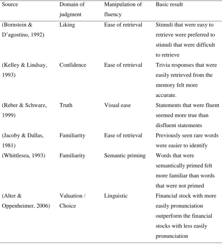
Table 2 An overview of the fluency effect in different domains of judgment... 10

Table 3 Estimated fixed effects coefficients, with alpha error and 95% credible intervals ... 28

Table 4 Pearson correlation between scales in the conditions ... 39

Table 5 Parameter estimates and estimated marginal means of reaction time when answering the questions ... 41

(12)

(13)

(14)

(15)

(16)

information that is unavailable at the time. Their inference model proposes that the starting point of these inference processes is beauty, as its nature is primarily sensory therefore immediate available (Hassenzahl & Monk, 2010).

.

Figure 1. Inference perspective extended by Hassenzahl and Monk (2010).

(17)

(18)

(19)

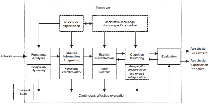
information can be processed due to lack of time, information is not inferred, information is just processed in lower stages than it would otherwise.

Figure 2. Information-processing stage model by Leder et al.(2004).

(20)

(21)

(22)

(23)

(24)

Stimuli Fluency (feeling of

ease) Affect impression Higher judgments

Figure 3. Affect heuristic as a mediator in processing fluency and judgment.

Thus, the fluency effect results in more positive feelings when judging stimuli. Figure 4 shows different feelings of judgments when the stimulus is processed fluently. Ergo, the conclusion can be made that fluency has an uniform positive effect across different domains of judgments (Alter & Oppenheimer, 2009). However, to the best of our knowledge, not a lot of research has been conducted regarding usability judgment and processing fluency. Van Rompay, de Vries and van Venrooij (2010) discussed that the impression of enhanced website usability of a user may be the result of fluent processing. The relationship of beauty and perceived usability however, leads to our proposal of explaining perceived usability and perceived beauty by processing fluency.

(25)

(26)

(27)

(28)

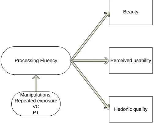
„why‟ of interaction (Hassenzahl & Monk, 2010). It subjectively measures the quality as perceived by the user (e.g. innovative or originality), without a direct connection to the goals that are related to the tasks (Hassenzahl & Monk, 2010). For users, it is important that they perceive the product in the same way as the designers in order for a product to be usable. So, based on these results, hedonic quality was added to the model in order to test it. If processing fluency is true, it will affect all scales.

Furthermore, Figure 5 shows the relevant manipulations of the fluency model for this study. As discussed earlier, repeated exposure, VC and PT will be used to manipulate fluency in order to examine if processing fluency is the underlying variable. As processing fluency influences judgment of perceived beauty positively, the expectation is that high fluency will lead to a more positive judgment of beauty. This study expects that, besides perceived beauty, the judgment of perceived usability and hedonic quality will also be more positive as processing fluency will influence all factors.

Therefore, the research question of this study is: Is processing fluency the cognitive process of perceived beauty, perceived usability and hedonic quality?

The hypotheses that will support the research questions are:

H1. High fluency due to repeated exposure will lead to a more positive judgment of perceived

beauty, perceived usability and hedonic quality.

H2. High fluency due to low VC will lead to a more positive judgment of perceived beauty,

perceived usability and hedonic quality.

H3. High fluency due to high PT will lead to a more positive judgment of perceived beauty

perceived usability and hedonic quality.

(29)

(30)

(31)

(32)

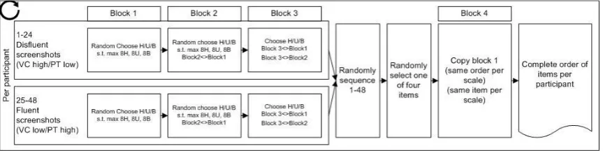
in the blocks (H-U-B, B-U-H, U-H-B, U-B-H, B-H-U, and H-B-U). One of the six combinations was then selected for each participant per screenshot. See Figure 6 for an illustration of the randomization and selection of the stimuli in the experiment. The random selection of items of each scale was not balanced out, resulting in some questions appearing more often than other questions of a scale (See appendix 6.6).

Figure 6. Visualization of the randomization and selection of stimuli. 2.3 Websites rated

In the current study, the websites in the study of Tuch et al. (2012a) were. In the experiment, 48 American companies‟ websites were selected from the pool used in the study by Tuch et al. (2012b). The websites were chosen from the categories VC low – PT high (20 websites: high fluency) and VC high – PT low (20 websites: low fluency). Furthermore, eight websites were added in order to balance out the three scales more evenly. Analyzing their results, these websites had a VC low-PT high score or VC high-PT low score despite categorized in another group (e.g. VC medium, PT low) (Tuch et al., 2012a). For the practice phase, four new companies‟ websites were used to avoid priming or repeated exposure in the experiment phase. The companies‟ websites were selected from Tuch et al. (2012a) study. See appendix 6.8 for an overview of all websites.

2.4 Measures

(33)

(34)

(35)

Figure 7. Procedure of the experiment. 2.9 Data analysis

All data of the participants were used to analyze. Statistical programs IBM SPSS 21.0 and R were used to analyze the data (R Core Team, 2013; SPSS IBM, NY).

In R, the libraries LME4 (mixed effects models) (Bates, Maehler, Bolker, & Walker, 2014) and MCMCglmm (Markov chain Monte Carlo Generalized Linear Mixed Models) (Hadfield, 2009) were used.

(36)

Havinga, 2013). The Gaussian error term was used for the data model. For testing the hypotheses, we focused on the fixed effects results. The syntax of R can be found in appendix 6.4.

To examine whether the correlation between beauty and perceived usability would decrease after treatment, a bivariate correlation analysis was conducted in SPSS (see appendix 6.9 for the SPSS syntax).

(37)

3. Results

In total, 8064 responses were measured with 192 responses per participant. For the MCMC glmm analysis, the z-standardized scores of the response, VC and PT were used. The variable VC was transformed into visual simplicity (VS) for easier interpretation (Schmettow & Boom, 2013). The reference group consists of the hedonic quality scale, control condition and block 1. Several models were tested and the less complex model with a lower DIC (27629.75) was chosen. The main effects were VS, PT and blocks whereas the two-way interaction effects were VS*condition, VS*PT and PT*condition. Two three-way interaction effects were introduced in the model. They were VS*condition*scale and PT*condition*scale. The estimated fixed-effects coefficients are shown in Table 1. For treatment contrasts, the reference groups consisted of the control condition, the hedonic quality scale and the first block. The hedonic quality scale was used as the reference group as the study was targeted at the association between beauty and usability.

For the correlation analyses of the rating scales, the data consisted only of block 1 thus resulting in 1008 responses of the 48 screenshots per condition (21 participants per condition).

(38)

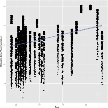
Plotting both reactions times against age, it appears that the time spent on viewing the stimuli and answering the questions, increased with age (Figure 8 and 9).

Figure 8. Reaction time of questionnaire against age.

(39)

(40)

(41)

Figure 10. Regression estimates of the model. 3.1 The fluency effect

The research question was whether processing fluency is the underlying variable of perceived beauty, perceived usability and hedonic quality. As we expected that repeated exposure, VC and PT would lead to more positive judgments of these three constructs, they will now be discussed.

3.1.1 Scale

(42)

3.1.2 Repeated exposure

Figure 11 displays the plot for repeated exposure. It appears that Block 2 and 3 had higher responses than Block 1 and fourth. It was expected that Block 4 would be in line with Block 2 and 3, therefore it is a surprising result.

Figure 11. Boxplot of repeated exposure.

(43)

3.1.3 Prototypicality

(44)

Figure 12. Interaction plot of PT and scale. 3.1.4 Visual Complexity

(45)

not differ much compared to the hedonic quality scale but resulted still in slightly more positive judgments when the websites are visually simple (Δresponse=.051).

Figure 13. Interaction plot of VS and scale.

3.1.5 Interaction between visual complexity and prototypicality

Table 3 shows that a significant interaction effect was found between VS and PT (Δresponse =.358, p=.022). This means that websites that are visual simple and high in prototypicality results in more positive judgments.

3.2 Breaking the fluency effect

(46)

analyzed. Furthermore, two three-way interaction were introduced in the model, namely VS*condition*scale and PT*condition*scale. Also, we hypothesized that the correlation between beauty and perceived usability would decrease in the treatment condition.

Lastly, we expected that the reaction time in the treatment would be longer than in the control condition due to the activation of System 2.

3.2.1 Treatment condition

In order to answer the hypothesis of breaking fluency, we will take a look at the treatment condition. The expectation is that the effect of fluency is gone in the treatment condition, resulting in less positive judgments on the scales. This would mean that the judgments on the beauty, perceived usability and hedonic quality scales are more “true”.

Based on Table 3, the treatment condition was judged less positive in comparison with the control condition (Δresponse=-.235) although it did not met statistical significance.

3.2.2 Prototypicality and treatment

(47)

Figure 14. Interaction plot of PT and condition.

Analyzing Table 3, the interaction effect is indeed found which met statistical significance (Δresponse=0.155, p=.034). Thus, the effect of PT differs between the control and treatment condition. However, in contrast with Figure 14, the result suggests that the treatment condition leads to more positive judgments in comparison with the control condition. To see whether the effect of PT and condition differs among the three scales, a 3-way interaction effect is conducted (Figure 15).

(48)

interaction for the hedonic quality scale (Δresponse=-.247). In comparison with the hedonic quality scale, the judgments of PT in the treatment condition were less positive for perceived usability (Δresponse=-.203). For the perceived usability scale, no significant 3-way interaction was found.

Figure 15. 2-way interaction plot of PT and condition between the three scales.

3.2.3 Visual simplicity and treatment

(49)

are almost the same in the treatment and control condition. Visual complex websites are perhaps processed less fluent (more cognitive restrain), thus disfluency can occur which explain the similar results of the treatment and control condition. Looking at Table 3, there is indeed an interaction effect between VS and condition. The judgments are less positive in visual simple websites in the treatment condition, in comparison with the control condition (Δresponse=-.217). The interaction effect between VS and condition reached statistical significance (p=.004). This result supports the breaking fluency hypothesis.

(50)

Figure 17 illustrates the three-way interaction effect of VS, condition and scales. It seems that the three-way interaction effect differs at the different scales. Table 3 shows if the interaction effect of VS and condition indeed differs between scales. For the perceived beauty scale, the interaction effect of VS and condition was found significant (p=.010). In comparison with the hedonic quality scale interaction effect, the judgments on the beauty scale were more positive on visual simple websites in the treatment condition (Δresponse=.256) However, this effect is almost cancelled out when compared to the interaction effect VS and condition on the hedonic quality scale. The interaction effect did not reach statistical significance on the perceived usability scale and the judgments were a bit more positive in comparison with the hedonic quality scale (Δresponse=.102).

(51)

(52)

(53)

Table 5

Parameter estimates and estimated marginal means of reaction time when answering the

questions

Parameter Β SEβ Wald‟s χ2 df p

Intercept 8.159 .0820 9893.61

1

1 .000

Control .040 .1271 .098 1 .754

Treatment 0

Scale 0.676

Estimated marginal means

Moderated M SE

Control 8.199 .097

Treatment 8.159 .082

Looking at Table 5, the reaction time in the control condition is slightly higher. This means that participants in the control condition took longer to answer the questions in comparison with the treatment condition (β= .040). It did not meet statistical significance. However, the difference is minimal as we can see in the estimated marginal means for the control condition (M=8.199) and treatment condition (M=8.159).

Reaction time for viewing the stimuli

(54)

(55)

(56)

(57)

(58)

(59)

(60)

(61)

(62)

(63)

(64)

(65)

(66)

(67)

(68)

(69)

(70)

had a longer preparation time when the recipe had a fancier font which made it harder to read. The fancier font was thus processed more strained, resulting in the substitution of the target question “How long the dish takes to prepare” by the heuristic question “Is it hard to read the recipe?” (Song & Schwarz, 2008). Regarding the attribute substitution of beauty and perceived usability, this would translate in the fluency of the features that influences beauty (e.g. symmetry, color) mediates the substitution. Another possibility of the two models working together is that the fluency model would address to different errors in judgments in System 1, whereas attribution substitution could account for errors in judgments when System 1 and System 2 are joint. These are of course assumptions as no evidence is found as of today. Therefore, it would be good and interesting to test the model. This would not only lead to a better and possible different understanding of beauty and perceived usability, but it would also analyze how the fluency model interacts (i.e. fits) with the attribution substitution assuming of course that they do not exclude each other.

(71)

(72)

(73)

(74)

(75)

(76)

(77)

6. Appendix

6.1 Treatment criteria list

CRITERIA LIJST

SCHOONHEID

Maak een lijst van 5 woorden die voor u een criteria zijn voor Schoonheid (Beauty). Dit zijn woorden waarmee u Schoonheid definieert. Deze woorden mogen niet hetzelfde zijn als de woorden in de Gebruiksvriendelijkheid (usability) lijst hieronder.

1. ……….……….

2. ……….……….

3. ……….……….

4. ……….……….

5. ………..……….

CRITERIA LIJST

GEBRUIKSVRIENDELIJKHEID

Maak een lijst van 5 woorden die voor u een criteria zijn voor Gebruiksvriendelijkheid (Usability) . Dit zijn woorden waarmee u gebruiksvriendelijkheid definieert. Deze woorden mogen niet hetzelfde zijn als de woorden in de Schoonheid lijst hierboven.

1. ……….……….

2. ……….……….

3. ……….……….

4. ……….……….

(78)

(79)

6.3 Opensesame Instructions for both conditions

6.3.1 Control condition

Welkom bij dit onderzoek over de factoren Schoonheid (beauty) en Gebruiksvriendelijkheid (usability) van websites.

Voordat u begint aan het onderzoek, zullen er een paar algemene vragen worden gesteld. Daarna zal het onderzoek worden uitgelegd. Het experiment duurt ongeveer 45 minuten. De data van het onderzoek zal anoniem worden verwerkt.

Voordat het onderzoek begint, volgt er nu eerst een korte oefening zodat u weet hoe het onderzoek zal gaan. Deze oefenfase bestaat uit 4 screenshots met ieder een vraag.

Als u klaar bent met het bekijken van de screenshot, druk dan op de spatiebalk om door te gaan naar de vraag.

(80)

6.3.2 Treatment instruction for breaking the fluency effect

##Instruction breaking fluency effect

Als we antwoord moeten geven of iets (bv. een website) mooi of gebruiksvriendelijk is, denken we niet goed na over wat schoonheid (beauty) en gebruiksvriendelijkheid (usability) voor ons betekenen. We staan niet echt stil bij wat het mooi of gebruiksvriendelijk maakt.

In plaats daarvan worden wij onbewust en intuïtief beïnvloed.

We beoordelen onbewust schoonheid en gebruiksvriendelijkheid. Namelijk op basis van visuele kenmerken zoals symmetrie, bekendheid of complexiteit etc. Als u zometeen de vragen in het onderzoek beantwoordt, denk dan eerst goed na over wat het mooi of gebruiksvriendelijk maakt.

Wat betekenen schoonheid en gebruiksvriendelijkheid werkelijk voor u? U heeft net een lijst gemaakt met criteria voor schoonheid en gebruiksvriendelijkheid. Deze woorden definiëren dus schoonheid en gebruiksvriendelijkheid voor u.

Houdt deze alstublieft goed in gedachten als u de vragen invult

U krijgt nu het eerste screenshot van een website te zien.

Bekijk hem kort en druk vervolgens op spatiebalk als u klaar bent om naar de vraag te gaan. Beantwoord de vraag op basis van uw eerste impressie.

Denk goed na over wat de website mooi of gebruiksvriendelijk maakt. Herinner uw critera lijst over gebruiksvriendelijkheid en schoonheid. Deze woorden omschrijven wat u mooi of gebruiksvriendelijk vindt. Houdt dit goed in gedachten als u de vragen invult. Dus:

Wat betekenen schoonheid en gebruiksvriendelijkheid werkelijk voor u?

(81)

6.4 R syntax

library(ggplot2) library(lme4)

library(MCMCglmm) library(foreign) library(effects)

citaload(file = "C:/Users/Gebruiker/Documents/School/Master/Masterthese/Data R/DN.Rda") #load(file = "DN.Rda")

load(file = "C:/Users/Gebruiker/Documents/School/Master/Masterthese/Data R/MCMC regression.Rda")

#load(file = "MCMC regression.Rda")

##load spss file with scale 1H 2U 3B

dataSPSS2<-read.spss("C:/Users/Gebruiker/Desktop/Data/DataLongHUB.sav", to.data.frame=TRUE)

## Judgments #### qplot(DN$questions)

(82)

dev.off()

## Response Time ####

qplot(DN$response_time_Screenshot)

qplot(DN$response_time_Screenshot[DN$response_time_Screenshot<50000])

##Outliers reaction time

plot.BoxRT <- qplot(condition, DN$response_time_Screenshot, data = DN, geom="boxplot") print(plot.BoxRT)

DN$RT <- DN$response_time_Screenshot DN$RT[DN$RT > 50000] <- NA

DN$lRT <- log(DN$RT) summary(DN)

qplot(DN$lRT)

summary(lm(lRT ~ Leeftijd + condition, DN[!is.na(DN$RT),]))

qplot(DN$Leeftijd, DN$RT) + geom_jitter() + geom_smooth(method="lm")

(83)

ggsave(filename="Reaction time questions Age.jpg", plot.RTAge, width=100, height=100, units="mm", scale=2)

plot.TSAge <- qplot(DN$Leeftijd, DN$lTS, xlab="Age", ylab="Reaction time Viewing stimuli") + geom_jitter() + geom_smooth(method="lm")

ggsave(filename="Reaction time viewing.jpg", plot.TSAge, width=100, height=100, units="mm", scale=2)

##Testing the time of the screenshots (viewing time) on the VC against conditions qplot(DN$time_Screenshot)

qplot(DN$time_Screenshot[DN$time_Screenshot<10000000]) DN$TS <- DN$time_Screenshot

DN$TS[DN$TS > 100000] <- NA DN$lTS <- log(DN$TS)

summary(DN)

qplot(DN$zVC, DN$TS, color=DN$condition, xlab="zVC", ylab="Viewing time Screenshot") + geom_jitter() + geom_smooth(method="lm")

qplot(DN$zPT, DN$TS, color=DN$condition, xlab="zPT", ylab="Viewing time Screenshot") + geom_jitter() + geom_smooth(method="lm")

qplot(DN$zPT, DN$lTS, color=DN$condition, xlab="zPT", ylab="Viewing time Screenshot") + geom_jitter() + geom_smooth(method="lm")

(84)

plot.TSCond <- ggplot(DN, aes(x=zPT, y=DN$TS, color=condition)) + geom_jitter() + geom_smooth(method="lm")

print(plot.TSCond)

##Testing the time of the screenshots (viewing time) on the PT against conditions qplot(DN$time_Screenshot)

DN$TS <- DN$time_Screenshot

qplot(DN$zPT, DN$lTS, color=DN$condition, xlab="zPT", ylab="Viewing time Screenshot") + geom_jitter() + geom_smooth(method="lm")

####QUESTIONS

##Plot interaction zVC and condition on questions

plot.vcpt <- ggplot(DN, aes(x=zVC, y=zPT, color=condition)) + geom_jitter() + geom_smooth(method="lm")

print(plot.vcpt)

ggsave(filename="ZVC and condition questions.jpg", plot.vcQ, width=100, height=100, units="mm", scale=2)

##Plot interaction zVC and condition on questions

plot.vcQ <- ggplot(DN, aes(x=zVC, y=questions, color=condition)) + geom_jitter() + geom_smooth(method="lm")

print(plot.vcQ)

(85)

##Plot interaction zPT and condition on questions

plot.ptQ <- ggplot(DN, aes(x=zPT, y=questions, color=condition)) + geom_jitter() + geom_smooth(method="lm")

print(plot.ptQ)

ggsave(filename="ZPT and condition questions 1.jpg", plot.ptQ, width=100, height=100, units="mm", scale=2)

####RESPONSE

##Plot interaction zVC and condition on response(z-standardized)

plot.vcR <- ggplot(DN, aes(x=zVC, y=Response, color=condition)) + geom_jitter() + geom_smooth(method="lm")

print(plot.vcR)

ggsave(filename="ZVC and condition 1.jpg", plot.vcR, width=100, height=100, units="mm", scale=2)

##Plot interaction zVS and condition on response(z-standardized)

plot.vsR <- ggplot(DN, aes(x=zVS, y=Response, color=condition)) + geom_jitter() + geom_smooth(method="lm")

print(plot.vsR)

ggsave(filename="ZVS and condition 1.pdf", plot.vsR, width=100, height=100, units="mm", scale=2)

ggsave(filename="ZVS and condition 1.jpg", plot.vsR, width=100, height=100, units="mm", scale=2)

##Plot interaction zPT and condition on response(z-standardized)

plot.ptR <- ggplot(DN, aes(x=zPT, y=Response, color=condition)) + geom_jitter() + geom_smooth(method="lm")

(86)

ggsave(filename="ZPT and condition 1.jpg", plot.ptR, width=100, height=100, units="mm", scale=2)

##Plot interaction zPT and scale on response(z-standardized)

plot.ptS <- ggplot(DN, aes(x=zPT, y=Response, color=Scale)) + geom_jitter() + geom_smooth(method="lm")

print(plot.ptS)

ggsave(filename="ZPT and condition 1.jpg", plot.ptS, width=100, height=100, units="mm", scale=2)

##Plot interaction zVC and scale on response(z-standardized)

plot.vcS <- ggplot(DN, aes(x=zPT, y=Response, color=Scale)) + geom_jitter() + geom_smooth(method="lm")

print(plot.vcS)

ggsave(filename="ZPT and condition 1.jpgf", plot.vcS, width=100, height=100, units="mm", scale=2)

##Plot block regression line scatterdot

plot.block <- ggplot(dataSPSS2, aes(x=block, y=Response)) + geom_jitter() + geom_smooth(method="lm")

print(plot.block)

ggsave(filename="block.pdf", plot.scale1, width=100, height=100, units="mm", scale=2) ##Plot interaction zVC and scales on response does not make sense: regression line over the scales?

plot.block <- ggplot(dataSPSS2, aes(x=block, y=Response)) + geom_jitter() + geom_smooth(method="lm")

(87)

#Reaction time on VC on Scale

plot.RT <- ggplot(DN, aes(x=zVC, y=DN$RT, color=Scale)) + geom_jitter() + geom_smooth(method="lm")

print(plot.RT)

ggsave(filename="RT VC Scale.jpg", plot.RT, width=100, height=100, units="mm", scale=2)

#Reaction time on PT on Scale

plot.RTPT <- ggplot(DN, aes(x=zPT, y=DN$RT, color=Scale)) + geom_jitter() + geom_smooth(method="lm")

print(plot.RTPT)

ggsave(filename="RT PT Scale.jpg", plot.RTPT, width=100, height=100, units="mm", scale=2)

#Reaction time on PT on Condition

plot.RTPTCond <- ggplot(DN, aes(x=zPT, y=DN$lRT, color=condition)) + geom_jitter() + geom_smooth(method="lm")

print(plot.RTPTCond)

ggsave(filename="RT PT Condition.jpg", plot.RTPTCond, width=100, height=100, units="mm", scale=2)

#Reaction time on VC on Condition

plot.RTVCCond <- ggplot(DN, aes(x=zVC, y=DN$lRT, color=condition)) + geom_jitter() + geom_smooth(method="lm")

print(plot.RTVCCond)

(88)

#Boxplot response time questions of PT on Condition

plot.RTCondBox <- qplot(condition, lRT, data = DN, geom="boxplot") print(plot.RTCondBox)

#Boxplot response time questions of VS on Condition

plot.TSCondBox <- qplot(condition, lTS, data = DN, geom="boxplot") print(plot.TSCondBox)

##Boxplot for block and response

d <- ggplot(dataSPSS2, aes(factor(block), Response)) k <- d + geom_boxplot()

ggsave(filename="block boxplot.pdf", k, width=100, height=100, units="mm", scale=2) #Plot zVC and zPT on Scale for H2 and H3

#VC and scale

plot.Scale <- ggplot(DN, aes(x=zVC, y=Response, color=Scale)) + geom_jitter() + geom_smooth(method="lm")

plot.Scale

ggsave(filename="VC and Scale1.jpg", plot.Scale, width=100, height=100, units="mm", scale=2)

#VS and scale

plot.Scale2 <- ggplot(DN, aes(x=zVS, y=Response, color=Scale)) + geom_jitter() + geom_smooth(method="lm")

plot.Scale2

(89)

#PT and scale

plot.Scale1 <- ggplot(DN, aes(x=zPT, y=Response, color=Scale)) + geom_jitter() + geom_smooth(method="lm")

plot.Scale1

ggsave(filename="PT and Scale1.jpg", plot.Scale1, width=100, height=100, units="mm", scale=2)

## Influence of aesthetics ####

plot.vc <- ggplot(DN, aes(x=zVC, y=Response, color=condition)) + geom_jitter() + geom_smooth(method="lm") + facet_grid(.~Scale)

print(plot.vc)

ggsave(filename="VC Condition Scale.jpg", plot.vc, width=100, height=100, units="mm", scale=2)

plot.vs <- ggplot(DN, aes(x=zVS, y=Response, color=condition)) + geom_jitter() + geom_smooth(method="lm") + facet_grid(.~Scale)

print(plot.vs)

ggsave(filename="VS Condition Scale.jpg", plot.vs, width=100, height=100, units="mm", scale=2)

plot.pt <- ggplot(DN, aes(x=zPT, y=Response, color=condition)) + geom_jitter() + geom_smooth(method="lm") + facet_grid(.~Scale)

print(plot.pt)

ggsave(filename="PT Condition Scale.jpg", plot.pt, width=100, height=100, units="mm", scale=2)

#setwd(wualadir)

(90)

ggsave(filename="PT and condition.pdf", plot.pt, width=100, height=100, units="mm", scale=2)

#m1 <- MCMCglmm(Resp_usability ~ Resp_hedonism * condition, random =~ subject_nr, data = DN.wide)

summary(m1) # Usability and hedonism**

#m2 <- MCMCglmm(Resp_usability ~ Resp_beauty * condition, random =~ subject_nr, data = DN.wide)

summary(m2) # Usability and beauty **

#m3 <- MCMCglmm(Resp_usability ~ (Resp_hedonism * condition) + (Resp_beauty * condition), random =~ subject_nr, data = DN.wide)

summary(m3) # Usability and hedonism

#m4 <- MCMCglmm(Response ~ condition + as.factor(block), random =~ subject_nr + SSName + ItemNum, data = DN)

summary(m4) ## **** ##

#m5 <- MCMCglmm(questions ~ condition * zVS * Scale + condition * zPT * Scale + as.factor(block), random =~ subject_nr + SSName + ItemNum, data = DN)

round(summary(m5)$solutions,2) summary(m5)

## **** ##

#m6 <- MCMCglmm(questions ~ zVS:zPT +condition * zVS * Scale + condition * zPT * Scale + as.factor(block), random =~ subject_nr + SSName + ItemNum, data = DN)

(91)

#m7 <- MCMCglmm(questions ~ zVC:zPT +condition * zVC * Scale + condition * zPT * Scale + as.factor(block) - Scale:condition, random =~ subject_nr + SSName + ItemNum, data = DN)

summary(m7)

#trace and density plot plot(m7)

#Coefficient regression estimates plot

source("http://www.math.mcmaster.ca/~bolker/classes/s756/labs/coefplot_new.R") coefplot(m7)

plotInteraction(DN,'ZVC','condition','questions') plotResiduals(m7)

(92)

(93)

(94)

(95)

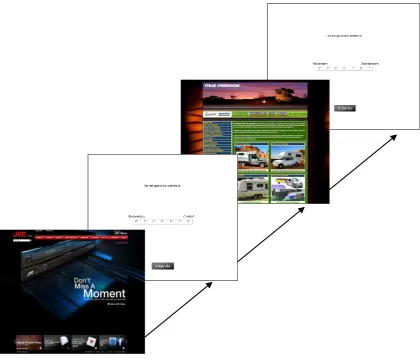
6.7 Screenshots of the experiment

Introduction screen in both conditions

(96)

(97)

Practice phase in both conditions

(98)

Stimuli screenshot websites

(99)

(100)

6.8 Websites used

6.8.1 Fluent websites (low VC – high PT)

Stimuli Name VC_mean VC_sd PT_mean PT_sd Website url

honda 2,708333 2,053188 4,833333 1,761093 http://powersports.honda.com

allete 3,208333 1,718927 4,875 1,701981 http://www.allete.com

pg&e 3,428571 1,68533 5 1,608799 http://www.pge.com

behr 3,777778 2,025479 5,111111 1,502135 http://www.behr.com/Behr/home

harley_davidson 3,772727 1,925563 5,590909 1,469016 http://www.harley-davidson.com

chevrolet 3,590909 1,816829 5,227273 1,631004 http://www.chevrolet.com/#cruze

hebei_yanuo 3 1,752549 5,275862 1,250616 http://www.yanuo.com

sabic 3,454545 1,818615 4,863636 1,753784 http://www.sabic.com/corporate/en

quintiles 3,62963 1,690429 5,407407 1,474378 http://www.quintiles.com

ameresco 3,272727 1,804276 5,454545 1,438494 http://www.ameresco.com

pioneer 3,727273 1,723281 4,636364 1,890967 http://www.pioneerelectronics.com

aiam 2,857143 1,292412 4,928571 1,59153 http://www.globalautomakers.org

northeast_system 3,590909 2,130484 5,136364 1,859223 http://www.nu.com

novasyn_organics 2,928571 1,439246 5,357143 1,499084 http://www.novasynorganics.com

fantasy_junction 2,685714 1,811263 4,828571 1,67131 http://www.fantasyjunction.com

ansa 3,885714 1,761874 5,028571 1,524037 http://ansaautomotive.com

mafs 3,037037 1,580688 5,148148 1,406132 http://www.usemafs.com

engro_corp 3,566667 1,735697 5,233333 1,356551 http://engro.com

national_heat 3,727273 1,723281 4,545455 1,738288 http://www.nationalheatexchange.com

sherwin_williams 3,409091 1,918806 5,136364 1,726418 http://www.sherwin-williams.com

exchange_consulta 2,666667 1,464557 4,25 1,799758 http://www.exchangeconsulting.com

tesla 3,028571 1,932473 5,514286 1,268891 http://www.teslamotors.com

jvc 3,272727 2,229282 5,545455 1,534594 http://www.jvc.com

(101)

6.8.2 Disfluent websites (high VC – low PT)

Stimuli name VC_mean VC_sd PT_mean PT_sd Website url

powermadd 4,214286 1,847184 3,214286 1,368805 http://www.powermadd.com

chase 4,942857 1,679336 3,628571 1,516298 http://www.chase.com

plows_unlimited 4,409091 1,816829 2,772727 1,47783 http://www.plowsunlimited.com/archive

Lloyd 5,142857 1,09945 3,5 1,286019 http://www.lloydsstsb-offshore.com

Taxproblem 4,971429 1,790263 4,057143 1,589355 http://www.taxproblem.org

airgas 4,727273 1,351606 4,318182 1,358794 http://www.airgas.com

chain 4,888889 2,100061 3,185185 1,35978 http://www.chain-auto-tools.com

snl_financial 5,074074 1,356634 4,185185 1,468569 http://www.snl.com

american_express 5,137931 1,186957 4,413793 1,63701 http://www.americanexpress.com

synchem 4,371429 1,800093 3 1,57181 http://www.synchem.com

abraxas 4,541667 2,08471 2,291667 1,517411 http://www.abraxasenergy.com

bank_of_america 5,136364 1,320009 3,818182 1,562549 http://www.bankofamerica.com

geico 5,533333 1,547709 3,6 1,940494 http://www.geico.com

izmocars 4,714286 1,724758 4,228571 1,646488 http://www.izmocars.com

freedom 5,083333 1,529895 3,25 1,823756 http://www.freedomoffroad.com.au

ebizautos 4,851852 1,292097 4,074074 1,858989 http://www.ebizautos.com

horschel 4,733333 1,595972 3,833333 1,821014 http://www.hbpllc.com

first_european 4,818182 1,468279 4 1,573592 http://www.first-european.co.uk

sensient 4,958333 1,680558 3,375 1,68916 http://www.sensient-tech.com

Honeywell 5,296296 1,234592 4,481481 1,451004 http://honeywell.com/Pages/Home.aspx

snowcare_for_troops 4,857143 1,561909 4 1,88108 http://projectevergreen.com/scft

bajaj 4,222222 1,281025 2,925926 1,591466 http://www.bajajauto.com

bureau_van_dijk 5,045455 1,174218 4,045455 1,214095 http://www.bvdinfo.com

(102)

(103)

The fluency effect as the underlying variable for judging beauty and usability

UNIVERSITY OF TWENTE