Monotonicity in Markov chains

(1)

Monotonicity in Markov Chains

Jip Spel

s0

s1

s2

s

3

s

4

p

1

−

p

q

1

−

q

1

−

q

1

−

q

1

−

q

Formal Methods and Tools

Faculty of Electrical Engineering, Mathematics and Computer Science University of Twente

In cooperation with:

(2)

Supervisors:

Prof. Dr. Ir. Joost-Pieter Katoen Prof. Dr. Marielle Stoelinga Sebastian Junges M.Sc.

Location:

Enschede & Aachen

Time Frame:

November 2017– May 2018

(3)

If you weren’t you, then we’d all be

a bit less we

— Piglet, Winnie the Pooh

(4)

Abstract

Markov chains (MCs) are an excellent formalism to capture the behaviour of systems that are governed by randomized behaviour. They are used in computer science, engineering, mathematics, and biology. MCs require fixed distributions, but often these probabilities are not precisely known.

Parametric MCs (pMCs) allow for changing specific sets of distributions in the MC. One way to find the values for parameters is parameter synthesis. Based on the pMC and the specification, the parameter values for which the system meets these requirements are needed to be calculated. We investigate the effect of changing the parameter values. In particular, we observe that parameters often have a monotone effect on the probability that a given system state is reached.

We want to exploit this monotone effect to improve the analysis on the behaviour of systems. To that end, we provide a formal framework to verify efficiently whether these systems are monotone. The framework consists of two layers: the foundation, and the top layer. In the foundation we define a set of monotone pMCs through the composition of predefined building blocks. In the top layer, we show that structures in high level descriptions of systems naturally map to the building blocks of the foundation.

(5)

If you don’t know anything about computers, just remember that they are machines that do exactly what you tell them but often surprise you in the result

— Richard Dawkins [1]

Acknowledgements

I would first like to thank my supervisors Sebastian, Joost-Pieter and Marielle for their time reading (and re-reading) my earlier versions of this master’s thesis. Especially I thank Sebastian, the door to his office was always open whenever I had a question about my research or writing.

Next, I thank everyone at the Chair for Software Modeling and Verification at RWTH Aachen University for their support and all the social events, in particular the hours we spent playing kicker.

I would also like to acknowledge Sybe and Meike for their time to proof-read this thesis and their advice.

Finally, I must express my gratitude to my family, my boyfriend, Leonie, study friends, and Skeuvel for their support through the process of researching and writing this thesis. This accomplishment would not have been possible without you.

(6)

Part II

Framework: Foundation

5 Mapping process algebra to pMC 26 5.1 Process algebra . . . 26

5.2 From process to pMC . . . 28

5.3 Building Blocks . . . 30

5.3.1 Cycles . . . 31

(7)

CONTENTS vii

6 Monotonicity in pMCs 33

6.1 Acyclic composition . . . 34

6.1.1 General Composition . . . 34

6.1.2 Composition of building blocks with the same function . . 37

6.1.3 Composition of building blocks with different functions . 42 6.2 Cyclic composition . . . 44

6.3 Monotonicity and turning points . . . 45

Part III

Framework: Application

7 MappingpWhile to process algebra 48 7.1 Restrictions onpWhile . . . 49

7.2 Probabilistic While language and PA . . . 49

7.2.1 Reducing the process of a program . . . 52

7.2.2 Examples on loops . . . 54

7.3 Equivalence probabilistic choice and if statement . . . 57

8 Monotonic pWhileprograms 59 8.1 General Considerations . . . 61

8.2 Boolean expressions . . . 65

8.3 Program statements . . . 68

8.3.1 Empty statement and variable assignment . . . 68

8.3.2 Probabilistic choice and if statement . . . 69

8.3.3 While loops . . . 70

8.3.4 Sequential composition . . . 73

9 Case Studies 76 9.1 BRP . . . 76

9.2 Zeroconf . . . 83

9.3 Load-unload . . . 84

9.4 Grids . . . 86

9.4.1 Reach a goal in at mostk steps . . . 86

9.4.2 Probability of reaching good before reaching bad . . . 88

9.5 Crowds . . . 90

9.5.1 Using Theory of Chapter 8 . . . 90

9.5.2 Using Theory of Chapter 6 . . . 91

9.5.3 Adaptation of crowds . . . 93

(8)

Part IV

10 Conclusion 96

10.1 Summary . . . 96

10.2 Future work . . . 97

Bibliography 98 Appendix: Proof of Lemma 6.9 101

List of Tables

5.1 Structural operational semantics of PA . . . 29

5.2 Process terms for the building blocks of Figure 5.2 . . . 31

6.1 Monotonicity ofsolM givenf↑p . . . 38

9.1 Results for the case studies . . . 77

9.2 Values of the program variables at different states . . . 92

(9)

List of Figures

1.1 DTMCDof tossing two different biased coins . . . 3

1.2 pMCMof tossing two different parametric coins . . . 4

2.1 Example of a DTMCD . . . 7

2.2 Example of a pMC and an induced pMC . . . 8

2.3 Example of a MDP and MC of this MDP induced by a schedulerσ 10 2.4 Regionrof intervalsI(p) = [0.3,0.7] andI(q) = [0.2,0.4] . . . 11

2.5 Example on relaxation and substitution . . . 12

2.6 Critical points of univariate functions . . . 14

2.7 Multivariate functions . . . 15

4.1 Regionrof intervalsI(p) = [0.3,0.7] andI(q) = [0.2,0.4] . . . 22

4.2 pMCDmonotone in p . . . 23

4.3 Subsets on pMCs . . . 23

4.4 Structures of the While language . . . 24

5.1 pMCMfor processPin Listing 5.1 . . . 29

5.2 The building blocks for constructing pMCs . . . 30

5.3 pMCMfor the process termuf ? l1f : b1f . . . 31

5.4 Cycles in pMCs . . . 32

6.1 pMCM=uf?ug:uh . . . 36

6.2 pMCM=uf?(lif? )m: (bif : )n . . . 41

6.3 pMCM=uf ? l1g : b1h. . . 44

9.1 pMC of brp forN = 2 andMAX= 2 . . . 79

9.2 pMC of Zeroconf withMAX= 2 . . . 84

9.3 Part of the pMC of Crowds [2] . . . 92

9.4 Part of the pMC of Crowds [3] . . . 93

(10)

Listings

2.1 The While language . . . 16

2.2 Example of a programProg. . . 17

5.1 Example of a processP . . . 28

5.2 Process terms for g uf . . . 32

5.3 Process terms for g uf . . . 32

7.1 Example of apWhileprogramProg . . . 51

7.2 ProcessPof programProgin Listing 7.1 . . . 51

7.3 ProgramProgobtained from program statementSand Boolean expressionb. . . 52

7.4 Process terms ofPin Listing 7.2 after steps replace and remove . 53 7.5 ProcessPredof processPin Listing 7.2 . . . 54

7.6 Program of which the process is equivalent to process g P(S). 55 7.7 Process of thepWhileprogram of g uf . . . 56

7.8 Program of which the process is equivalent to process g P(S). 57 7.9 Probabilistic choice with Pr η_post|=_Jstate=1_K=f . . . 57

7.10 If then else with Pr η_post|=_Jstate=1_K=f . . . 58

8.1 While loop . . . 70

8.2 Example of a while loop . . . 71

9.1 ProgBRP, BRP in pWhile . . . 79

9.2 Zeroconf inpWhile . . . 83

9.3 Load and unload in at most k steps . . . 85

9.4 Grid in which the goal is to reach a given state in at most k steps. 87 9.5 Grid in which the goal is to reach a good state before a bad state. 89 9.6 Crowds [3] inpWhile . . . 91

9.7 Crowds [3] inpWhileafter looking at the associated pMC . . . 93

(11)

Acronyms and Notation

DTMC discrete-time Markov chain MC Markov chain

MDP Markov decision process PA Process algebra

pMC parametric Markov chain pWhile Probabilistic While language ↑p Monotone increasing inp

↑ Monotone increasing in any parameter ↓p Monotone decreasing inp

↓ Monotone decreasing in any parameter

7p Not monotone inp

7 Not monotone in any parameter ?p Do not know if monotone inp

? Do not know if monotone in any parameter

(12)

(13)

Part I

Background

(14)

Chapter 1

Introduction

Probabilistic behaviour occurs in several kinds of systems. For instance systems containing randomized algorithms and communication protocols have proba-bilistic state changes. Moreover, the unreliable or unpredictable behaviour in computer networks is viewed as probabilistic behaviour. The occurrence of probabilistic behaviour has led to research on formal methods for the speci-fication and verispeci-fication of probabilistic systems. For instance, the bounded re-transmission protocol [4] (BRP) could be analyzed through formal methods. BRP is meant to transfer a file in a reliable manner, properties such as “the probability that the file is transferred correctly if messages are lost with a prob-ability 0.05” could be analyzed through formal methods.

Markov chains (MCs) are often used to describe probabilistic models. If all transitions between states are probabilistic, the system can be modeled with discrete-time Markov chains (DTMCs).

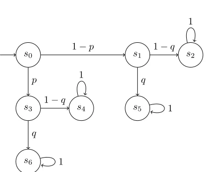
Example 1.1

We consider someone tossing two biased coins. Let the first coin toss head with probability 1₄and the second coin toss head with probability 1₃. Figure 1.1 shows the associated DTMC, in which the person first tosses the first biased coin, and then tosses the second biased coin. At state s2, tails is thrown twice, at state

s4 and s5 heads is thrown once and tails is thrown once. At states6, heads is

thrown twice. ∗

Parametric MCs (pMCs) are used when probabilities of a probabilistic model aren’t known in advance, they generalize DTMCs by allowing parametric prob-abilities instead of fixed probprob-abilities. E.g. in biochemical reaction networks [5] in which the rates of the reactions are either unknown or estimated with a possible measurement error. In these biochemical reaction networks, one still wants to show the robustness of the chemical network.

(15)

(16)

(17)

Introduction 5

naturally to the building blocks in the foundation.

In the foundation, we show how to obtain monotonicity from the structure of pMCs. To this end, we provide the following:

A mapping from a process in PA to a pMC. Theorems on monotonicity in pMCs.

The theorems in the foundation are proven by function calculus.

In the top layer, we show how the results of the foundation are used to obtain monotonicity from the structure of apWhileprogram. We show the following results:

A mapping from apWhileprogram to a process in PA. Theorems on monotone structures inpWhile.

The theorems are proven using the mapping frompWhileprogram to a process, the mapping from a process to a pMC, and the theorems in the foundation. We rewrite several case studies to be in pWhile and show how the obtained results are used to deduce monotonicity for these case studies.

1.3

Structure

(18)

Chapter 2

Preliminaries

In this section we introduce the definitions and notations on Markov chains and Markov decision processes. Secondly, we introduce the theory of parameter lift-ing. Thirdly, we introduce some notations on rational functions and monotone functions. Finally, we introducepWhilein which the case studies are written.

2.1

Markov Chains

A discrete-time Markov chain (DTMC) is a transition system in which tran-sitions to successor states depend on probabilistic choices. Furthermore, the probability of moving from one state to another, only depends on the current state. This is known as the memoryless property. We describe DTMCs as a directed graph where the nodes of the graph are the different states. The tran-sitions are described by a probability matrix and states are labelled with the atomic propositions which hold in that state.

Definition 2.1.1 (Discrete-time Markov Chain [9])

A discrete-time Markov Chain (DTMC) is a tupleD= (S, s0,P, AP, L) where

S is a finite set ofstates

s0∈S is theinitial state

P:S×S7→[0,1] is aprobability matrix such that for alls∈S: P

t∈SP(s, t) = 1

AP is a set ofatomic propositions

L:S 7→2AP _{is a}_{labelling function} _{which gives the atomic propositions that}

hold in a state. ∗

(19)

(20)

(21)

Preliminaries 9

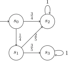
Example 2.4

Recall pMCDfrom Figure 2.2a on the preceding page. ForDvaluation u:{p→ 1

5, q→ 1

3}, is a well-defined and graph preserving valuation. Figure 2.2b

shows the MC induced byu. ∗

2.2

Markov Decision Process

A Markov decision process (MDP) is a transition system in which transitions to successor states are non-deterministic choices over probability distributions over states, so it can be viewed as a MC extended with non-deterministic transitions. Definition 2.2.1 (Markov decision process [11])

AMarkov decision process (MDP) is a tupleM= (S, s0,P, AP, L, Act) where

S,s0,AP andLare defined as in Definition 2.1.1

Actis a finite set of actions

P: S×Act×S 7→ _Q∩[0,1] where for all states s ∈ S and actions α ∈ Act: P

s0_∈_SP(s, α, s0) ∈ {0,1} andAct(s) 6=∅. (Act(s) = {α∈ Act|∃s0 ∈

S.P(s, α, s0)6= 0}) ∗

An action αisenabled in states∈S when∃s0∈S.P(s, α, s0)6= 0.

To reason about the probabilities in a MDP, we need a way to handle the non-determinism. Therefore, schedulers are introduced, a scheduler chooses in each states∈S an enabled action α∈Act(s), which is performed.

Definition 2.2.2 (Scheduler)

A scheduler for MDP M = (S, s0,P, L, Act) is a functionσ : S → Act with

σ(s)∈Act(s) for all s∈S. ∗

Imposing a scheduler σon a MDPMresolves the non-determinism in Mand yields MCMσ, in which the transition probabilities for a state sinMσ equal

those of taking actionσ(s) in statesinM.

Definition 2.2.3 (MC of an MDP induced by a scheduler [6])

Let M = (S, s0,P, AP, L, Act) a MDP and σ a scheduler for M. Markov

chain Mσ induced by applying scheduler σ on MDP M is given by Mσ =

(S, s0,Pσ, AP, L, Act) with

Pσ(s, s0) =P(s, σ(s), s0) for alls, s0∈S ∗

Example 2.5

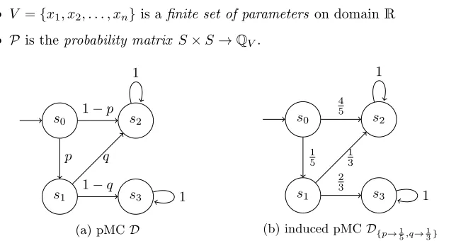
Figure 2.3a on the following page shows a MDPMin which at both states0and

s1a deterministic choice occurs. One can either take the dashed or the

(22)

(23)

Preliminaries 11

r

p q

0 0.3 0.7 1

0 0.2 0.4 1

Figure 2.4: Regionrof intervalsI(p) = [0.3,0.7] andI(q) = [0.2,0.4]

ondly, the parameter transitions aresubstituted by non-deterministic choices on the upper bound and lower bound of the valuations of the parameters in the region. This results in a MDP on which different schedulers are used to obtain the maximal and minimal reachability probabilities. With these reachability probabilities we claim that a region is either safe, unsafe or unknown.

Definition 2.3.2 (Relaxation [11])

Therelaxation of pMCD= (S, s0,P, AP, L, V) is the pMC

rel(D) = (S, s0,P0, AP, L, relD(V)) with: relD(V) ={xis|xi∈V, s∈S}

P0_{(s, s}0_{) =}_P_{(s, s}0_)[x

1, . . . , xn/xs1, . . . , xsn] ∗ Definition 2.3.3 (Substitution)

An MDP subr(M) = (S, s0,Psub, AP, L, Actsub) is the parameter-substitution

of a pMC M= (S, s0,P, AP, L, V) and a region rwhen:

Actsub=

[

s∈S

{v:Vs→R|v(xi)∈B(xi)}

Psub(s, v, s0) =

(

P(s, s0)[v] if v∈Actsub(s),

0 otherwise. ∗

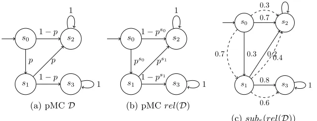
Example 2.7

Figure 2.5a on the following page shows a pMC D with param p used both on the transitions from s0 and the transitions from s1. Figure 2.5b shows the

relaxed pMC rel(D) in which parameter pis split in two seperate parameters ps0 _and_ps1_{. Figure 2.5c shows the parameter-substitution of}_rel(_D_{) with region}

(24)

(25)

Preliminaries 13

Definition 2.4.3 (Multivariate monotone function) Letf :_Rn _→

R.

f ismonotone in parameter xi∈Rwhen eitherf↑xi or↓xi

f ismonotone when eitherf↑ orf↓ ∗

From function theory we know that: f↑xi ↔ ∀~x∈R

n_. ∂

∂xif(~x)≥0

f↑ ↔ ∀i∈[1. . . n].f↑xi

Critical Points and Turning Points

Thecritical points of univariate functionf are the values within its the domain in which the derivative of f is 0. These points can either be turning points or

inflection points. Alocal extreme value always occurs at a turning point. This is tested with the second derivative test.

Remark. The second derivative test is inconclusive when the second derivative is 0, in these cases a higher derivative test can be used.

Definition 2.4.4 (Critical points univariate function) Letf :_R→_Rbe continuous.

v∈_Ris acritical point forf ↔f0(v) = 0 ∗

Definition 2.4.5 (Second derivative test)

Given twice differentiable functionf with critical pointv. Then: f00(v)<0 =⇒f has a local maximum atv f00(v)>0 =⇒f has a local minimum atv

f00(v) = 0 =⇒ the test forf is inconclusive ∗

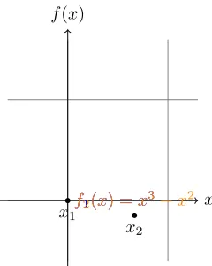
Example 2.8

Figure 2.6 shows the critical points of functions f1 and f2. f1 has a critical

point atx1. The second derivative test is forf1 however, inconclusive. f2has a

critical point atx2as well, forf2the second derivative test shows us thatf2has

a local maximum at x1. The second derivative test forf2 atx2is inconclusive

at this point. ∗

(26)

14 2.4. Functions

x f(x)

f1(x) =x3

f2(x) =x3−x2 x1

x2

Figure 2.6: Critical points of univariate functions

Definition 2.4.6 (Critical points multivariate function) Letf :_Rn→_Rbe continuous.

~v∈_Rn _{is a}_{critical point} _for_f _in_v

i⇐⇒fvi

0_(~_{v) = 0} ~

v∈_Rn is a critical point forf ⇐⇒ ∀i∈[1. . . n].fvi

0

(~v) = 0 ∗

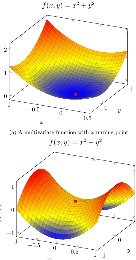
Definition 2.4.7 (Second derivative test multivariate)

Suppose that the second partial derivatives off :_Rn→_Rare continuous on a ball with center~x, with~xa critical point off.

TheHessian matrix is the square matrix of the second-order partial derivatives. For Hessian matrixhindex (i, j) is given byhi,j=

∂2_f

∂xi∂xj

.

Let h denote the Hessian matrix of second partial derivatives and for each k= 1,2, . . . , nletDk denote the determinant of the Hessian in the parameters

x1, x2, . . . , xk. Assume that|H(~x)| 6= 0.

IfDk(c)>0 for allk= 1,2, . . . , nthenf has a local minimum at c~x

if (−1)Dk(c)>0 for allk= 1,2, . . . , n thenf has a local maximum at~x

otherwisef has a saddle point at~x ∗

A saddle point is a critical point of a multivariate function which is not an extremum.

Example 2.9

(27)

Preliminaries 15

−1

−0.5

0

0.5 0

1 0

1 2

x

y

f

(

x, y

) =

x

2

+

y

2

(a) A multivariate function with a turning point

−1

−0.5 ₀

0.5 ₁ −1

0 1 −1

0 1

x

y

f

(

x,

y

)

f

(

x, y

) =

x

2

−

y

2

(b) A multivariate function with a saddle point

(28)

16 2.5. While Language

Monotonicity and turning points

For a univariate functionf we know that givenvis a local maximum,f↑closely to v and f↓ from v until another turning point or boundaries of the interval. Whenvis a local minimum, it holds vice versa.

Definition 2.4.8 (Monotonicity around a local maximum of an univariate function)

Let f : _R → _R with turning point v ∈ _R and points v1, v2 ∈ R such that

v1< v < v2 andf is monotone on (v1, v] and [v, v2).

v is a local maximum ↔f ↑ on (v1, v] andf ↓ on [v, v2) ∗

For a multivariate function f we know that if~v is a local maximum, f↑ to~v andf↓from~vuntil another turning point or boundary of the interval. When~v is a local minimum, it holds vice versa.

Definition 2.4.9 (Monotonicity around a local maximum of a multivariate function)

Let f :_Rn _→

R with turning point~v ∈ _Rn _{and points} _v_~

1, ~v2 ∈Rn such that

~

v1 < ~v < ~v2 for all variables in~v, v~1 andv~2 and f is monotone on (v~1, ~v] and

[~v, ~v2).

~v is a local maximum ↔f ↑ on (v~1, ~v] andf ↓ on [~v, ~v2) ∗

Remark. When a multivariate functionf has a critical point for parametervi,

and this critical point is independent of the values of the other parameters, the theory on the univariate functions is applicable.

2.5

While Language

The While language is a simple programming language, used in the theoretical analysis of imperative programming language semantics. The While language consists of arithmetic expressions, Boolean expressions and program statements. Listing 2.1 gives the abstract syntax of the While language. In this listing,ais an arithmetic expression,nis a natural number,bis a Boolean expression, and S is the program statement.

a ::= n | x | a1 + a2 | a1 * a2 | a1 - a2

b ::= true | false | a1 = a2 | a1 ≤ a2 | ¬b | b1 ∧ b2

S ::= x : =a | skip | S1;S2 | if b then S1 else S2 |

while b do S

Listing 2.1: The While language

(29)

Preliminaries 17

Definition 2.5.1 (Program in pWhile)

The syntax of a programProgwritten inpWhileis denoted by: a ::= n | x | a1 + a2 | a1 * a2 | a1 - a2

b ::= true | false | a1 = a2 | a1 ≤ a2 | ¬b | b1 ∧ b2

S ::= x := a | skip | S1;S2 | if b then S1 else S2 |

while b do S | S1 [f] S2

Prog ::= S; return;

where

ais anarithmetic expression

nis defined on a bounded integer interval (_Zbound)

bis aBoolean expression

Sis aprogram statement

x∈V arProg withV arProgthe set of program variables ofProg

f ∈QV is a rational functions over the set of parametersV

Progis the program. ∗

Example 2.10

Listing 2.2 shows a program Prog in which a biased coin is flipped. With probability p, state will be set to 0 and the program will terminate. With probability 1−p, the program will setstateto1and the while loop is entered. The while loop is executed at most three times. ∗

state := 0 [p] state := 1; count := 1;

while count <= 3 ∧ state = 1 do

state := 0 [p] state := 1; count := count + 1;

return;

Listing 2.2: Example of a program Prog

Boolean variable assignment We writex := binstead of if b then

x := 1;

else

x := 0;

(30)

18 2.5. While Language

Booleans InpWhileonly{=,<=,¬and∧}are defined. Clearly, {<, >=,>,6= and∨} are syntactic sugar for combinations of

{=, <=,¬and∧}. In the remainder of this thesis we use inpWhileprograms both{=,<=,¬and∧}and{<,>=,>,6= and∨}.

(31)

Chapter 3

Related Work

In this chapter we discuss the work related to parameter synthesis and different tools developed for probabilistic model checking.

3.1

Parameter Synthesis

Daws [9] proposes a language-theoretical approach to determine the parametric reachability probability of DTMCs. First of all, Daws converts the parametric DTMC to a FSA. Secondly, a regular expression is computed with the help of state elimination. This expression is then evaluated into a closed-form function representing the reachability property. All parameters must be strictly positive since a transition between two states is only present in the derived FSA when it corresponds to a strictly positive probability.

Hahn et al. [10] investigate how Daws’s idea can be turned into an efficient procedure. The bottleneck in Daws’s idea is the growth of the regular expression relative to the number of states. To overcome this problem Hahn et al. intertwine the regular expression computation with its evaluation. In this way an efficient method is created which avoids a blow up in most practical cases. Although in the worst case the size of the final rational function is stillnO(logn), withnthe number of states.

Quatmann et al. [11] introduce parameter lifting, which is described in Sec-tion 2.3.

Barnat et al. [12] apply LTL model checking procedures directly on a graph representing the dynamics of all possible valuations of parameters. Barnat et al. make use of parameterized Kripke structures to describe the models. The most significant difference between Barnat et al. [12] and the work described before is that the number of valuations of parameters in a parametric Kripke structure

(32)

20 3.2. Tools for probabilistic model checking

is finite, whereas with the pMCs, the parameters can have any well-defined valuation in_R.

3.2

Tools for probabilistic model checking

There are several tools developed for probabilistic model checking. IscasMc [13] allows model checking on MCs and MDPs with LTL, PCTL and PCTL* specifications. MRMC [14] supports PCTL and CSL model checking. LTSmin [15] has developed into a model checker with multi-core algorithms for on-the-fly LTL checking with partial-order reduction, and multi-core symbolic checking for the modalµ-calculus, based on the multi-core decision diagram package Sylvan. Through SCOOP [16], probabilistic models can be checked with LTSmin. Storm [17] can model check both discrete- and continuous-time MCs and MDPs. Prob-lem with these tools, and several other model checking tools, is that they don’t allow for parametric model checking. HyTech analyses linear hybrid automa-ton [18] which is a mathematical model for dynamical systems whose behaviour exhibit both discrete and continuous changes. The tool can perform parameter analysis for linear hybrid automaton with temporal logic requirements. Since pMCs also contain non-linear functions, HyTech isn’t useful to further investi-gate.

(33)

Chapter 4

Problem Description and

Approach

In this chapter, we describe a set of problems which can be solved by formal methods. Then, we elaborate on our approach in this research.

4.1

Problem Description

We considerreachability probabilities on MCs. Let PrD_s(_♦T) denote the proba-bility of eventually reaching a statet∈T ⊆S starting from a states∈S, given DTMCD. PrD(_♦T) refers to this probability starting from initial states0.

Letϕreach =P≥λ(♦T) denote thereachability propertyasserting that eventually

a state inTis reached with at least probabilityλ∈(0,1). We denoteD |=ϕreach

if and only if PrD(_♦T)≥λ.

4.1.1 Formalisation of the problems

Given a pMC D= (S, s0,P, AP, L, V), set of target states T ⊆S and

reacha-bility propertyϕreach. Let SAT be{u|uis graph-preserving andDu|=ϕreach}.

In Problems 3 and 4 we assume SAT 6=∅. We define the problems as follows: 1. SAT =∅

2. Check if regionr⊆SAT 3. Find anyu∈SAT

4. Findu∈SAT such that PrDu₍

♦T) =maxu0_∈_SATPrDu0(♦T)

(34)

22 4.1. Problem Description

4.1.2 Observations

Given a pMC D = (S, s0,P, AP, L, V) with reachability probability PrD(♦T)

we first of all observe that when PrD(_♦T) is monotone in avi∈V, solving the

problems might become easier.

AssumeV={p, q}withp, q∈[0,1]. Given that PrD(_♦T) is monotone increasing inp. Then the problems described above can be simplified by:

1. SAT =∅

To show SAT = ∅, it is sufficient to show that ∀q ∈ [0,1] and p = 1 PrD(_♦T) = 0.

2. Check if regionr⊆SAT

Let region r consist of intervals I(p) = [0.3,0.7] and I(q) = [0.2,0.4], this region is shown in Figure 4.1. Given the monotonicity in p, it is sufficient to show that all points on the line from (0.3,0.2) to (0.3,1.6), described by p= 0.3 and q∈[0.2,0.4], are in SAT. These are all the points on the thick line in Figure 4.1.

3. Find anyu∈SAT

When it is known that PrD(_♦T) is monotone increasing in p, we takepas high as possible inu. When we know SAT6=∅, there will be anu∈SAT, with this highest value of p. So we are left finding a value for qin u, such that u∈SAT.

4. Findu∈SAT such that PrDu₍_♦_T_{) =}_max

u0_∈_SAT

When it is known that PrD(_♦T) is monotone increasing in p, we takepas high as possible in u. So we are left with finding the value ofq in u, such that PrDu₍

♦T) =maxu0_∈_SAT.

r

p q

0 0.3 0.7 1

0 0.2 0.4 1

(35)

Problem Description and Approach 23

s0 s1 s2

s3 s4

p

1−p

1

q

1−q

q

1−q

q

1−q q

1−q

1

Figure 4.2: pMCDmonotone in p

Example 4.1

Figure 4.2 shows a pMC, withT ={ }. PrD(_♦T) is monotone increasing inp. Consider Problem 2, a possible region to consider while using parameter lifting is build of I(p) = [0.3,0.7] and I(q) = [0.2,0.4]. Exploiting the monotonicity in p, we only need to look at the lower bound on p, since increasing p will increase the reachability probability. Therefore, we don’t need to split inpwith

parameter lifting. ∗

Secondly, we observe for small pMCs it is easy to determine if Pr≥λ(♦T) is

monotone in parameters ofV (the clearly monotone pMCs in Figure 4.3). We can obtain the rational function and check, with basic function theory, if the rational function is monotone. However, this is not possible for larger pMCs, since the rational functions get too large.

(1) pMCs

(2) Monotone pMCs

(3) Clearly

monotone pMCs

(36)

24 4.2. Approach

Our hypothesis is that pMCs which are known to be monotone in parameters ofV can be constructed from simple, clearly monotone, pMCs. So we can find a subset of (2) in Figure 4.3, that includes (3). However, it may be hard to find this construction. The risk is that it can be complicated in either time or space.

4.1.3 Problem statement

We want to find monotonicity in pMCs without analyzing the whole rational function and apply this on structures in high level descriptions.

4.2

Approach

We provide a framework to deduce monotonicity of MCs. We describe in a compositional way, a subset of pMCs which are guaranteed to be monotone in one or more parameters. We provide proofs of the monotonicity of this subset of pMCs. As it might be hard to find a way to compose larger monotone pMCs from the small pMCs. We describe structures inpWhile, which map to a subset of pMCs which are monotone. We then show how we transform case studies which are monotone in one or more parameters into the monotone structures of

pWhile.

Less expressive More expressive

y x

Figure 4.4: Structures of the While language

Example 4.2

Figure 4.4 shows the difference in expressiveness of different structures of the probabilistic While language. Everything on the left of point y is monotone in one or more parameters. We try to find a pointx, which is expressive enough to use in our case studies and is guaranteed to be monotone in one or more

parameters. ∗

For this research the following questions must be answered.

1. Which subset of pMCs is monotone in one or more parameters?

2. Which structures inpWhilehave an underlying pMC which is monotone in one or more parameters?

3. Can improvement in the run time of parameter lifting be achieved by ex-ploiting the monotonicity?

(37)

Part II

Framework: Foundation

(38)

Chapter 5

Mapping process algebra to

pMC

We use processes in PA to describe both pMCs andpWhileprograms. We make use of processes, as this is a concise way to describe both pMCs and pWhile

programs. Theorems on monotonicity in pMCs (Chapter 6), are defined on the process algebras of the pMCs. By mapping pWhile programs to process algebras (Chapter 7), we obtain theorems on the monotonicity in structures in

pWhile(Chapter 8).

Process algebras are used for modelling and reasoning about the functional aspects of concurrent processes. Jonsson et al. [23] introduce a probabilistic process algebra (PCCS) for Markov decision processes. Our process algebra (PA) is an adaptation to PCCS and yields probabilistic deterministic processes, in which also Boolean expression may occur.

This chapter provides the introduction of the process algebra PA (Section 5.1) and the mapping from PA to pMCs (Section 5.2). Furthermore, it provides the PA notation of different building blocks of pMCs (Section 5.3), these blocks are used in Chapter 6.

Notation. For any function f(p1, . . . , pn), we write f instead. We use this

notation throughout this thesis.

5.1

Process algebra

We give a formal definition of the syntax of a process term in PA (Defini-tion 5.1.1). This allows us to define processes in PA as the pair of an initial process term (Definition 5.1.2) and the set of process terms.

(39)

Mapping process algebra to pMC 27

Definition 5.1.1 (Syntax process term) The syntax of a process term in PA is given by:

Proc ::= | | Pn

i=1fi. Proci | Proc1 ? Proc2 : Proc3

where:

is a goal process term, is a zeroprocess term, Pn

i=1fi.Prociis a probabilistic sum over process terms withn≥1,fi∈QV

andPn

i=1fi = 1, and

Proc1 ? Proc2 : Proc3is the composition of three process terms. ∗ Definition 5.1.2 (Process)

A process in PA is a pairP= (Proc0, {Proc0, . . . ,Procn}) where

Proc0is the initial process term ofP, and

Proci is a process term for 0≤i≤n. ∗

A process term can either be a goal process term ( ), a zero process term ( ), a probabilistic sum of processes (Pn

i=1fi. Proci) or the composition of different

processes through an if then else statement (Proc1?Proc2:Proc3). In

theif then elsestatement, all occurrences of process term inProc1 are

replaced byProc2 and all occurrences of process term inProc1are replaced

byProc3.

When the probabilistic sum consists of two elements, the binary sum, ⊕f is

used. SoProc1 ⊕f Proc2is shorthand forf.Proc1 + (1−f).Proc2. It is

easy to see that everyn-ary sum can be written as the composition of process terms with the binary sum.

Example 5.1

An example processPis denoted in Listing 5.1. The initial process term ofPis

Proc0. The set of process terms ofPconsists of 5 process terms, of which two

goal process terms and one zero process term. From the initial process term, term Proc1 is taken with probability p, and Proc2 is taken with probability

(40)

(41)

(42)

(43)

Mapping process algebra to pMC 31

Building block Process term

uf ⊕f

l1f ⊕f( ⊕f )

l2f ( ⊕f )⊕f

b1f ( ⊕f )⊕f

b2f ⊕f( ⊕f )

Table 5.2: Process terms for the building blocks of Figure 5.2

Example 5.3

Figure 5.3 shows pMCMcomposed fromuf,l1f, andb1f through

Proc1 ? Proc2 : Proc3.

LetProc1 = uf,Proc2 = l1f, andProc3 = b1f. Through the composition,

the states of Proc1 are replaced by Proc3, and the states of Proc1 are

replaced byProc2. ∗

s0 l0

l1 f

1−f

f

1

b0 b1

f

1−f

f

1 1

1

f

1−f

Figure 5.3: pMCMfor the process term uf ? l1f : b1f

5.3.1 Cycles

(44)

32 5.3. Building Blocks

g P: Replace the states of process P with a process in which we go

with probabilitygto and with probability 1−gto the initial process term ofP.

g P: Replace the states of process P with a process in which we go

with probabilitygto and with probability 1−gto the initial process term ofP.

Proc0 = Proc1 ⊕f Proc2

Proc1 = Proc3 ⊕g Proc0

Proc2 =

Proc3 =

Listing 5.2: Process terms for g uf

Proc0 = Proc3 ⊕f Proc1

Proc1 = Proc3 ⊕g Proc0

Proc2 =

Proc3 =

Listing 5.3: Process terms for g uf

Example 5.4

Figure 5.4a shows the pMC M1 of g uf and Figure 5.4b shows the pMC

M2of g uf. Listing 5.2 shows the process terms for g uf and Listing 5.3

shows the process terms for g uf. The processes of g uf and g uf

both have initial process termProc0. ∗

s0 s1

f 1−f

g 1−g

1

(a) pMCM1 for process term g uf

s0

s1

1−f f

g 1−g

1

(b) pMCM2for process term g uf

(45)

Chapter 6

Monotonicity in pMCs

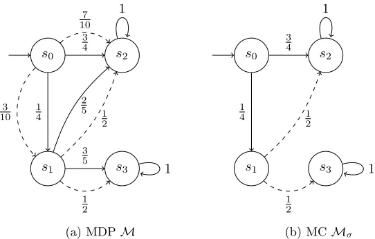
The previous chapter defines a process algebra (PA) for expressing pMCs. In this chapter, we consider monotonicity in the parameters of the probability functions of pMCs. A possible way to find monotonicity in the probability function of eventually reaching a state in a pMC, is to obtain a rational function symbolically expressing the reachability probability and check if this function is monotone for a given parameter. We discuss how monotonicity in pMCs can be obtained from the structure of the pMC without analyzing the rational function. This chapter presents the following results:

For acyclic composition through uf?ug : uh, Theorems 6.3, 6.5, 6.6, 6.8

and 6.11 provide cases in which either monotonicity occurs, or the pMC is not monotone.

For cyclic composition through f2 uf1, Theorems 6.13 and 6.14 provide

cases in which monotonicity occurs.

We start with the acyclic composition of pMCs throughuf?ug:uh(Section 6.1)

and continue with cyclic composition trough f2 uf1 (Section 6.2). In most

theorems we assume f↑p for any graph-preserving valuation and prove that

solM↑p. In a similar manner, theorems for f↓p and claims on solM can be

obtained. In Section 6.3, we show that for some sub-domains of graph-preserving valuations f↑p might hold, and show that the theorems defined in Sections 6.1

and 6.2 can also be applied on these sub-domains.

Notation. LetsolMbe the function describing the probability of reaching state sin pMCMwithL(s) = . Let↑p and↓pbe as defined before,7p denote that

solM is not monotone inpand ?p denote that we do not know whether solM is monotone or not in p. Furthermore, we replace subscript 1 and 2 with i in building blocks b1 and b2 and building blocks l1 and l2 (Section 5.3). We

(46)

34 6.1. Acyclic composition

writef continuous forpi, instead of for: any graph-preserving valuationuwith

u={p0, . . . , pn}, in whichpj is fixed fori6=j,f is continuous.

Assumptions. In the theorems we only consider functionsf for which: ∂

∂pf exists.

Any total valuationu∈Dom(f) is well-defined (Definition 2.1.5).

When we either consider composition with cyclic pMCs, or composition with not monotone structures, we additionally assume all total valuations u∈Dom(f) are graph-preserving (Definition 2.1.6).

We observe that when a parameter p does not occur in function f, f is both monotonically increasing and decreasing inp; Lemma 6.1 formalizes this obser-vation.

Lemma 6.1

Iff is constant in parameterp, thenf↑p andf↓p. ∗ Proof of Lemma 6.1

∂

∂pf = 0 aspdoes not occur inf. Therefore, ∂

∂pf ≥0 and ∂

∂pf ≤0. ∗ Lemma 6.2

Let pMCM=uf, then: f↑p⇐⇒solM↑p ∗ Proof of Lemma 6.2

We obtain the following equalities:

solM=f ∂

∂psolM= ∂ ∂pf

As the derivatives are equal, we obtain _∂p∂ solM≥0 if and only if ∂p∂ f ≥0. ∗

6.1

Acyclic composition

In this section we look at monotonicity of solM in parameter p through the composition of pMCs withM=uf?ug:uh.

6.1.1 General Composition

(47)

Monotonicity in pMCs 35

Theorem 6.3 (General composition) Let pMCMbe described byuf?ug :uh. Then:

1. (f↑p andg≥handg↑p andh↑p) =⇒solM↑p

2. (f↑p andg≤handg↓p andh↓p) =⇒solM↓p ∗

Proof of Theorem 6.3

We provide the proof for Case 1; the proof of Case 2 is obtained in a similar manner. Let solM be the function describing the probability of eventually reaching a state swithL(s) = in pMCM=uf?ug:uh. So:

solM=f·g+ (1−f)·h

By the definition of monotonicity (Definition 2.4.3 on page 13), to obtainsolM↑p

we need to show: _∂p∂ solM≥0. With the product rule we obtain:

∂

∂psolM= ∂ ∂pf·g−

∂ ∂pf·h+

∂ ∂pg·f+

∂

∂ph·(1−f)

By assumption, _∂p∂ f, _∂p∂ gand _∂p∂ hexist. Furthermore,f↑p, so _∂p∂ f ≥0.

To prove ∂

∂psolM≥0, it is sufficient to show that all of the following holds:

∂ ∂pf ·g−

∂

∂pf·h≥0 (6.1)

∂

∂pg·f ≥0 (6.2)

∂

∂ph·(1−f)≥0 (6.3)

We observe the following:

By assumption _∂p∂ f ≥0, sog≥himplies (6.1) holds.

g↑p implies _∂p∂ g≥0. Therefore, (6.2) holds.

h↑p implies _∂p∂ h≥0. Therefore, (6.3) holds.

(48)

Example 6.1

LetM =uf?ug :uh as in Figure 6.1. Assume f =p, g =p+ (1−p)·pand

h = 1₉·p. Take e.g. p ∈ [0,1] then g ≥ h. Furthermore, f↑p, g↑p and h↑p.

Therefore, by Theorem 6.3 Case 1 we obtainsolM↑p. ∗

s0

s2

s1

f

1−f

g

1−g h

1−h

Figure 6.1: pMCM=uf?ug:uh

As sol = 1 and sol = 0, we obtain Corollaries 6.4.a and 6.4.b by combining Lemma 6.1 and Theorem 6.3.

Corollary 6.4

a. Let pMCM=uf?ug: . Then:

f↑pand g↑p=⇒solM↑p

b. Let pMCM=uf? :uh. Then:

f↑p andh↑p=⇒solM↑p ∗

Theorem 6.5 (Not monotone)

Let pMCMbe described byuf?ug:uh. Then:

1. _∂p∂ f = 0 and _∂p∂ g= 0 andh7p =⇒solM7p

2. ∂

∂pf = 0 and ∂

∂ph= 0 andg7p =⇒solM7p

(49)

We provide the proof for Case 1, the proofs of Cases 2 and 3 are obtained in a similar manner. For Case 1, we have the following functions:

solM=f·g+ (1−f)·h ∂

∂psolM= ∂

∂pf·(g−h) + ∂ ∂pg·f+

∂

∂ph·(1−f)

As _∂p∂ f = 0 and _∂p∂ g= 0, we obtain:

∂

∂psolM= 0·(g−h) + 0·f+ ∂

∂ph·(1−f) = ∂

∂ph·(1−f)

As we only consider graph-preserving valuations (1−f) > 0. So, from h₇p,

solM7p follows. ∗

6.1.2 Composition of building blocks with the same function

In this section, we treat composition through uf?ug :uh, in which f,g andh

might not be monotone. Letuf,ug, anduh be one of the building blocks (see

Section 5.3 on page 30), and assume that these building blocks are all build with the same functionf. Theorem 6.6 provides the results for the following pMCs:

uf?ug:uhwithug, uh∈ { , , uf, lif, bif},

lif?ug:uhwithug, uh∈ { , , uf}, and

bif?ug:uhwithug, uh∈ { , , uf}.

Remark. Tables 6.1b and 6.1c show symmetry, this is caused by the symmetry oflif andbif.

Theorem 6.6 (Composition of building blocks)

For any functionf, withf↑p: solMin Table 6.1 is either 0, 1,↑p,↓por?p. ∗

Remark. Theorem 6.6 is an extension to Theorem 6.3 on page 35. In Theo-rem 6.6 we do not require uf,ug anduh to be monotone in all cases, where in

Theorem 6.3 we require this monotonicity. Proof of Theorem 6.6

We provide the proof foruf? :lif in Table 6.1a. All other proofs are obtained

(50)

uh

uf lif bif

ug

1 ↑p ↑p ?p ↑p

↓p 0 ?p ↓p ?p

uf ?p ↑p ↑p ?p ↑p

lif ?p ↑p ↑p ?p ↑p

bif ↓p ?p ?p ↓p ?p

(a)M=uf?ug:uh

uh

uf

ug

1 ?p ?p

?p 0 ?p

uf ↑p ↑p ↑p

(b)M=lif?ug :uh

uh

uf

ug

1 ?p ↑p

?p 0 ↑p

uf ?p ?p ↑p

(c)M=bif?ug :uh

(51)

(52)

Theorem 6.7

Let fmin be the minimal value of f and fmax the maximal value of f. If

fmin ∈ [0,1₃) and fmax ∈ (2₃,1], then all occurrences of ?p in Table 6.1 are

replaced by₇p. ∗

Asf is a probability function,f ∈[0,1]. For allsolM?pin Table 6.1, we obtain

thatsolM has a turning point within [13, 2

3]. This is proven in a similar way as

for Theorem 6.6. So, for any functionf withfmin∈[0,1₃) andfmax∈(2₃,1] we

obtainsolM7p. ∗

Example 6.3

Recall pMC M in Figure 5.3 on page 31, where ug and uh are denoted by

lif and bif, respectively. Although bothsollif7p and solbif7p, we obtain from

Theorem 6.6 (Table 6.1a) that forM=uf?lif :bif:

solM↑p ∗

Notation. Let (lif? )mbe shorthand for (lif? : (lif? :. . .))

| {z }

mtimeslif

in which we nest

lif mtimes, and let (bif : )nbe shorthand for (bif?(bif?. . .: ) : )

| {z }

ntimesbif

in which we

nestbif ntimes. Ifm= 0, then (lif? )m= , and ifn= 0, then (bif : )n= .

Theorem 6.8

LetM=uf?(lif? )m: (bif : )n. For anym, n∈N, it holds that:

f↑p=⇒solM↑p ∗

Example 6.4

Figure 6.2 shows the pMCM=uf?(lif? )m: (bif : )n. Assumef =p, from

Theorem 6.8 it follows thatsolM↑p. ∗

Lemmas 6.9 and 6.10 will be used to prove Theorem 6.8. Lemma 6.9 provides the case form∈Nandn= 0, where Lemma 6.10 provides the case forn∈N andm= 0.

Lemma 6.9

LetM=uf?(lif? )m: . For anym∈N:

(53)

(54)

Proof of Lemma 6.10

The proof is obtained in a similar manner as the proof of Lemma 6.9. ∗ These results now bring us in a position to prove Theorem 6.8.

The reachability probability inMis given by:

solM=f·(1−(f·(1−f))m) + (1−f)·(f·(1−f))n

We need to showsolM↑p, givenf↑p for anym, n∈N. This is done by simulta-neous induction onmandn.

Base case: m=0, n=0

This case maps to uf? : ,solM↑p follows from Theorem 6.3.

Induction

AssumesolM↑pform≤k,n≤l. We need to show that for bothm=k+ 1,

n=l andm=k, n=l+ 1,solM↑p. – m=k+ 1, n=l

Similar to the proof of Lemma 6.9 with induction hypothesis solM↑p

untilm∈[0, k],n∈[0, l].

– m=k, n=l+ 1

Similar to the proof of Lemma 6.10 with induction hypothesis solM↑p

untilm∈[0, k],n∈[0, l].

By induction onmandnwe obtain: f↑p =⇒solM↑p for anym, n∈N. ∗

6.1.3 Composition of building blocks with different functions

In the previous section, we introduced the composition of building blocks with the same functionf. In this section we extend this to the composition of building blocks with different functions; we obtain Proposition 6.11 and Corollaries 6.12.a and 6.12.b.

Remark. The comparison with 1₂ is introduced by the derivatives ofsollig and

solbih, which need to be≥0 to have monotonicity insolM.

Theorem 6.11

Let pMCM=uf?lig:bih, and letf↑p,g↑p andh↑p. If

1. ((g+ (1−g)2₎_≥_h_·₍₁₋_{h), and}

2. _∂p∂ g= 0 org≥1 2, and

3. _∂p∂ h= 0 orh≤1 2

(55)

Proof of Proposition 6.11

LetsolM be the function describing the probability of eventually reaching a state in pMCM=uf?lig:bih. This function is given by:

solM=f·(g+ (1−g)2) + (1−f)·h·(1−h) Its derivative is given by:

∂

∂psolM= ∂

∂pf·((g+ (1−g)

2₎₋_h_·₍₁₋_h))

+ ∂

∂pg·f ·(2g−1)) + ∂

∂ph·(1−f)·(1−2h) We make the following observations:

If ((g+ (1−g)2₎_≥_h_·₍₁₋_{h) then}

∂

∂pf ·((g+ (1−g)

2₎₋_h_·₍₁₋_h))_≥₀

If either ∂

∂pg= 0 org≥ 1 2 then

∂

∂pg·f·(2g−1))≥0

If either _∂p∂ h= 0 orh≤1 2 then

∂

∂ph·(1−f)·(1−2h)≥0

By these observations, we obtain _∂p∂ solM≥0. ∗

Example 6.5

Figure 6.3 shows the pMC forM=uf?l1g:b1h. Assume f =p,g= 1₂·p2+1₂

and h= 1₄·q. By Proposition 6.11, it follows thatsolM↑p. Furthermore, from

Theorem 6.5 we obtainsolM7q, as _∂q∂ f = 0, _∂q∂soll1g = 0 andsolb1h 7q. ∗

(56)

44 6.2. Cyclic composition

Corollary 6.12

a. Let pMCM=uf?lig: ,f↑p andg↑p:

∂

∂pg= 0 org≥ 1

2 =⇒solM↑p

b. Let pMCMbe given byuf? :bih,f↑p andg↑p:

∂

∂ph= 0 orh≤ 1

2 =⇒solM↑p ∗

s0 l0

l1

g

1−g 1−g

g

1

b0 b1

h

1−h

h

1 1

1 f

1−f

Figure 6.3: pMCM=uf ? l1g : b1h

6.2

Cyclic composition

In this section, we consider monotonicity in pMCs through the composition with

g uf. Theorems 6.13 and 6.13 provide claims on the monotonicity for cyclic

uni-variate pMCs. Note that g uf = ( 1−g u1−f))? : . Theorems for g uf can be deduced by combining Theorems 6.6, 6.13 and 6.14.

Example 6.6

Recall pMC M1 of g uf in Figure 5.4a. We observe that if f↑p and g↑p,

thensolM1↑p. Also iff = 1−g andf↑p, thensolM1↑p. From this observation

(57)

Theorem 6.13

LetM= g uf, then:

1. iff↑p andg↑p thensolM↑p

2. ifg= 1−c·f, c∈(0,1] andf ↑p thensolM↑p ∗

Example 6.7

Recall M = g uf from Figure 5.4a. Assume f = p and g = 1−p, from

Theorem 6.13 Case 2, we obtainsolM↑p. ∗

Theorem 6.14

LetM= 1−g ( g uf), then:

1. iff↑p andg↑p andg≤ 1₂ thensolM↑p

2. iff↑p andg↓p andg≥ 1₂ thensolM↑p ∗

Proof of Theorems 6.13 and 6.14

We provide the proof for Theorem 6.13 Case 1, the proofs of Theorem 6.13 Case 2 and Theorem 6.14 are obtained in a similar manner. Let solM denote the probability of reaching in g uf,f↑p andg↑p). We need to showsolM↑p.

solM= ∞ X

i=0

f·g·(f·(1−g))i

=f·g· 1 1−f·(1−g) ∂

∂psolM=

∂ ∂pf·g+

∂

∂pg·(1−f)·f

(1−f(1−g))2

We make the following observations: (1−f(1−g))2_>_{0, and}

if bothf↑p andg↑p, then _∂p∂ f·g+_∂p∂g·(1−f)·f ≥0

By these observations we obtain ∂

∂psolM≥0. ∗

6.3

Monotonicity and turning points

(58)

46 6.3. Monotonicity and turning points

of a function, we obtain sub-domains at which a function is monotone (Defini-tions 2.4.8 and 2.4.9 on page 16). Theorem 6.15 states that for any sub-domain ofp, we can apply the Theorems introduced in this Chapter.

Theorem 6.15

For any subdomain domsub(f)⊆dom(f), we can apply Lemmas 6.1 and 6.2

and Theorems 6.3-6.14. ∗

Example 6.8

Let pMCM=uf?ug:uh withf =pandg= 1 and h= 1−p+p2.

solM= 1−p+ 2p2−p3 A turning point ofhisp=1₂. So ifp≥1

2 thenh↑p. From Theorem 6.3 Case 1

and Theorem 6.15, we obtain:

ifp∈[1

2,1], thensolM↑p ∗

The proofs are similar as those of the associated theorems, however, we now

(59)

Part III

Framework: Application

(60)

Chapter 7

Mapping

pWhile

to process

algebra

In Chapter 5, we introduced the process algebra PA and used this notion to describe pMCs. Recall that we make use of processes, as this is a concise way to describe both pMCs and pWhile programs. The subset of pMCs which are guaranteed to be monotone in some of their parameters is described in Chapter 6. As it might be hard to find a way to compose larger monotone pMCs from the simple pMCs, the aim of this chapter is to find substructures in

pWhile, which map to the subset of pMCs which are monotone. To this end, we mappWhileto process algebras, and obtain theorems on the monotonicity in structures of pWhile(Chapter 8).

This chapter presents the following results:

Restrictions on the pWhile programs, which are needed for the mapping from pWhileprograms to a process in PA.

The mapping from apWhileprogram to a process in PA.

Equivalence of statementsS1 [f] S2andif b then S1 else S2. In this chapter, we describe how the process algebra PA is used to describe certain programs in pWhile. First of all, we introduce two restrictions on

pWhile (Section 5.2). Secondly, we provide a mapping from pWhile pro-grams to processes in PA (Section 7.2). For this mapping, we assume the

pWhile programs to satisfy the restrictions. The mapping is used, together with the Theorems of Chapter 6, to prove the theorems of Chapter 8. Finally, we show equivalence of the probabilistic choice (S1 [f] S2) and the if state-ment (if b then S1 else S2.) in Section 7.3. For this equivalence, we

(61)

MappingpWhileto process algebra 49

require both the probabilistic choice, and the probability that b holds before executing the if statement, to have the same probability functionf.

7.1

Restrictions on

pWhile

To define the mapping from apWhileprogram to a PA process, we define two restrictions on the programs:

1. The keyword state is reserved for a program variable to track whether the program is in a good (state = 1) or bad (state = 0) state. In the associated process the good and bad state are denoted by and , respectively.

2. At the end of a program,stateshould either contain 0 or 1.

We observe that when a programProgdoes not satisfy these restrictions, we can modifyProgto meet them. We need a Boolean expressionbover the program variables, which states whether or not the program is in a state. The value of state will be 1 if bholds, and 0 otherwise. LetProg ::= S; return;, the modified programProg0 is denoted by: S; state := b; return;.

7.2

Probabilistic While language and PA

Recall the syntax of a program written inpWhile, as denoted in Definition 2.5.1 on page 17. In this section, we provide the mapping from pWhile programs and to processes in PA. We observe that every valuation of program variables together with the program statements (which still need to be executed) maps to a process term. This mapping is formalized as follows:

Definition 7.2.1 (Mapping from pWhileto PA)

Given apWhileprogramProgand the variable valuationη. Let the function

Proc:(V arProg→Zbound)×pWhile→PA

for programProgbe defined as follows: Proc(η, return;)=

(

ifη|=Jstate=1K ifη|=_Jstate=0_K Proc(η, x := a; P)=1.Proc(η{x←a}, P)

Proc(η, skip; P)=1.Proc(η, P)

Proc(η, (if b then S1 else S2); P)

= (

1.Proc(η, S1; P) ifη|=JbK

(62)

50 7.2. Probabilistic While language and PA

Proc(η, (while b do S1); P)

= (

1.Proc(η, (S1; while b do S1); P) ifη|=JbK

1.Proc(η, P) otherwise Proc(η, (S1 [f] S2); P)

=Proc(η, S1; P) ⊕f Proc(η, S2; P)

With:

η: V arProg →Zbound∪ {⊥}the valuation function of V arProg,

V arProg the set of program variables occurring inProg, and

⊥the initial value of any variable inV arProg. ∗

Remark. For valuation of the program variables η: V arProg, let ηpre{S} be

the valuation of the program variables after executing program statement S, given current valuationηpre. Furthermore, let for arithmetic expressiona

(Def-inition 2.5.1), η(a) be the value of a after replacing all program variables by their value inη.

In the definition above, we inductively define the mapping from a pWhile

program to a process term. The process of apWhileprogram is formalized as follows:

Definition 7.2.2 (Process of a program)

The processPin PA of programProginpWhileis defined by:

P(Prog) =Proc(V arProg→⊥, Prog) ∗

Example 7.1

Consider thepWhileprogramProgin Listing 7.1. In each iteration of the while loop, a coin is flipped. This coin determines if we enter the while loop again, or we continue the rest of the program. When the while loop is executed an even number of times, the program will terminate with state = 1. Otherwise, it terminates with state = 0. The associated process P can be found in Listing 7.2 on the next page, in which Pi-j denotes the program statements contained by line-numbersitoj.

Remark. Some process terms are not defined for all variable valuations, as it might not be possible to enter a part of the code for this valuation. E.g. in Listing 7.1, the term Proc({1,1}, P4-5; P3-6) is not defined. With variable valuation{state = 1, c = 1}, it is not possible to enter the while

loop. ∗

(63)

1 state := 0;

2 c := 0 [p] c := 1;

3 while c = 0 do

4 c := 0 [p] c := 1;

5 state := ¬ state;

6 return;

Listing 7.1: Example of apWhileprogramProg

Initial process term: Proc({⊥,⊥}, P1-9)

Proc({⊥,⊥}, P1-6) = 1.Proc({0,⊥}, P2-6)

Proc({0,⊥}, P2-9)

= Proc({0,⊥}, c := 0; P3-6)

⊕p Proc({0,⊥}, c := 1; P3-6)

Proc({0,⊥}, c := 0; P3-6) = 1.Proc({0,0}, P3-6)

Proc({0,⊥}, c := 1; P3-6) = 1.Proc({0,1}, P3-6)

Proc({0,0}, P3-6) = 1.Proc({0,0}, P4-5; P3-6) Proc({0,1}, P3-6) = 1.Proc({0,1}, P6)

Proc({1,0}, P3-6) = 1.Proc({1,0}, P4-5; P3-6) Proc({1,1}, P3-6) = 1.Proc({1,1}, P6)

Proc({0,0}, P4-5; P3-6)

= Proc({0,0}, c := 0; P5; P3-6)

⊕p Proc({0,0}, c := 1; P5; P3-6)

Proc({1,0}, P4-5; P3-6)

= Proc({1,0}, c := 0; P5; P3-6)

⊕p Proc({1,0}, c := 1; P5; P3-6)

Proc({0,0}, c := 0; P5; P3-6) = 1.Proc({0,0}, P5; P3-) Proc({0,0}, c := 1; P5; P3-6) = 1.Proc({0,1}, P5; P3-6)

Proc({1,0}, c := 0; P5; P3-6) = 1.Proc({1,0}, P5; P3-6) Proc({1,0}, c := 1; P5; P3-6) = 1.Proc({1,1}, P5; P3-6)

Proc({0,0}, P5; P3-6) = 1.Proc({1,0}, P3-9)

Proc({0,1}, P5; P3-6) = 1.Proc({1,1}, P3-9) Proc({1,0}, P5; P3-6) = 1.Proc({0,0}, P3-9) Proc({1,1}, P5; P3-6) = 1.Proc({0,1}, P3-9)

Proc({0,1}, P9) =

Proc({1,1}, P9) =

(64)

Definition 7.2.3 (Equivalence of programs)

ProgramsProg1 andProg2 are equivalent if and only if their processes

P(Prog1)and P(Prog2)are equivalent (Definition 5.2.2). ∗

So far, we have shown how to obtain the process of a program. When proving theorems for conditions for monotonicity ofpWhileprograms, we need to know the process of a program statement S. Therefore, we need to know the goal, denoted by Boolean expressionb, we want to achieve after executingS. When

b holds after executing Swe set stateto 1. Otherwise, we set state to 0. We formalize this in Definition 7.2.4.

Definition 7.2.4 (Process of a program statement)

The process of program statementS, with Boolean expressionboverS, is given by the process of the programProgin Listing 7.3.

S;

state := ¬b;

return;

Listing 7.3: Program Prog obtained from program statement S and Boolean expressionb.

∗

7.2.1 Reducing the process of a program

Process Pof a pWhile program can often be rewritten to obtain less process terms. A processQthat is equivalent toP, andQhas less process terms thanP

is called areduced process ofP. In this section, we provide an example in which we obtain a reduced processPred.

Example 7.2

ProcessPof Listing 7.2 can be reduced to processPred in Listing 7.5. This can

be done in the following manner:

1. Replace all occurrences ofProc1 = 1.Proc2 andProc2 = Proc3 by

Proc1 = Proc3.

2. Remove all superfluous process terms. 3. Merge similar process terms.

(65)

Proc({⊥,⊥}, P1-9)

= Proc({1,⊥}, c := 0; P3-9)

⊕p Proc({1,⊥}, c := 1; P3-9)

Proc({1,⊥}, c := 0; P3-9)

= Proc({1,0}, c := 0; P5-8; P3-9)

⊕p Proc({1,0}, c := 1; P5-8; P3-9)

Proc({1,⊥}, c := 1; P3-9) =

Proc({0,0}, P3-9)

= Proc({0,0}, c := 0; P5-8; P3-9)

⊕p Proc({0,0}, c := 1; P5-8; P3-9)

Proc({1,0}, P3-9)

= Proc({1,0}, c := 0; P5-8; P3-9)

⊕p Proc({1,0}, c := 1; P5-8; P3-9

Proc({0,0}, c := 0; P5-8; P3-9)

= Proc({1,0}, c := 0; P5-8; P3-9)

⊕p Proc({1,0}, c := 1; P5-8; P3-9

Proc({0,0}, c := 1; P5-8; P3-9) = Proc({1,0}, c := 0; P5-8; P3-9)

= Proc({0,0}, c := 0; P5-8; P3-9)

⊕p Proc({0,0}, c := 1; P5-8; P3-9)

Proc({1,0}, c := 1; P5-8; P3-9) =

(66)

Initial process term: Proc0

Proc0 = Proc1 ⊕p Proc2

Proc1 = Proc0 ⊕p Proc4

Proc2 =

Proc4 =

Listing 7.5: ProcessPred of processPin Listing 7.2

In the first step we can replace inP:

Proc(\{⊥,⊥\}, P1-9) = 1.Proc(\{1,⊥\}, P2-9)

by:

Proc({⊥,⊥}, P1-9)

= Proc({1,⊥}, c := 0; P3-9)

⊕p Proc({1,⊥}, c := 1; P3-9)

By the replacement, Proc({1,⊥}, P2-9) has become superfluous and can be removed fromP.

After applying the first two steps on all process terms inP, we obtain the process in Listing 7.4. In this Listing,

Proc({1,⊥ }, c := 1; P3-9)and

Proc({0,0}, c := 1; P5-8; P3-9)

refer to the same process . Therefore, they can be merged. By merging all similar processes terms, and renaming them, we obtain Pred as in Listing 7.5.

This reduced process consists of four different process terms. ∗

7.2.2 Examples on loops

In this part we provide thepWhileprograms associated with processes g P

and g P. Let S be a program statement of which the process in PA is

equivalent to processP.

Example 7.3

LetpWhile programProgbe the program in Listing 7.6. Assume Sis given by: state := 1 [f] state := 0.

The processP(Prog), is denoted in Listing 7.7. In the same manner as in Sec-tion 7.2.1,Pcan be reduced. We observe that the reduced process ofP(Prog)

(67)

1 S;

2 c := 0 [g] c := 1;

3 while state = 1 ∧ c = 1 do

4 S;

5 c := 0 [g] c := 1;

6 return;

Listing 7.6: Program of which the process is equivalent to process g P(S).

Remark. In Listing 7.7 we use∗as a wild-card for either0, 1,or⊥. In a similar manner the process for the pWhile program in Listing 7.8, with

S given bystate := 1 [f] state := 0, can be obtained, this process is equivalent to the one of Listing 5.3 on page 32.

(68)

Initial process term: Proc({⊥,⊥}, P1-6)

Proc({⊥,⊥}, P1-6)

= Proc({⊥,⊥}, state := 1; P2-6)

⊕f Proc({⊥,⊥}, state := 0; P2-6)

Proc({⊥,⊥}, state := 0; P2-6) = 1.Proc({0,⊥}, P2-6)

Proc({⊥,⊥}, state := 1; P2-6) = 1.Proc({1,⊥}, P2-6)

Proc({∗,⊥}, P2-6)

= Proc({∗,⊥}, c := 0; P3-6)

⊕g Proc({∗,⊥}, c := 1; P3-6)

Proc({∗,⊥}, c := 0; P3-6) = 1.Proc({∗,0}, P3-6)

Proc({∗,⊥}, c := 1; P3-6) = 1.Proc({∗,1}, P3-6)

Proc({0,0}, P3-6) = 1.Proc({0,0}, P6)

Proc({0,1}, P3-6) = 1.Proc({0,1}, P6) Proc({1,0}, P3-6) = 1.Proc({1,0}, P6)

Proc({1,1}, P3-6) = 1.Proc({1,1}, P4-5; P3-6)

Proc({1,1}, P4-5; P3-6)

= Proc({1,1}, state := 0; P5; P3-6)

⊕f Proc({1,1}, state := 1; P5; P3-6)

Proc({1,1}, state := 0; P5; P3-6) = 1.Proc({0,1}, P5; P3-6)

Proc({1,1}, state := 1; P5; P3-6) = 1.Proc({1,1}, P5; P3-6)

Proc({∗,1}, P5; P3-6)

= Proc({∗,1}, c := 0; P3-6)

⊕g Proc({∗,1}, c := 1; P3-6)

Proc({∗,1}, c := 0; P3-6) = 1.Proc({∗,0}, P3-6)

Proc({∗,1}, c := 1; P3-6) = 1.Proc({∗,1}, P3-6)

Proc({0,∗}, P6) =

Proc({1,∗}, P6) =

(69)

(70)

58 7.3. Equivalence probabilistic choice and if statement

a := 0 [f] a := 1; state := a = 0;

Listing 7.10: If then else with Pr η_post|=_Jstate=1_K=f

Lemma 7.1

LetS3andS4 be program statements, and let:

program statement S1be given byS3 [f] S4,

program statement S2be given byif b then S3 else S4, and

f = PrS2

b (η) for variable valuationη.

ThenS1 andS2are equivalent. ∗

Proof of Lemma 7.1

We obtain that by Definition 7.2.4 with goalbboth the process ofS1andS2are

(71)

Chapter 8

Monotonic

pWhile

programs

In Chapter 6, we discusses how monotonicity in pMCs can be concluded from the structure of the pMC. As it may be hard to find a way to compose larger monotone pMCs from simple pMCs, our aim is to be able to identify monotonic pMC structures at a higher level of abstraction. To that end, this chapter presents results enabling to decide (non-) monotonicity of pWhile programs by a purely syntactic analysis. In our pWhile programs, the goal is to reach

state = 1at the end of the program. The probability of reaching this state might be monotone in one or more parameters. By the theorems of Chapter 6, and the mapping frompWhileprograms to processes in Chapter 7, we deduce conditions for monotonicity in pWhileprograms.

This chapter presents conditions for monotonicity in the probability of reaching a specific variable valuation in:

the effect of the assignment of program variables (x := a), Boolean expressions, and

program statements:

– skip,

– x := a, – S1 [f] S2,

– if b then S1 else S2,

– while b do S, and

– S1;S2.

(72)

(73)

Monotonic pWhileprograms 61

Ifwhile b do Sis part of the program statement (e.g. in Section 8.3.3), then we assume all total valuationsu∈Dom(f) are graph-preserving (Def-inition 2.1.6).

We need these assumptions, to be able to apply the theorems of Chapter 6.

Remark. In most theorems we show Pr ηpost |=JbK

↑p. As Pr ηpost|=JbK

↓p

is an analogous statement, we omit this.

8.1

General Considerations

In this section, we consider the influence of a program statement on the value of program variable x. Recall from Definition 2.5.1 that any program variable is defined on a bounded integer interval Zbound. We use Nbound as the set of

non-negative integers in_Zbound.

We consider two different effects of program statementSon the value of program variablex. The effects are as follows:

1. ηpre(x)≤ηpost(x): that isxincreases or remains the same (x%). 2. ηpre(x)> ηpost(x): that isxdecreases (x.).

Similar to Definition 7.2.4, we obtain the process of a program statement S, of which the goal is to either obtain x% orx..

Definition 8.1.1 (Process of a program statement with goalx_.orx_%)

LetSbe a program statement. The process ofS, with goalx%, is given by the process of the following program:

x_old := x; S;

state := x >= x_old;

return;

The process ofS, wit