A Game Theory Approach to Agricultural Support Policies.

(1)

ABSTRACT

HATUNOGLU, ERDOGAN EMRAH. A Game Theory Approach to Agricultural Support Policies. (Under the direction of Umut Dur.)

(2)

(3)

A Game Theory Approach to Agricultural Support Policies

by

Erdogan Emrah Hatunoglu

A thesis submitted to the Graduate Faculty of North Carolina State University

in partial fulfillment of the requirements for the degree of

Master of Science

Economics

Raleigh, North Carolina 2014

APPROVED BY:

________________________________ ________________________________ Thayer Morrill Robert G. Hammond

_______________________________ Umut Dur

(4)

DEDICATION

(5)

BIOGRAPHY

(6)

ACKNOWLEDGMENTS

(7)

TABLE OF CONTENTS

LIST OF FIGURES ... viii

1. Introduction ... 1

2. Literature Review on Game Theory ... 3

3. An Overview of the Game Theory ... 8

3.1. The Basic Concepts ... 8

3.2. Classification of Games ... 10

3.3. Representation of Games ... 13

3.3.1. Normal–Form Representation of a Game ... 14

3.3.2. Extensive–Form Representation of a Game ... 15

3.4. Equilibrium in Games ... 16

4. Applications of Game Theory Models in Agriculture Sector ... 18

4.1. Crop Selection and Production Decision ... 20

4.2. Pesticide Uses ... 23

4.3. Bargaining and Contracts in Agriculture Sector ... 24

4.4. Horizontal Integration in Agriculture Sector ... 25

4.5. Vertical Integration in Agri-Food Sector ... 27

4.6. Adoption of Technology and Agricultural Research Spillovers ... 28

5. Agricultural Support Policies ... 29

5.1. The Aim of Agricultural Support Policies ... 29

5.2. Varieties of Subsidy ... 31

(8)

6. A Dynamic Game for Agricultural Subsidy between Politicians and Farmers ... 34

6.1. A One-Shot Dynamic Game with Perfect Information ... 39

6.1.1. Case 1: Extreme Rightist and High Agricultural Population Region ... 39

6.1.2. Case 2: Swing and High Agricultural Population Region ... 41

6.1.3. Case 3: Extreme Leftist and High Agricultural Population Region ... 43

6.1.4. Case 4: Extreme Rightist and Low Agricultural Population Region... 45

6.1.5. Case 5: Swing and Low Agricultural Population Region ... 46

6.1.6. Case 6: Extreme Leftist and Low Agricultural Population Region ... 48

6.2. Two Periods Dynamic Game with Perfect Information ... 50

6.2.4. Case 10: Extreme Rightist and Low Agricultural Population Region ... 61

6.3. An Alternative Game Theory Model for Agricultural Subsidies ... 67

6.3.4. Case 16: Extreme Rightist and Low Agricultural Population Region ... 73

(9)

(10)

LIST OF FIGURES

Figure 1. Normal–Form Representation of a Game ... 14

Figure 2. An Extensive–Form Representation of a Game: A Game Three ... 15

Figure 3. Farmers’ Political Supports Regarding the Subsidy Level ... 36

Figure 4. Extensive–Form Representation of a Game for Case 1 ... 40

Figure 10. Extensive–Form Representation of a Two-Period Dynamic Game with Perfect Information ... 52

(11)

1. Introduction

Game theory is the study of multiperson, multifirms or multiagents decision problems. The choices of entities – people, firms, governments, organizations, etc. – interact in a situation where the outcomes depend on the actions of each decision maker. Each entity needs to anticipate the action taken by others to receive a better outcome. In other words, mutually interdependent reciprocal expectations by the players about each other’s decision shape the outcome of each player in a game (Horowitz, Just, & Netanyahu, 1996). Therefore, game theory is used as a tool to help individuals how they should (might) rationally make their interdependent choices. For this reason, it is also called the theory of strategic interaction (Schelling, 2010).

Agricultural support policies, which are common in most of the countries and devoted much attention in the agenda of international organizations, are implemented with the goal of achieving a set of objectives. These objectives are to raise agricultural productivity, to increase farmers’ income and foreign exchange earnings of agriculture sector, to alleviate the unemployment in rural areas and to maintain the rural population, to promote food production and to enhance food security, and to stabilize agricultural markets (Winters, 1988).

(12)

propose agricultural subsidies in order to get the maximum number of farmers’ votes subject to the government budget constraint (De Gorter & Swinnen, 2002). Thus, agricultural subsidies are seem as an efficient instrument to receive political support from farmers.

Since game theory is a study of strategic interactions among agents in a situation where the outcomes rely on the players’ behaviors, a government which proposes a subsidy level, and farmers who give votes in every election, may have conflicting interest. While a government wants to be victorious in an election by proposing as much lower subsidy as possible, farmers, who have an influence on the results of the election as a mass voters, prefer to receive higher agricultural subsidy from a government. Therefore, a game theory can be constructed to describe, understand and analyze the decisions of government and farmers with respect to agricultural subsidy and voting.

(13)

2. Literature Review on Game Theory

The appearance of game theory in the economics literature goes back to the first half of the 20th century. The term, ‘game’, was first introduced in the study of Theory of Games and Economic Behavior in 1944 performed by John von Neumann, a mathematician, and Oskar Morgenstern, an economist, who established game theory as a separate, recognized field (Dimand & Dimand, 1996). This book is regarded as the starting point of game theory and made a great advances in the analysis of strategic games. Von Neumann and Morgenstern proposed a ‘maximin criterion’1_{for playing two-person zero-sum games in a non-cooperative}

game and showed that game theory can be a dominant tool for analyzing economic issues (von Neumann & Morgenstern, 2004). Furthermore, they pioneered the development of extensive research and were quite successful to draw the attention of social scientists to this subject.

In the succeeding years, the scholars, especially mathematicians, expressed high interest in this field, and unprecedented important progress were made. The contribution of John F. Nash, one of the researchers in Princeton University like Von Neumann, to the game theory is the bargaining solutions and the concept of equilibrium for non-cooperative games. In his first paper, The Bargaining Problem, he postulates some reasonable requirements or

1_{“In a two-person zero sum game, if a player reduces the other player’s payoff, he will be increasing his} own, i.e., one’s loss is another’s gain” (Geçkil & Anderson, 2010, p.3).

(14)

conditions and showed mathematically and graphically that if these conditions are satisfied then there is a unique solution maximized the product of the players’ utilities in a bargaining problem (Nash, 1950a). This study is regarded as the first work in the game theory literature that assume nontransferable utility instead of transferable utility (Myerson, 1999).

Furthermore, Nash two page article published in Proceedings of the National Academy of Sciences (PNAS) had a fundamental and pervasive impact in economics. He showed that in any finite game where the number of players and strategies is finite, there exists at least one equilibrium for this game (Nash, 1950b). This equilibrium was later called a Nash equilibrium. Most subsequent works on game theory have been based on Nash's approach to the bargaining problem and the formulation of Nash equilibrium. Nash's works were a major turning-point in the history of economic thought and they refreshed the thinking of some economists (Schmidt, 2003).

(15)

was awarded jointly to John C. Harsanyi, John F. Nash, and Reinhard Selten for their pioneering analysis of equilibria in the theory of non-cooperative games (The prize in economics 1994 - press release.2014).

Between the 1950s and 1960s, the most influencing authors in the game theory were Lloyd Stowell Shapley, R. Duncan Luce, Howard Raiffa, and Thomas Schelling. First of all, Shapley introduced a cornerstone solution concept in cooperative game theory, named later “Shapley Value” (1953). Later, Luce and Raiffa published a masterpiece study, Games and Decisions: Introduction and Critical Survey (1957). This book is considered one of the classic works on game theory. During this time period, the last important contribution to the field was the study of The Strategy of Conflict by Thomas Schelling (1960).

The attitude of game theory in economics was altered at the end of 1970s, and the game theory approach was broadly used to analyze economic sectors (Schmidt, 2003). The countless number of papers during these years indicated that the proliferation of game theory application in different sectors, such as industrial economics, agricultural economics was so quick and remarkable. Sexton (1994a) explains the high interest of economists in applied game theory in the mid-1970s such that studies started to focus on decision makers who are rational, have limited information and interact with each other in a dynamic situation.

(16)

theory had quiet matured before 21th century, and took place in every microeconomics textbook.

The significant effect of game theory on economics science has continued to grow during 2000s. The social scientists have been influenced by this field and tried to solve their problem by applying game theory approach. The usage of game theory has gone beyond mathematics and economics, and it has reached many areas like political science, biology, psychology, philosophy, computer science, law and statistics.

Furthermore, the outstanding achievement of game theory has also reinforced by the Nobel Prize in Economic Sciences in 2005. Nobel Prize in Economic Sciences in Memory of Alfred Nobel 2005 was awarded jointly to Robert J. Aumann and Thomas C. Schelling "for having enhanced our understanding of conflict and cooperation through game-theory

analysis" (The prize in economics 2005 - press release.2014). Aumann and Schelling’s works have promoted new developments in game theory especially in infinitely repeated games, conflict resolution, efforts to avoid war, and managing common-pool resources. Thus, they have enhanced the acceleration of game theory applications throughout the social sciences.

(17)

for the theory of stable allocations and the practice of market design (The prize in economics 2012 - press release.2014).

(18)

3. An Overview of the Game Theory

The classical view of game theory has some basic assumptions. First of all, it assumes that each player acts rationally. It means that players choose the best outcome, highest earnings, or lowest punishment within a given alternatives. They are intelligent and try to maximize their expected utility. Lastly, each player has a full knowledge about the available strategies, potential outcomes, and utility functions of all the other players (Dillon, 1962).

3.1. The Basic Concepts

Game: In the game theory, a “game” refers to a situations where the decision of players

interacts with each other, and none of players can fully control the situation. In other words, the decision of player affects the decision of other player, so that every player has to consider what the other players do in the game (Dodge, 2012). Hence, the outcome for each player depends not only on his own decision but also on the other players’ decisions. Furthermore, Bacharach (1977) describes four elements of a game in his book;

a) A well-defined set of possible courses of action for each player

(19)

Even though these properties are so restrictive to define a situation as a game, a decision problem where there are at least two players and decision of players affect each other is considered as game in most of the studies and can be adaptable for game theory approach.

Players: The people, firms, countries, or agents, who are rational and try to maximize their objective functions in a situation where other players’ decisions influence their payoffs, are considered as players in the study of game theory. The players in the game do not require to be individuals, they can be teams or groups which act as a unit (Bacharach, 1977).

Action and Strategy: An action or move is a specific decision of a player at some point during the play of a game. Whereas, a strategy in the game theory is defined as a complete plan to play the game. It is also called “a list of actions, exactly one at each information set of player” (Peters, 2008, p.46).

In game theory, strategies can be classified into three types; pure strategy, mixed strategy, and behavioral strategy. A series of actions that fully define the behavior of a player is called a pure strategy. “A pure strategy describes for each information set of a player a unique action that will be taken if this information set is reached during the course of play” (Eichberger, 1993, p.17). Therefore, a pure strategy of a player shows how a player plays in the game and the direction of move or action when he/she faces a situation.

(20)

the mixed strategies in an economic perspective, economist would like to prefer to use pure strategy equilibria in their models (Sexton, 1994a).

Finally, “a behavior strategy is a special sort of strategy that is made up of a collection of independent probability, one for each of the player’s information sets” (Friedman, 1990, p.34). That means behavior strategy allows players to randomize their choices at each information set where they make decision.

Payoffs (Objective Function for the Player): Possible outcomes for each player are called payoffs in the game theory. They show what players might receive at the end of the game based on their choices. The payoffs of a game can be real numbers which represent profit, quantity, monetary rewards, or utility each player get at the end of the game (Romp, 1997).

Equilibrium: In game theory, the equilibrium refers to a situation where no players has an incentive to deviate from that point. For this reason, an equilibrium is defined as a stable outcome. Solution of the game and equilibrium can be used interchangeably in the game theory (Geçkil & Anderson, 2010).

3.2. Classification of Games

(21)

number of players, and the behavior of players in the game (coalitional, non-coalitional) are basic determinants for the classification of a game (Lambertini, 2011).

Static game refers to a game where players choose their strategies without knowledge of the other players’ strategies. In other words, players choose their strategies simultaneously. On the other hand, players do not take their actions at the same time in dynamic games. The actions taken by players occur in different times; so that the game is played sequentially (Geçkil & Anderson, 2010). The famous example for dynamic games in economics is Stackelberg leader-follower oligopoly model where one of the firms takes his decision (leader moves first), and then the other firm takes his decision (follower moves) by knowing the first one decision. Finally, if players repeatedly play a simultaneous single period game, this kind of game is called repeated game. For example, the price and quantity choices of firms in oligopoly market are determined simultaneously. Since the game is static and is played constantly, it is called repeated game (Sexton, 1994a).

The concepts of “perfect information” and “imperfect information” in game theory refer to a situation whether the players know the full history of the play of the game or not. Eichberger defines perfect information games as “games in which each player knows exactly what has happened in previous moves are called games with perfect information. Games in

which there is some uncertainty about previous moves are called games with imperfect

information” (Eichberger, 1993, p.16). In other words, perfect information means that actions

(22)

information in the game is a common knowledge (Geçkil & Anderson, 2010). Therefore, if each player is informed of the history of the move at each move, the game is considered as perfect information game. Otherwise, it is an imperfect information game. In short, all simultaneous-move games are considered as imperfect information games.

An incomplete information game is a game where at least one player does not know another player’s payoff or there are some uncertainties about the actions of players, the moving sequence of the game, or the payoffs. The famous example of incomplete information game is auction. In an auction, players who are willing to buy a good as low as possible by bidding do not know how much the other player is bidding for the same good (Gibbons, 1992). Whereas, complete information game refers to a game where every player knows (a) who the set of player is, (b) all actions available to all players, and (c) the payoffs of all other players (Friedman, 1990). In other words, payoffs of all players are commonly known by each player in a complete information game at the beginning of the game.

Regarding to information level, games can be divided not only perfect, imperfect, complete, and incomplete, but also they can be classified symmetric and asymmetric information games. If all players have exactly the same amount of information relevant to the solution of the game, it is called as symmetric information game. Otherwise, it is an asymmetric information game (Lambertini, 2011).

(23)

enforceable. For example, agricultural cooperatives, marketing orders, and marketing boards enhance to organize farmers, create coalitions among producers, retailers or processors (Sexton, 1994a). Therefore, a cooperative game can be seen in the decision making process of these kind of organizations where players can form groups or coalitions. Whereas, a game is considered as a non-cooperative game if commitments are unenforceable (Eatwell et al., 1989). In cooperative games, players are able to achieve a Pareto Optimal solutions by joint actions. This set of solutions is known as the negotiation set.

The number of players in a game is also key element for classifying a game. Games can be partitioned into two categories such as two players and more than two players, which is generally called n-players. Two-person zero-sum games refers to a game where two players have exactly opposed preferences over strategy-pairs. In others words, there is nothing or no reason for each player to cooperate in the game. Therefore, two-person zero-sum games are also non-cooperative games. In this sort of games, the gains of loses of the players are cancelled out (Eatwell et al., 1989). For example, Poker is a zero-sum game: one player's loss is another's gain.

3.3. Representation of Games

(24)

3.3.1. Normal–Form Representation of a Game

This is a concept in game theory which illustrates the characteristics of a game. It specifies the players in the game, their strategies, and all possible payoffs for each players. Because of providing these information, it is also called as strategic-form representation of a game. Normal (or strategic) – form representation of a game can be depicted as a matrix associating payoffs with each possible combination of strategies choices by the players (Sexton, 1994a).

The payoff matrix, which is the most common exposition of normal-form representation of a game, can display multiple choice situations in a game. For this attribute, it is considered the most helpful invention of game theory for the social sciences (Schelling, 2010). Below is one of the examples for normal–form representation of a game;

Figure 1. Normal–Form Representation of a Game

This simple 2X2 payoff matrix illustrates four possible outcomes where player 1 has two choices to play A or B, and player 2 has two choices to play X or Y. To illustrate, the

Player 2

X Y

Player 1 A α1, β1 α2, β2

(25)

outcome of the game might me (α1, β1) when player 1 plays A and player 2 plays X; it means

player 1 gets α1, and player 2 gets β1.

3.3.2. Extensive–Form Representation of a Game

An extensive-form representation of a game is the most complete, elaborate and explicit demonstration of a game. The order of play, the possible movements of each player at each steps, the information that players hold at different stages can be seen in this kind of representations (Eichberger, 1993). The most common tool for an extensive-form representation of a game is a ‘game three’, which is first introduced by John Von Neuman in 1928 (Geçkil & Anderson, 2010, p.2). A game three shows the structure of the game, the number of players, their possible movements, and a set of payoffs.

(26)

An extensive-form representation of a game, a game three, is illustrated in Figure 2. In this game representation, it is clear that there are two players, player 1 and player 2. Player 1 has two strategies, X and Y, and player 2 has three strategies A, B and C. The all possible outcomes, (α1, β1) (α2, β2) (α3, β3) (α4, β4) (α5, β5) (α6, β6), are shown based on players’ strategy

choices.

3.4. Equilibrium in Games

In game theory, solution of the game or an equilibrium point of a game can be reached by using different tools. Dominant strategy equilibrium, Nash Equilibrium, subgame perfect Nash equilibrium, perfect Bayesian equilibrium and focal point equilibrium are some of the famous equilibria in this field (Lambertini, 2011).

First of all, if there is a dominant strategy for each player in a game, then this game has a dominant strategy equilibrium. If only one player has a dominant strategy, it is uncertain whether a game has a dominant strategy equilibrium or not. In some games, players may have strictly dominated strategies, and an equilibrium of a game can be reached iterated elimination of strictly dominated strategies (Geçkil & Anderson, 2010).

(27)

(28)

4. Applications of Game Theory Models in Agriculture Sector

As an applied field, agricultural economics is seem to be fertile ground for game theory applications by taking account its characteristics. Distinctive features of agriculture sector which are widely existed in an economy within the various market conditions, such as perfect competition markets, monopoly, monopsony, oligopoly, make agriculture sector unique to apply game theory model (Sexton, 1994a). Additionally, in contrast to the usual laboratory-type studies of game theorists, research on agricultural applications of game theory which has involved real-world problems provide practical and attractive solutions.

The emergence of game theory approach in agriculture sector is seen in the classic book of Games and Decisions: Introduction and Critical Survey by Luce and Raiffa. In this study, an n-person analogy to the prisoner’s dilemma case is exemplified by production decisions of farmers.

“… consider the case of many wheat farmers where each farmer has, as an idealization, two strategies: “restricted production” and “full production.” If all farmers use restricted production the price is high and individually they fare rather well; if all use full production the price is low and individually they fare rather poorly. The strategy of a given farmer, however, does not significantly affect the price level - this is the assumption of a competitive market – so that regardless of the strategies of the other farmers, he is better off in all circumstances with full production. Thus full production dominates restricted production; yet if each acts rationally they all fare poorly” (Luce & Raiffa,

(29)

After a brief introduction to agricultural applications of game theory in this masterpiece book, Heady published his journal article, Applications of Game Theory in Agricultural Economics, in 1958. Even though the expectations from the article title could not properly be met in the article content, this paper is important for being the first study which attempts to apply game theory approach in agricultural economics. The examples given as applications of game theoretic approach on agriculture sector includes 1) landlord-tenant agreement to divide the dairy herd at the end of the leasing period, 2) farmer’s decision on feeding three classes of cattle, a) two year old, b) yearlings, and c) under one year old, and marketing them in three different months a) November, b) June, and c) August, and 3) farmer’ production decision on three different crops, two each of varieties and fertilizer level in respect to possible weather conditions (strategies of weather or nature), including drought, normal rainfall and very favorable weather (Heady, 1958).

(30)

Two years later, Dillon attempted to classify the application of game theory models in agriculture sector. In his classification, he categorized six range of agricultural problems which can be solved by developing game theoric models. These applications were (a) production decisions under free competition; (b) the development of vertical and horizontal integration; (c) production under climatic uncertainty; (d) decisions on whether or not to adopt a new production technique; (e) trading or bargaining activities; and (f) conflict within the firm between its household and business sectors (Dillon, 1962).

The game theory became widespread approach in the agricultural economics literature during the 1960s and it has provided an alternative insights for the study of a variety of agricultural problems. In this study, after benefiting from the extensive literature to date, the applications of game theory models in agriculture sector is categorized into six subjects.

4.1. Crop Selection and Production Decision

(31)

After selecting a specific crop or bunch of crops, a farmer also needs to decide how much he should grow. Growing less, “restricted production”, or growing more, “full production”, can be two alternative strategies for a farmer. While taking all of these decision,

a rational farmer try to anticipate behavior of nature and the other farmers. In this context, it can be considered that there is a competitive game between an individual farmer and nature, or between an individual farmer and all the other farmers.

First of all, a game between an individual farmer and nature can be defined as “game against nature”, and there are different outcomes corresponding to farmer’s production decision and state of nature pair. The weather, rainfall, disease, insects or other natural uncertainties which farmers face in the production process are considered as states of nature. Therefore, the knowledge situation is regarded as absolute uncertainty in a game against nature (Walker et al., 1960).

(32)

The game theoretic models which benefits from different techniques such as the Wald criterion, the Savage regret criterion, the Hurwicz criterion, the Laplace criterion can be applied for obtaining solutions to the game against nature (Walker et al., 1960). Later studies used these for conventional techniques in decision making problems in agriculture sector such as type of farming, optimum dosage of fertilizer, and the most appropriate time of selling agricultural products (Agrawal & Heady, 1968).

Furthermore, Moglewer developed a game theoretic model for the determination of acreage allocation among four crops-wheat, corn, oats, and soybeans by using the data for the period 1948-1958 for the United States. In his model, an individual farmer who desires to allocate optimally his acreage among the four crops of wheat, corn, oats, and soybeans played a game between his opponents. In order to make it easy, his opponents were defined as a hypothetical combination of all the forces that determine market prices for agricultural products, such as all other farmers, all other buyers, the regulations of the government. In the model, the expected value of yield was used to determine the individual farmer’s optimal strategy the individual farmer wanted to make the best decision for crop selection among crops of wheat, corn, oats, and soybeans against his opponent (Moglewer, 1962).

(33)

optimal allocation for the previous crop year. Whereas, game theoretic optimal allocation of wheat and soybeans revealed different results that the actual allocation of these crops (Moglewer, 1962).

4.2. Pesticide Uses

Once a farmer decides to produce a certain crop, then he faces a basic question whether he fertilize the crop or how much should he apply in his farm. The cost of fertilizer and the returns of fertilizer are the key factors to make decision. Therefore, the problem of using fertilizer or choosing the amount and kind of fertilizer for a given crop can be considered in a game theory framework.

Walker broadly examined the farmers’ problem of choice of nutrient combinations and levels of fertilizer for producing corn in his dissertation study (1959). He created a game model between a farmer and nature with a payoff matrix which considers returns above fertilizer costs and cost of application (Walker, 1959)

Agrawal and Heady’s study is also a useful example of a game against nature which examines a farmer’s decision problem of the amount of fertilizer usage in a different states of nature. By using the distinct four criteria in a game theory framework, some strategies are suggested to a farmer who can choose different level of phosphorous, P2O5, against nature

(34)

Lastly, a recent study conducted by Schreider et al. illustrates optimal fertilizer usage in the Hopkins River applying a game theoretic model (2003). In this study, local farmers who apply a certain amount of fertilizers in order to increase household revenue represent the individual players in the game. Economic gain associated with the application of fertilizers which contain phosphorus to the soil and environmental harms associated with this application are considered as two factors which affects the farmers’ objective function (Schreider, 2013).

4.3. Bargaining and Contracts in Agriculture Sector

Game theory is also applicable to solve the problems with respect to bargaining and contracts among agents. Arranging leases between share-farmer and landlord (crop-share leases), and trading of land, plant or stock are some examples of bargaining and contracts in agriculture sector (Dillon, 1962; Horowitz et al., 1996).

(35)

Moreover, principal-agent models2 can be applied in agricultural markets where exchange of products takes place under several mechanisms. For example, an apple producer want to sell his products in the market. Since he is not specialized in marketing, he seeks to contract with a marketing firm. Therefore, a farmer or a grower can be considered as a principal and a marketing firm can be considered as an agent in this situation where decision of both farmer (principal) and marketing firm (agent) can be applied in a game theory framework (Sexton, 1994b).

4.4. Horizontal Integration in Agriculture Sector

Consolidation of ownership and control within one stage of the food system such as production, processing, merchandising or marketing is called horizontal integration (Howard, 2006). In agriculture sector, horizontal integration generally refers to relationships between farms at the same stage in the production process. Reducing the transaction costs, increasing the product quality and so making more profits are the main motives to integrate horizontally in agriculture sector (Riethmuller & Chalermpao, 2002). Farm organization like, farmers’ cooperatives and producer unions are best examples of horizontal integration in agriculture sector.

(36)

Game theoric models can be developed to analyze the horizontal integration in agriculture sector. A wide range of decisions within the farmers’ cooperatives and producer unions can be conceptualized in a game theoric models. Staatz who examined the cooperative game and non-cooperative game models in farmers’ cooperatives presents the applicability of this idea in his studies.

“Game theory, with its emphasis on decision making under conditions of mutual interdependence and on the allocations of costs and benefits from joint activity, is particularly suited to examining the behavior of participants in farmer cooperatives. Many decisions in these cooperatives resemble the bargaining situations analyzed by the theory of cooperative games, where joint action yields mutual benefits but where players must agree on how to share those benefits before the joint action can be undertaken” (Staatz, 1987).

(37)

In addition, the decision of holding the crops or giving to the market, allocation of benefits and costs among members, and pricing on its products can be handled by applying game theory approach in the case of horizontal integration in agriculture sector. More generally, when the preferences of the members of a group or organization are at least partially conflicting, a game theory can be addressed to this issue (Staatz, 1983).

4.5. Vertical Integration in Agri-Food Sector

Expanding the business into areas that are at different points on the same production path, coordinating the technically separable activities in the vertical sequence of production and distribution, or linking firms at more than one stage of the supply chain such as upstream suppliers or downstream buyers is called the vertical integration (Howard, 2006). The strong coordination between agriculture sector and food industry enhances the vertical integration among farmers, processors, distributors, retails.

The reason behind the vertical integration in agri-food sector can be explained by the desire to internalize external economies, to reduce the cost and uncertainties, and the desire for countervailing power (Davis & Whinston, 1962). Furthermore, vertical integration within agricultural and food sector have become widespread due to the motives to increase efficiency and market power.

(38)

might be viewed as a coalitions between these agents, and each agent’s decision interacts with each other (Dillon, 1962). By applying game-theoretical tools and concepts many scholars have attempted to solve decision problem of these agents such as bargaining within different cooperatives, voting issues, and the role of trust and member loyalty (Staatz, 1983; Staatz, 1987; Sexton, 1986).

4.6. Adoption of Technology and Agricultural Research Spillovers

(39)

5. Agricultural Support Policies

5.1. The Aim of Agricultural Support Policies

The focus of agricultural support policy has mainly affected by the improvement in the agricultural sector. One of the prominent transformation in the agricultural sector is Green Revolution which has ensured the rapid development and diffusion of new early maturing fertilizer responsive varieties of wheat, rice, and other cereal grains in the developing countries since the mid-1960s. Also, the usage of agricultural technology, primarily (harvesters, cotton machines) has contributed to a great extent to agricultural growth. Hence, productivity of agriculture sector has increased dramatically and reliance of developing countries on food grain imports has decreased in spite of population growth.

(40)

In developing countries, where there is low growth in agricultural sector and high population, people faces food problem. Also, low consumer incomes make difficult to access food in these countries. At this point, agricultural subsidies can be seen as a useful strategy to promote food production. Hence, the primary motivation for agricultural support policy in developing countries has been to provide sufficient and cheap food for their consumers (Krueger, 1991).

Another objective of agricultural support policy is to achieve positive current account in agricultural sector (more export, less import). It also means that governments want to export more and to import less agricultural products so that they try to maximize their foreign exchange earnings. Thus, countries can support the agricultural sector in order to expand the production of export crops and to initiate or to accelerate the production of heavily imported crops in domestic farms.

Moreover, the idea of food self-sufficiency continues to play a dominant role in the agricultural policy discourse. Improving household and national food security is one of the main objectives of agricultural support policy. By giving subsidies to certain crops, a government can stimulate the crop production so that self-sufficiency rate of that product results in increase. It means that subsidies would encourage farmers to produce more on that crops and the total production of that crop would rise to certain level.

(41)

5.2. Varieties of Subsidy

Agricultural subsidies, which are the largest income support policies on a per-recipient basis in most of the countries, are largely prevalent and major feature of agricultural policies. It can be defined as governmental financial support paid to farmers and agribusinesses to increase their income or improve their operations. The wide range of payments are provided to farmers across countries. Besides, the varieties of agricultural subsidy payments are also excessive within a country. Therefore, agricultural subsidies can vary considerably from one nation to another and the classification of agricultural subsidies is not standardized.

The forms of subsidies can be several including commodity price supports (deficiency payments), cash payments to farmers (direct income supports), crop insurance subsidies, agricultural export subsidies and input subsidies such as fertilizer, pesticides, seed, water, electricity and gasoline. Even though the types of agricultural subsidies are immense in the literature (Edwards, 2009), this study basically considers agricultural subsidies as any income transfers to farmers from government budget.

5.3. Political Economy of Agricultural Subsidies

(42)

at the end of the crop season. In addition to these factors, government agricultural subsidies to crops play crucial role in farmer decision of crop cultivation. Holding all other factors constant, a subsidy or a higher subsidy for a certain crop encourages farmers to grow that crop in the season. Therefore, gross income payoff of farmers who cultivate that crop in the agricultural season becomes higher. This means that farmers of that subsidized crop are happy with the government agricultural support policy, and want to support existing of ruling government. On the contrary, if farmers are not satisfied with the current agricultural support policy of a government, they want to change the ruling government and give their votes to an alternative political party.

Moreover, as mentioned in the previous section, one of the outstanding goals of agricultural support policy is political economy. Agricultural subsidies are preferred in government agricultural policy interventions because they are politically productive. In other words, some agricultural supports are given by politically-motivated reasons such as winning an election. Besides, a government has fixed budget for agricultural supports and it should allocate all agricultural subsidies in an effective way. In other words, a government cannot make all farmers happy with a limited budget. Therefore, holding all other factors constant, politicians give agricultural subsidies in order to get the maximum number of farmers’ votes subject to the government budget constraint.

(43)

the scope of support are depended on the political system. Thies and Porche clearly points out this issue; “Agricultural policy choices and support policies can be affected by the specific feature of political system in a country. In this context, the political system of a country, party

fragmentation, and electoral cycles have a great influence on agricultural support policies”

(Thies & Porche, 2007).

The literature of political economy of game theory model is extensive and focuses on interest group models and politician-voter models or voter-support models. Farmer organizations, like cooperatives, producers unions etc., use their political influence to enhance the well-being of their members. A half century ago, Olson (1965) introduced the “collective action” concept to explain the influence of interest group on public policies. In interest group models, the success of an interest group depends on the ability of group to organize for collective action. The size of a group matters for the magnitude of political pressure. Since the small groups can organize better than large groups, it is argued that the impact of small groups on political economy is greater than the large ones (Olson, 1965).

(44)

6. A Dynamic Game for Agricultural Subsidy between Politicians and Farmers

The political decision-making process can be modeled as the interaction between rational, fully informed politicians and farmers (voters). Agents in this model, politicians and farmers (voters) and, act rationally just like any other economic activity, and try to maximize their objective function in responding to incentives and constraints. The objective of politicians can be to win the elections, to maximize consensus or to remain in government. In order to attain these specific goals, parties offer their policies to the voters. In their policy proposals, the agricultural subsidies given to farmers plays a crucial role to attract farmers’ attention. Therefore, politicians provide transfers to their constituency in return for political support. On the other hand, farmers (voters) increase their political support if they benefit from the government policy (especially agricultural subsidy) and quit their supports if the government policy reduces their welfare.

(45)

region. Also, low agricultural population region is regarded as a region where the number of farmers (voters) is lower than 50 percent of total voters in that region.

Furthermore, based on the previous election results the regions can be classified as extreme rightist region, swing region and extreme leftist region. We considered that if a ruling party polled greater than 50 percent of total votes in the last two elections, the region is called extreme rightist region. On the contrary, if an opposition party polled greater than 50 percent of total votes in the last two elections, the region is called extreme leftist region. Finally, a region is regarded as swing region, if right or left party won in rotation in the last two elections.

A ≥ 50 Region is considered as extreme rightist region A < 50 Region is considered as extreme leftist region where A represents the percentage of ruling party’ votes in the last two elections.

(46)

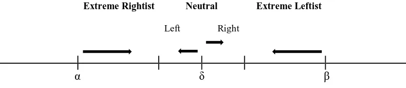
The political supports of different types of farmers with respect to subsidy level are summarized in the figure 3.

Figure 3. Farmers’ Political Supports Regarding the Subsidy Level

Due to the fact that getting the votes of extreme rightist farmers needs less subsidy than getting the neutral farmers and extreme leftist farmers, and getting the votes of neutral farmers needs less subsidy than getting the extreme leftist farmers, it is expected that α is lower than δ, and δ is lower than β. These threshold subsidy levels with respect to farmers’ political view can be mathematically illustrated as;

α < δ < β

In addition to these, the payoff functions of the rightist and leftist farmers do not only depended on the level of subsidy, but also the election results. Since people get happier and feel comfortable when their political view is in the power, the election results affect farmer’s utility as well. Therefore, the utility of seeing your political view in power can be defined as “p”. It means that if ruling party wins the election, while a leftist farmer can gets the only

Extreme Rightist Neutral Extreme Leftist

Left Right

(47)

subsidy (S), a rightist farmer not only benefits from the subsidy but also has a pleasure of winning the election (S, p). Therefore, utility functions of rightist and leftist farmers can be written as;

Uf (S, Y)

where S is the subsidy level, Y ∈ [0, p], and p is the pleasure of seeing your political view in power. By the way, a neutral farmer is only interested in the amount of subsidy he/she received, and the result of election neither benefits nor harms him/her. Hence, the utility function of neutral farmers can be showed as;

Uf (S)

Also, since subsidy level (S) is supposed to be a unit interval ranging from 0 to the 1, and p is discrete value whether 0 or p, the below inequalities can be deducted as;

Uf (S1, p) > Uf (S2, p) for all p and S1 > S2

Uf (S1, p) > Uf (S1, 0) for all S1

(48)

level which is not distributed to farmers (1 - S) is considered as a utility for a government in its payoff function. For example, if a government wins the election by offering S1 amount of

subsidy, the payoff of government becomes winning the election and the remaining amount of resource after giving the subsidy to the farmers (W, 1 - S). Thus, the utility functions for a government which are also shown in the related payoff functions can be written as;

Ug (X, 1 - S)

where X ∈ [ W, L] , and W and L stand for winning and losing an election, respectively and (1 – S) is the remaining amount of resource after giving the subsidy. Furthermore, due to the fact that the remaining amount of resource (1 – S) is supposed to be a unit interval ranging from 0 to the 1, and winning an election definitely is preferred to a losing an election, the below inequalities can be deducted.

Ug (W, 1 - S1) >Ug (W, 1 – S2) for allS2> S1

Ug (W, 1 - S1) >Ug (L, 1 – S2) for allS1 and S2

Ug (L, 1 - S1) >Ug (L, 1 – S2) for allS2> S1

(49)

In this context, a one-shot dynamic game with perfect information, and a two periods dynamic game with perfect information between government and farmers can be modelled. That is, players move in sequence, all previous moves are common knowledge before the next move, and the player’s payoffs are known. In these models, subsidies are given before the election is done. Furthermore, an alternative game theory model for agricultural subsidies among rightist party, leftist party and farmers can be analyzed where parties first announce a level of subsidy simultaneously, and the subsidy level offered by parties will be given conditional on winning the election.

6.1. A One-Shot Dynamic Game with Perfect Information

By combining all of the information so far, one-shot dynamic games for agricultural subsidy between policy makers and farmers can be formulated. In this one-shot game, the payoffs of the players are identified by the first election results. Since there are three types of region with respect to political views based on the previous election results and two types of region regarding the agricultural population (high and low), total 6 cases can be modeled by game theory approach.

6.1.1. Case 1: Extreme Rightist and High Agricultural Population Region

(50)

government (R) or the opposition party (L). Since the region is an extreme rightist region, it is considered that the ruling party polled greater than 50 percent of total votes in the last two elections in this region. Furthermore, since the region is extreme rightist and high agricultural population region, it is obvious that the political view of farmers in this region is extreme rightist.

Figure 4. Extensive–Form Representation of a Game for Case 1

(51)

That is, a government can win the election in an extreme rightist and high agricultural population region by offering any subsidy level. Additionally, since government’s utility decreases with a higher subsidy level, it will offer a subsidy level which is equal to zero. Therefore, even if the government does not give any subsidy in a high population extreme rightist region, it can win the election in a one-shot game. Intuitively, an inference can be drawn from this one-shot game that the threshold subsidy level of extreme rightist becomes zero (α=0) in an extreme rightist and high agricultural population region.

6.1.2. Case 2: Swing and High Agricultural Population Region

In this case, the region is swing, i.e., the winner party in the last two elections was not the same party. The rotation in the power was observed from rightist party to leftist party or vice versa. It means that there is not any dominant political view in this region, and the region is floating to the right or left party. Since the non-farmers are assumed to vote for the same party in every election, farmers need to be neutral voters. Also, the neutral farmers only benefit from the subsidy level, do not care whether current government wins the election or not. In other words, there is no utility with respect to seeing their political view in power for neutral farmers. Furthermore, the region has a high agricultural population which means that the number of farmers (voters) is equal and greater than the 50 percent of total voters in that region. Thus, the level of agricultural subsidy plays a crucial role to win an election in this region.

(52)

Figure 5. Extensive–Form Representation of a Game for Case 2

As shown in the Figure 5, there is a dynamic game with perfect information and the government moves first and then farmers take their decision. Government can set a subsidy level S, ranging from 0 to the 1. By observing the subsidy level, swing farmers votes for the government (R) or the opposition party (L).

(53)

In particular, they vote for the government party if and only if a subsidy level which is equal and greater than their threshold level.

Then, in this region the solution of the game is occurred at the payoff of {(W, 1 - δ), (δ)} where neutral farmers play R since the subsidy level offered by the government is equal to the threshold level of neural farmers. In other words, the government offers δ level of agricultural subsidy in order to win the game in a swing and high agricultural population region, and neutral farmers vote for rightist party.

6.1.3. Case 3: Extreme Leftist and High Agricultural Population Region

In this case, it is still a high agricultural region, i.e., the number of farmers (voters) is equal or greater than the 50 percent of total voters in that region. It means that farmers play a significant role in changing the political power. Furthermore, since the region is an extreme leftist region, it is considered that a ruling party polled lower than 50 percent of total votes in this region in the last two elections. From these information, it is clear that the political view of farmers is extreme leftist in this region.

(54)

In this region, the solution of the game is occurred at the payoff of {(L, 1 - S1), (S1, p)}

where extreme leftist farmers want to play L regardless of the government actions. As it is

shown in the payoff function, in a one-shot game playing L always give a higher payoff than playing R for an extreme leftist farmers, i.e., Uf (S, p) > Uf (S, 0) for all subsidy level.

Moreover, government prefers to play S1 because (L, 1 - 0) is better than (L, 1 - S) for all

subsidy level which is greater than zero. The solution of this one-shot game indicates that the rightist government always loses the election in an extreme leftist and high agricultural population region.

(55)

6.1.4. Case 4: Extreme Rightist and Low Agricultural Population Region

In Case 4, the region is a low agricultural population region which means that the number of farmers (voters) is lower than the 50 percent of total voters in that region. Therefore, farmers are not important in the political arena, their influence on the fate of election is very limited. Furthermore, the ruling party won the last two elections in this region. Then we can deduce that the non-farmers are rightist. Even though we could not know the political view of farmers in this case, without loss of generality we consider the case in which the farmers are extreme rightist. Hence, it is expected that government can easily win the election in this region without getting the votes of any farmers.

(56)

The extensive–form representation of a Game for Case 4 is shown in Figure 7, where government moves first and then farmers take their decision. Since regardless of the subsidy level proposed by the government, government can win the election government can offer a lower subsidy level which maximize its payoff. Thus, the solution of this game is occurred at the payoff of {(W, 1 - S1), (S1, p)} where government plays S1 and farmers plays R.

Additionally, since government’s utility decreases with a higher subsidy level, it will offer a subsidy level which is equal to zero (S1=0).

Like the solution of the case 1, even if the government does not give any subsidy in a low population extreme rightist region, it can win the election in a one-shot game. Although the solution of this game in case 4 and the solution of game in case 1 are the same, there are some differences between these two cases. First of all, the payoffs of the games are different, because in case 4 there is no way to lose an election for a current government. In addition to this, the government has a confidence in this region that it will win the election without taking account the farmer’s motive to vote for government. In other words, while the reason for government victory in case one is the farmer’s choice of voting R due to the utility of seeing their political view in power (p); on the other hand, it does not affect the outcome of the election in case 4.

6.1.5. Case 5: Swing and Low Agricultural Population Region

(57)

farmers in the eyes of politicians is not significant as much as in a high agricultural region. Besides, since the non-farmer population is more than 50 percent and their political view does not change based on the subsidy level, they give their votes to the same party in every election. Therefore, the party which gets the non-farmer’ votes wins the election. In particular, if the non-farmers are majority, the city will not be a swing city. That is, Case 5 will not be observed. For the completeness of our analysis, we provide the solution for this case even though it is impossible to observe it.

(58)

Since farmers are the minority in this region, they do not have any say on the results of the election. Hence, the subsidy level will not affect the election results. Government gives zero subsidy in this region. Since the zero is below the threshold, the farmers will vote for the opposition party.

In this situation, the votes of non-farmers can shape the results of the election in this region. If the majority of non-farmers’ population is leftist, the opposition party wins the election with 100 percentage votes in this region. If the majority of non-farmers’ population is rightist, the government will win the election by majority of votes. Therefore, the equilibrium outcome of this game, which depends on the political view of non-farmers population, is occurred at the payoffs of either {(W, 1 - S1), (S1)} or {(L, 1 - S1), (S1)} where S1 is equal to

zero.

6.1.6. Case 6: Extreme Leftist and Low Agricultural Population Region

(59)

is, Case 6 will not be observed. For the completeness of our analysis, we provide the solution for this case even though it is impossible to observe it.

As shown in the Figure 9, there is a dynamic game with perfect information and the government moves first and then farmers take their decision. Government can set a subsidy level S, ranging from 0 to the 1. By observing the subsidy level, farmers votes for the government (R) or the opposition party (L).

(60)

Like case 3, the solution of the game is occurred at the payoff of {(L, 1 - S1), (S1, p)}

where extreme leftist farmers want to play L regardless of the government actions. The solution

of this one-shot game indicates that a government always loses the election in an extreme leftist and low agricultural population region, whatever subsidy level it offers. The difference between case 3 and case 6 is that there is no chance to win the election for a government in an extreme leftist and low agricultural population region. In other words, whatever the farmers vote for, the opposition party wins the election in this region by giving zero subsidy.

6.2. Two Periods Dynamic Game with Perfect Information

After studying the one-shot game, two-period dynamic games for agricultural subsidy between policy makers and farmers can be modelled. In two-period dynamic game, there are two elections. After the first election, a government can stay in the power or an opposition party can come to the power. Besides, the definitions of the regions like extreme rightist, swing and leftist region may be changed based on the first election results. For example, if a current government loses the election in an extreme rightist region, then in the second election the region is considered as a swing region because of the changing the power from rightist to leftist party. Lastly, the payoffs of the farmers and parties are identified by the utility received by the first election and the discounted utility received by the second election. In other words, at the end of the two elections the total utility of farmers can be expressed as;

(61)

where U1f (S1, Y) is the farmers’ utility in the first period of the game, U2f (S2, Y) is the farmers’

utility in the second period of the game, k ∈ [0, 1] is the discount factor, and Y ∈ [0, p], and p is the pleasure of seeing your political view in power.

Furthermore, the assumptions made in one-shot game for the governments are also valid in two-period game. The payoff function of government certainly depends on the results of election and the subsidy level which is not distributed to farmers. If a government wins the first election, the total subsidy given to farmers in both electoral periods should be considered in the utility function of a government. On the other hand, if a government loses the first election, since it will not be in the power and offer any subsidy, only the subsidy given by in the first election is considered in its utility function. Therefore, for these two situations the utility functions for a government can be written as;

U1g (W, (1 – S1)) + kU2g (X, (1 – S2)) if government wins the first election,

U1g (L, (1 – S1)) if government loses the first election,

where (1 – S1) is the subsidy level which is not distributed to farmers in the first election, (1 –

S2) is the subsidy level which is not distributed to farmers in the second election, k is the

(62)

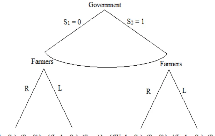
Figure 10. Extensive–Form Representation of a Two-Period Dynamic Game with Perfect Information

(63)

for the government (R) or the opposition party (L). After the election first election results, whether rightist government stays in power or a leftist government come to the power. Then again, rightist or leftist government set a subsidy level S, ranging from 0 to the 1, and then farmers votes for the current government or the opposition party.

Since there are three types of regions with respect to political views based on the previous election results and two types of region regarding the agricultural population (high and low), total 6 cases can be modeled by game theory approach.

6.2.1. Case 7: Extreme Rightist and High Agricultural Population Region

Based on our assumption, this region is composed of extreme rightist farmers, since rightist party won the election in the last two elections. As similar to the case 1, independent of who is government in the region and what subsidy level is offered, extreme rightist farmers votes for rightist party in the second period. In other words, the pleasure of seeing their political view in power gives them a higher utility. Therefore, the discounted utility that the farmers get in the second period of the game can be written as;

kU2f (S2, p)

where k is the discount factor and S2 is the subsidy level which current government (rightist

(64)

Situation 1: Rightist Government Wins the First Election

If a ruling party offers Sx level of subsidy before the first elections and wins the first

election, farmers have Sx level of subsidy and seeing their political view in power (p) in their

utility. After the first election, since government knows regardless of the subsidy level it will win the second election, it gives zero subsidy to maximize its utility. Therefore, if a government offers Sx level of subsidy in the first election and wins the both election, the total utility function

of farmers becomes as below;

U1f (Sx, p) + kU2f (0, p)

Situation 2: Rightist Government Loses the First Election

If a ruling party offers Sx level of agricultural subsidy before the first elections and

loses the first election, farmers have only Sx level of agricultural subsidy in their utility

function. After the first election, since the political power shifts from right to left, the region looks like swing region. Since the left government who comes to the power after first election considers the region as a swing region, it offers an agricultural subsidy which is equal to the threshold level of swing farmers. In other words, leftist government thinks that δ level of agricultural subsidy is sufficient to win the election. Therefore, if a rightist government offers Sx level of agricultural subsidy in the first election and loses the first election, then a leftist

(65)

U1f (Sx, 0) + kU2f (δ, p)

Comparison of Utilities: Situation 1 vs. Situation 2

In order to compare the farmers’ utility in Situation 1 and Situation 2, we should know the exact form of utility function of farmers. Without loss of generality, we take the utility function of farmers as a quasilinear function such as;

Uf (S, p) = S + Vf (p) where Vf (p) > Vf (0)

Based on our assumption on the farmers’ utility function, farmers will vote for the rightist party if below inequality holds.

Sx + Vf (p) + k(0 + Vf (p)) ≥ Sx + Vf (0) + k(δ + Vf (p))

Vf (p) ≥ Vf (0) + kδ

Otherwise, farmers vote for the leftist party if below inequality holds.

Sx + Vf (p) + k(0 + Vf (p)) < Sx + Vf (0) + k(δ + Vf (p))

Vf (p) < Vf (0) + kδ

(66)

a higher utility, farmers prefer to vote for rightist party. Since it is unclear, there is no unique solution for this two-period dynamic game in extreme rightist and high agricultural population region.

Note that the level of subsidy that the government gives in the first period does not play any role on the decision of the farmers. Hence, the government will give Sx=0 in the first

period. It is also worth noting that the election results in a one-shot game and two-period game in an extreme rightist and high agricultural population region may differ. In a one-shot game even though a government wins the election whatever he offers, in a two-period game it may lose the first election.

6.2.2. Case 8: Swing and High Agricultural Population Region

Based on our assumption, this region is composed of neutral farmers, since the government changed in the last two elections. Like Case 2, the region has a high agricultural population which means that the number of farmers (voters) is equal and greater than the 50 percent of total voters and there is not any dominant political view. Since the rightist government is in the power at the beginning of the first election and the region has a high agricultural population, it is possible that the non-farmers are rightist or leftist. However, since the majority is the farmers and the percentage of the votes does not affect the payoffs and the perception of the players, our analysis will be the same under both subcases.

(67)

Situation 1: Rightist Government Wins the First Election

If a ruling party offers Sx level of subsidy before the first elections and farmers vote for the

current government, the rightist government wins the first election by getting majority of the votes. After the first election, since current rightist government stays in the power, the region looks like an extreme rightist region in the perspective of the government. In other words, since the farmers are considered to be extreme rightist in this region, the rightist party will think farmers will vote for them independent of the subsidy level and offer a subsidy level equals to zero. Therefore, the total utility function of farmers becomes as below;

U1f (Sx) + kU2f (0)

Situation 2: Rightist Government Loses the First Election

If a ruling party offers Sx level of subsidy before the first elections and farmers vote

against the current government, the leftist government comes to the power. Since the region looks like a swing region, current leftist government think that a subsidy level which is equal to the swing farmers’ threshold level is sufficient to win the second election. Hence, farmers get δ level of subsidy in the second election and their total utility function becomes as below;

(68)

Comparison of Utilities: Situation 1 vs. Situation 2

It is obvious that farmers benefits more in the second situation. As shown in the below inequality, the utility received by the farmers in Situation 2 is always greater than the utility received in Situation 1.

U1f (Sx) + kU2f (δ) ≥ U1f (Sx) + kU2f (0)

U2f (δ) ≥ U2f (0)

To sum up, the actions taken by government and farmers can be explained as follows. Initially, government offers Sx level of agricultural subsidy, then neutral farmers vote against

the current government in the first election. Besides, since the rightist government knows whatever subsidy level it offers in the first election, the farmers will vote for the leftist party, it prefers to offer no subsidy (Sx=0) in the first elections to maximize its utility.

After the first election, the leftist party comes to the power and the region still looks like a swing region. Hence, leftist government offers δ level of agricultural subsidy, which is equal to the swing voter’s threshold level, and neutral farmers vote for the current leftist government in the second election. Therefore, the solution of the game is occurred at the below payoff.