ABSTRACT
XUE, SHANG. Genetic Architecture of Domestication and other Complex Traits in Maize. (Under the direction of James B. Holland and Jung-Ying Tzeng).
Research on domestication informs our understanding of the genetic architectures of
important traits and can guide efforts to identify causal genetic variants of crop. Numerous
morphological traits have changed during domestication from teosinte to maize. However,
standing variation still exists for several domestication-related traits in modern maize. The
genetic architecture for standing variation remaining in maize for these domestication-related
traits is unknown. In Chapter 2, the maize Nested Association Mapping population (NAM)
and a diversity panel were used to estimate the proportion of variation due to polygenic,
small-effect QTL versus larger effect variants; compare the genomic positions of larger effect
variants to the known locations of domestication; and partition the genetic variance using
variance components analysis methods. Additive polygenic models explained most of the
genotypic variation for domestication-related traits; no large effect loci were detected for any
trait. Previously defined improvement sweep regions were associated with more trait
variation than expected based on the proportion of the genome they represent. Small effect
polygenic variants (enriched in improvement sweep regions of the genome) are responsible
for most of the standing variation for domestication-related traits in maize.
Linear mixed models are widely used in humans, animals, and plants to conduct
genome-wide association studies (GWAS). Different from human datasets, experimental
units for plants are typically multiple-plant plots of families or lines that are replicated across
on plot-level data. Two-stage methods have been proposed to reduce the complexity and
increase the computational speed for GWAS. However, the appropriate dependent variable to
use in the second stage analysis and how to handle unbalanced datasets are not clear. In
Chapter 3, I developed a weighted two-stage analysis to reduce bias and improve power of
GWAS while maintaining the computational efficiency of two-stage analyses. Power and
false discovery rate of one-stage, different two-stage models and new weighted analysis are
compared by simulation based on real marker data of a diverse panel of maize inbred lines.
Only weighted two-stage GWAS has power and false discovery rate similar to the one-stage
analysis for severely unbalanced data in simulation. The weighted two-stage analysis method
was implemented in a free open source software TASSEL.
Genetic diversity reduced severely due to selection and bottleneck effect during
domestication of maize from teosinte. However, the gene pool of teosinte might harbor
agriculturally beneficial alleles. Due to their linkage with a genomic background that is
unadapted, measuring the potential benefit of teosinte alleles is challenging. A population
called the ZeaSynthetic population was developed as a bridge to investigate teosinte specific
alleles in a common maize background. Genotypes of 1846 parents were obtained by
genotyping by sequencing and phenotypes of 923 pairs of S1 and S0 full-sib progeny
families were measured across six environments. Due to unusual population structure and
experimental design, there is no ready to use software available for analysis. In Chapter 4, I
used a linear mixed model to estimate additive and dominance effects at each SNP and used
simulation to evaluate power and bias of genetic effect estimates from this model. Simulation
results showed that the linear mixed model is a reasonable model with low bias estimating
with rare alleles and loci in lower recombination regions of the genome tend to have larger
additive and dominance effects. These results suggest that recessive deleterious alleles tend
to be concentrated in lower recombination regions, and that favorable alleles for agriculture
are more likely to be at higher starting frequencies and found at loci in higher recombination
© Copyright 2017 Shang Xue
Genetic Architecture of Domestication and other Complex Traits in Maize
by Shang Xue
A dissertation submitted to the Graduate Faculty of North Carolina State University
in partial fulfillment of the requirements for the degree of
Doctor of Philosophy
Bioinformatics
Raleigh, North Carolina
2017
APPROVED BY:
_______________________________ _______________________________
James Holland Jung-Ying Tzeng
Committee Co-Chair Committee Co-Chair
_______________________________ _______________________________
ii
DEDICATION
To my parents, for providing love, care, support and encouragement for over twenty
years. Thanks for giving me healthy body and free mind, so that I can explore new
knowledge in new environment.
谨以此文献给我的父母,感谢你们给予我二十多年的关心和爱护,支持和鼓励。感谢
iii
BIOGRAPHY
Shang Xue was born on October 7, 1991 at a small town in Linyi, China. She
graduated from Shandong University with Bachelor of Science in Biological Science. During
the undergraduate study there, she was attracted by amazing genetics and the power of
computer to analyze genomic data. Later she came to the U.S. in 2012 as a Ph.D. graduate
student in Bioinformatics at North Carolina State University to continue exploring new
techniques in the field of genomics. She met great advisors and instructors there, and
enjoyed both her study and life. After graduation, she will work as a bioinformatician at a
technology company and she is looking forward to use the knowledge she learned to make
iv
ACKNOWLEDGMENTS
There are so many people that influenced my academic life and personal life. First, I
would like to especially thank my Ph.D. advisor, Dr. Jim Holland. Along the way, you gave
me tremendous help and endless patience in my research. You are not only providing me
academic guidance, but also setting an inspiring example for personal life and future career.
Great thanks also go to my co-advisor, Dr. Jung-Ying Tzeng. You gave me solid support on
statistical analysis and taught me how to solve problems with rigorous attitude. Your patience,
thoughtfulness, solicitude, encouragement brought warmth to my overseas graduate life and
your professionalism impacted my academic life profoundly. All those good qualities you
gave me will keep motivating me to work harder and explore bigger world as a foreign
scholar.
Thanks also go to other advisory committee members, Drs. Alison Motsinger-Reif
and Ross Whetten, for providing me comments and suggestions. Many numbers of Holland
Lab have contributed their insights into this dissertation including: Drs. Bode Olukolu, Funda
Ogut, Charlie Zila, Tiffany Jamann, Zhou Fang, Luis Fernando Samayoa, Jeffrey Dunne and
Ryan Andres; technicians, Jason Brewer and Josie Bloom; and graduate students, Thiago
Marino, David Horne, Matthew Smith and Anna Rogers. I also want to thank Drs. Qin Yang,
Peter Balint-Kurti, Peter Bradbury, Ed Buckler, Brian Reich, Howard Bondell, Sherry A.
Flint-Garcia and Ginnie Morrison for suggestions and collaborations.
I want to say Thank You to my mom and dad for training my tenacity, patience,
curiosity and positive attitude since I was a child. Those good qualities lead me through the
v Finally, thanks all my friends for sharing joys and tears, your support and
vi
TABLE OF CONTENTS
LIST OF TABLES ... viii
LIST OF FIGURES ... ix
CHAPTER 1: Literature Review ... 1
Maize domestication ... 1
Maize improvement from breeding ... 5
Genetic architecture of complex traits in maize ... 7
Methods and populations used for complex trait genetic analysis in maize ... 10
Frontiers of complex trait genetic analysis in maize... 15
References ... 25
CHAPTER 2: Genetic architecture of domestication-related traits in maize ... 35
Abstract ... 37
Introduction ... 39
Material and Methods ... 44
Results ... 56
Discussion... 62
Figures and Tables ... 67
References ... 78
CHAPTER 3: Comparison of one-stage and two-stage genome-wide association studies ... 83
Abstract ... 85
Introduction ... 86
Material and Methods ... 93
Results ... 101
Discussion... 106
Figures and Tables ... 113
References ... 121
CHAPTER 4: Genomic distribution of deleterious recessive variation in the ZeaSynthetic population ... 125
Abstract ... 127
Introduction ... 128
vii
Results ... 143
Discussion... 146
Figures ... 150
References ... 159
APPENDICES ... 163
APPENDIX A: Supplemental Material for Chapter 2 ... 164
APPENDIX B: Supplemental Material for Chapter 3 ... 180
viii
LIST OF TABLES
Table 2.1. Summary statistics and heritability estimates (ℎ2) for three domestication-related
traits: shank length (SL), cob length (CL), kernel row number (KRN) in the maize NCRPIS
diversity and NAM panels. ... 74
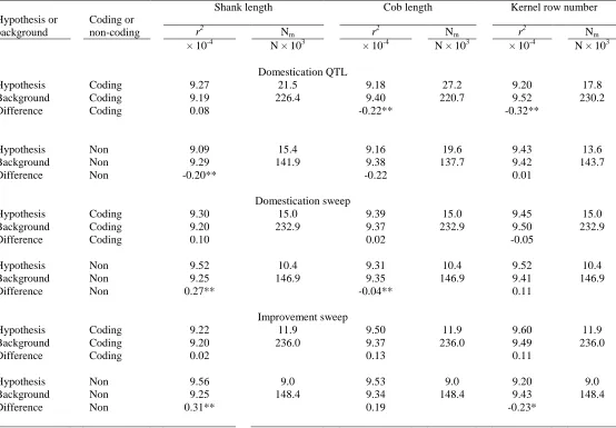
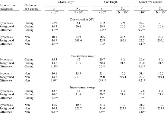
Table 2.2. Mean SNP association r2 and number of markers (Nm) inside and outside
hypothesis-defined testing regions in NCRPIS panel. ... 75
Table 2.3. Mean SNP association r2 and number of markers (Nm) inside and outside
hypothesis-defined testing regions in NAM panel... 76
Table 2.4. Tests of associations between haplotypes of known domestication genes and
domestication-related traits in NCRPIS panel. ... 77
Table 3.1. Parameter settings for simulation study. ... 118
ix
LIST OF FIGURES
Figure 2.1. Distribution of shank length, cob length, kernel row number and masculinized ear
tip length in NCRPIS panel (red) and NAM population (green). ... 67
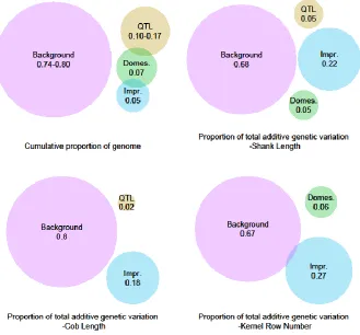
Figure 2.2.A. The proportion of variance for shank length, cob length, and kernel row
number among inbred lines of the NCRPIS panel associated with relationship matrices based
on all SNPs in hypothesis-defined regions or on background SNPs. ... 68
Figure 2.2.B. Cumulative proportion of genome tagged by SNPs defining hypothesis
relationship matrices and background matrices, and the proportion of total additive genetic
variation associated with each relationship matrix for shank length, cob length, and kernel
row number among inbred lines of the NCRPIS panel... 69
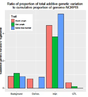
Figure 2.2.C. Ratio of proportion of total additive genetic variation to cumulative proportion
of genome tagged by SNPs defining hypothesis and background relationship matrices for
shank length, cob length, and kernel row number among inbred lines of the NCRPIS panel. ... 70
Figure 2.3.A. The proportion of variance for shank length, cob length, and kernel row
number among inbred lines of the NAM panel associated with relationship matrices based on
all SNPs in hypothesis-defined regions or based on background SNPs. ... 71
Figure 2.3.B. Cumulative proportion of genome tagged by SNPs defining hypothesis
relationship matrices and background matrices, and the proportion of total additive genetic
variation associated with each relationship matrix for shank length, cob length, and kernel
x Figure 2.3.C. Ratio of proportion of total additive genetic variation to cumulative proportion
of genome tagged by SNPs defining hypothesis and background relationship matrices for
shank length, cob length, and kernel row number among inbred lines of the NAM panel. ... 73
Figure 3.1. Power of six different association testing methods to detect causal variants for
three different genetic architectures and three levels of data imbalance. Balanced datasets had
all lines evaluated at all environments with no missing values (24800 records). Randomly
unbalanced datasets contained a random subset of 50% of the data of the complete dataset
(12400 records). Severely unbalanced datasets had half of the lines evaluated at only one
environment and the other half of lines evaluated at ten environments (13640 records). ... 113
Figure 3.2. False discovery rate when false positives were defined as markers that had LD r2
< 0.1 with true QTL and were declared significant at the empirically estimated q < 0.05.
False discovery rate is the proportion of false positives defined this way among all markers
declared significant. False discovery rate for residual 3-step method is not shown, since it
identified very few significant markers. ... 114
Figure 3.3. False discovery rate when false positives were defined as markers that had LD r2
< 0.05 with true QTL and were declared significant at the empirically estimated q < 0.05.
False discovery rate is the proportion of false positives defined this way among all markers
declared significant. False discovery rate for residual 3-step method is not shown, since it
identified very few significant markers. ... 115
Figure 3.4. Distributions of all genome-wide marker association test p-values using the
one-step analysis (Y-axis) or two-one-step analysis (X-axis) for three different genetic architectures
and three levels of data imbalance. P-values from weighted BLUE two-stage method are in
xi Figure 3.5. Bias of QTL effect estimates from different GWAS methods for three different
genetic architectures and three levels of data imbalance. ... 117
Figure 4.1. Bias of additive effect estimates under 12 different simulation scenarios. Bias was
calculated as the mean of estimated values minus the true simulated effect at simulated QTL.
Bias is reported as a proportion of the true causal effect. DAratio is ratio of the simulated
dominance effect to the additive effect. 0.25 SD, 0.5 SD, 1 SD are simulated additive effect
size and SD is the standard deviation of phenotypic value of the corresponding trait. ... 150
Figure 4.2. Bias of dominance effect estimates under 12 different simulation scenarios. Bias
was calculated as the mean of estimated values minus the true simulated effect at simulated
QTL. Bias is reported as a proportion of the true causal effect. DAratio is the ratio of the
simulated dominance effect to additive effect. 0.25 SD, 0.5 SD, 1 SD are simulated additive
effect size and SD is the standard deviation of phenotypic value of the corresponding trait. .... 151
Figure 4.3. Power of detecting QTL under 12 different simulation scenarios. DAratio is the
simulated dominance effect to additive effect ratio. 0.25 SD, 0.5 SD, 1 SD are simulated
additive effect size and SD is the standard deviation of phenotypic value of the corresponding152
Figure 4.4. Relationship between standardized additive effect (X-axis) and standardized
dominance effect (Y-axis) for SNPs with MAF below 0.1. Standardized genetic effect is
genetic effect estimate divided by its corresponding standard error. ... 153
Figure 4.5. Relationship between standardized additive effect (X-axis) and standardized
dominance effect (Y-axis) for SNPs with MAF above 0.3. Standardized genetic effect is
genetic effect estimate divided by its corresponding standard error. ... 154
Figure 4.6. Relationship between absolute value of standardized additive effect (Y-axis) and
xii Figure 4.7. Relationship between absolute value of standardized dominance effect (Y-axis)
and MAF (X-axis) ... 156
Figure 4.8. Relationship between absolute value of average standardized additive effect
(Y-axis) and recombination rate (X-(Y-axis) ... 157
Figure 4.9. Relationship between absolute value of average standardized dominance effect
1
CHAPTER 1: Literature Review Maize domestication
The domestication of all major crop plants occurred in a relatively short period in
human history starting about 10,000 years ago (Harlan 1992). Crop domestication occurred
when humans began to selectively save and replant seeds of preferred forms from wild
species. Plant attributes that humans preferred in crops are referred to as the domestication
syndrome (Hammer 1984; Harlan et al. 1973). The attributes include reduced number of
harvest units (ears in the case of maize), suppression of shattering (seed dispersal), and larger
seed size. Maize (Zea mays ssp. mays) was domesticated from its progenitor teosinte (Z.
mays ssp. parviglumis) about 6000 to 10000 years ago in southern Mexico (Galinat 1983;
Iltis 1983; Matsuoka et al. 2002; Piperno et al. 2009; van Heerwaarden et al. 2010).
The process of domestication involved artificial selection that resulted in radically
different floral, ear, and kernel morphologies between teosinte and maize (Beadle 1939;
Doebley et al. 1990; Doebley and Stec 1993; Iltis 1983). Teosinte plants have elongated
lateral branches at many nodes. In contrast, maize plants typically produce a lateral branch at
only two or three of the nodes on their main stems, and these are much shorter than teosinte lateral branches, being reduced to a “shank” that terminates at the base of a female ear
(Doebley et al. 1997). Furthermore, teosinte “ears” are small, with kernels arranged in a
distichous (two-ranked) pattern on the ear axis, compared to large ears of maize that typically
have from eight to over twenty rows of kernels in four or more ranks. Several major QTL and
in some cases, the specific genes, controlling these differences between maize and teosinte
2 Genetic bottlenecks due to domestication
As a consequence of artificial selection, alleles favorable for growth and development
under agricultural conditions or for other traits desired by humans (such as flavor) increased
in frequency, often reaching fixation and reducing genetic variation very near causal
sequence sites (Wang et al. 1999). In addition, domestication was often accompanied by
severe genetic bottlenecks from the use of small founder populations. The strong directional
selection that occurred during the domestication of maize from teosinte reduced genetic
diversity most strongly at key genes controlling domestication-related traits. Similar to other
crops, previous studies have demonstrated that lower levels of genetic diversity among
inbreds than among landrace and teosinte populations are caused by selection and
demography (bottlenecks) (Tenaillon et al. 2004; Wright et al. 2005). Estimates of the
amount of diversity lost are generally agreed to be around 30% in maize (BUCKLER et al.
2001; Zhang et al. 2002). This is similar to other grass species, such as rice (29% reduced;
Oka 1988) and sorghum (33% reduced; Morden et al. 1990). Additional studies indicated
that approximately 2 to 4% of genes (500 to 1000 genes) were targets of artificial selection
during domestication and breeding (Hufford et al. 2012; Wright et al. 2005).
Domesticated plants can be model systems to study the genetic basis of adaptation, in
which human artificial selection was imposed in addition to natural selection (Brown 2010;
Ross-Ibarra et al. 2007). Also, understanding crop origins and domestication can contribute
to the identification of useful genetic resources for breeding (HARRIS 1990; Olsen and
Wendel 2013). By influencing the levels of nucleotide diversity and patterns of linkage
3 Research on domestication also informs our understanding of the genetic architectures of
important traits and can guide efforts to identify causal genetic variants of crop.
Standing variation in maize for domestication-related traits
Despite the severe bottleneck that occurred during domestication and strong selection
for the maize plant type, standing variability in cob length, kernel row number, and shank
length can still be observed among maize breeding lines. In addition, although most maize
plants have purely female flowers on their lateral branch termini, some lines of maize
produce a spike of staminate florets at the tips of their ears (Holland and Coles 2011),
referred to as “masculinized ear tips”, revealing variation for this domestication trait as well.
The genetic architecture for standing variation remaining in maize for these
domestication-related traits is unknown. Sequence variation at the same set genes that were
involved in the conversion of teosinte into domesticated maize may cause some portion of
this variation. Several large-effect mutations that cause maize to exhibit teosinte-like
morphological characteristics, such as tb1 and gt1, were later demonstrated to be allelic to the
corresponding domestication loci (Doebley et al. 2006; Studer et al. 2011; Wills et al. 2013).
Not all domestication alleles are fixed in domesticated species (Meyer and Purugganan 2013;
Studer et al. 2011), leaving open the possibility that some domestication loci contribute to
standing trait variation in domesticated species. Furthermore, a range of allelic series exists at
some domestication loci (Studer and Doebley 2012); smaller-effect alleles may segregate in
domesticated species even if larger-effect wild-type alleles were lost from the species.
4 domestication bottleneck because of lower selection intensity or may have arisen by mutation
after domestication.
Alternatively, the observed phenotypic variation for domestication traits within
domesticated species might be due to large-effect genes that are distinct from the known
domestication genes. The variants at these genes may have arisen after domestication, or had
effects sufficiently small as to avoid purging during domestication. A third possibility is that
the observed phenotypic variation for domestication traits is produced by many small-effect
variants distributed throughout the genome, resulting in a polygenic genetic architecture.
Even if major-effect alleles were fixed during domestication, smaller-effect variants at other
loci could cause phenotypic variation in domestication target traits. Again, these variants
could have existed in the wild ancestor and passed through the domestication bottleneck due
to small selection coefficients, or they may represent new variation that arose from mutation
following domestication.
Loss of useful alleles during domestication?
Because selection and bottleneck effects have greatly reduced the genetic diversity
among modern maize varieties, some alleles segregating in teosinte did not pass through the
domestication bottleneck and do not exist in maize. It is likely that at least a small proportion
of these teosinte-specific alleles could have favorable effects if transferred to maize; they
could have been lost from maize populations simply by random genetic drift due to the
population bottlenecks in domestication. Teosinte populations may harbor unique alleles for
disease resistance other useful agricultural traits that could be used for plant breeding and
5 however, because of the numerous dramatic morphological between maize and teosinte.
Phenotypic comparisons between the subspecies will not reveal useful teosinte alleles
because they are completely confounded by the agronomically unacceptable wild plant
growth habit, morphology, and seed dispersal phenotypes. Furthermore, teosintes are not
adapted to temperate growing environments and will not flower under long daylengths of the
USA Corn Belt growing season(Hung et al. 2012). Therefore, alleles in teosinte that affect
productivity are completely masked by the expression of flowering repressors in teosinte. For
these reasons, specialized experimental populations derived from crossing between teosinte
and maize parents are required to estimate the effects of teosinte-specific alleles in the
context of the maize genome, morphology, and modern agricultural management and
production methods.
Maize improvement from breeding
From population improvement to inbred-hybrid breeding
Following the domestication of maize in Southern Mexico, humans spread maize
from its center of origin and selected for desired forms adapted to dramatically different
ecological conditions and for different uses. Maize was spread from Canada to Chile by
humans before the arrival of Europeans in the New World (Weatherwax 1954). The result of
this spread and divergent selection process over thousands of years is a dramatic variation in
many observable phenotypes in maize. Subsequent classification of the sub-populations of maize based on their geography and morphology recognized up to 350 distinct ‘races’ of
6 1988; Goodman et al. 1988; Vigouroux et al. 2008). Different maize races are adapted to
widely different ecological conditions (Ruiz Corral et al. 2008).
Since maize is naturally an open-pollinated crop, the traditional populations grown in farmer’s fields represent highly variable segregating populations with dynamic genetic
characteristics influenced by natural selection for adaptation, human selection for appearance
and various uses, and migration due to intentional seed exchange as well as to pollen spread.
Due to various individual preferences, production conditions, and production objectives from one farming household to another, farmers’ widely observed practice of selecting and saving
seed from the previous harvest and occasionally exchanging seeds provided the basis for the
initial pool of diverse and locally-adapted maize varieties (Badstue et al. 2007; Pressoir and
Berthaud 2004).
The earliest scientific breeding efforts in maize were aimed at improving populations
through selection on individual plants or seeds. Starting in the 1920s, efforts began to exploit
the strong hybrid vigor, or heterosis, of maize, by breeding inbred lines and crossing
unrelated inbred lines to produce hybrid varieties (Duvick et al. 2010). This method was
ultimately highly successful, resulting in nearly complete adoption of hybrid maize varieties
by farmers by 1970, and tremendous gains in average yield per hectare of maize in the USA.
The effect of this intensive breeding effort is a second phase of reduction in allelic diversity between modern maize inbreds and older outcrossing “landrace” maize populations on top of
the loss of diversity due to domestication. This more recent loss of diversity has been referred to as the “improvement bottleneck” and signals of particularly strong selection above the
background level of diversity reduction have been observed at numerous genome regions
7 Modern maize breeders recognize different sub-groups of maize breeding lines
referred to as “heterotic groups”. A heterotic group is a set of lines related by pedigree that
when crossed together will express only limited heterosis. Crosses between heterotic groups,
however, express substantial heterosis. Therefore, maize breeders tend to repeatedly cross
lines within heterotic groups to produce new breeding lines, whereas they cross lines between
heterotic groups to produce hybrid varieties that farmers grow (Tracy and Chandler 2006).
The result of this repeated recycling of related lines within heterotic groups has been a strong
divergence of allele frequencies genome-wide between the heterotic groups (van
Heerwaarden et al. 2012).
Genetic architecture of complex traits in maize
Inbreeding depression and heterosis
Although the inbred-hybrid method is almost universally accepted as the best
breeding method for improving yield in maize, the initial phases of the inbred-hybrid
breeding method were not entirely promising because of the strong inbreeding depression
that occurred during the process of repeated self-fertilization out of the original
open-pollinated source populations. Inbreeding depression refers to the reduced survival and
fertility of offspring of related individuals, it occurs in wild animal and plant populations as
well as in humans, indicating that genetic variation in fitness traits exists in natural
populations (Charlesworth and Willis 2009). Heterosis refers to the phenomenon that
progeny of diverse varieties of a species or crosses between species exhibit greater biomass,
8 outcrossing is the converse of inbreeding depression. Because intercrossing inbred strains
improves yield (heterosis), which is important in crop breeding, the genetic basis of these
effects has been debated since the early twentieth century.
There are two primary hypotheses about the genetic mechanisms responsible for
heterosis and the success of maize hybrids. First, overdominance models of heterosis predict
that at a single locus two distinct alleles confer heterozygote advantage when combined.
Alternatively, the dominance model predicts that heterosis is driven by dominance effects
and the complementation of favorable alleles in repulsion-phase linkage, particularly in low recombination regions (which can generate “pseudo-overdominance” in the absence of true
overdominance) (Gerke et al. 2015; Hill and Robertson 1966; McMullen et al. 2009). The
majority of genetic evidence indicates that the dominance model can explain most of the
genetic control of inbreeding depression and heterosis (Crow 2000; Gardner and Lonnquist
1959; Gerke et al. 2015; Mezmouk and Ross-Ibarra 2013; Moll et al. 1963), although there is
still some debate (Birchler et al. 2010). It is important to understand genetics underlying
inbreeding depression and heterosis to design optimal breeding strategies for hybrid crops. If
loci with heterozygote advantage are common, artificial selection in agricultural species
should select for strains that manifest substantial heterosis. Crop plants with a uniform,
highly heterozygous genotype with high fitness could be desirable, and could perhaps be
achieved by asexual seed production (Grossniklaus et al. 2001). However, if heterosis in
crops is mainly caused by complementation of dominant favorable alleles that mask
deleterious mutations, it might be better to exclude these alleles to produce high-yield
9 address the question of why genetic variation in fitness-related characteristics exists in so
many species, including humans (Lewontin 1974).
Recombination rate and genetic load
Recombination has large impact on evolution in general and plant breeding in
particular by promoting the diversity necessary to respond to continually changing
environments and preventing the build-up of genetic load by decoupling linked deleterious
and beneficial alleles. Recombination varies among genomic region in both animal and
plants (Anderson et al. 2001; Gaut et al. 2007; Jensen-Seaman et al. 2004) and variation in
recombination rates may be associated with the distribution of variants for genetic load or
inbreeding depression. There are two main reasons for varying crossover rate at the
molecular level. First, the chromatin structure heavily influences recombination rates in
plants. Heterochromatic regions generally reduce crossovers, however, knockout of
cytosine-DNA-methyl-transferase (MET1) resulted in genome-wide CpG hypomethylation and
increased the proportion of crossovers (Colome-Tatche et al. 2012; Mirouze et al. 2012;
Yelina et al. 2012). Fu et al.(Fu and Dooner 2002) demonstrated that, in maize, crossovers
were suppressed in regions with repetitive DNA sequences derived from retrotransposons
compared to sequences including and nearby functional coding gene sequences. Highly
repetitive retrotransposon-derived sequences tend to be heterochromatic in maize(Slotkin and
Martienssen 2007). Second, nucleotide content may also be associated with recombination
rate possibly due to the effect of GC-biased gene conversion (bGC)(Serres-Giardi et al.
2012). Maize experienced a modest bottleneck in genetic diversity (Tenaillon et al. 2004),
10 leading to the founder lines, many weakly deleterious alleles can be found segregating at low
frequencies among inbreds (Mezmouk and Ross-Ibarra 2013).
McMullen et al. (McMullen et al. 2009) observed that excess residual heterozygosity
was enriched in pericentromeric regions of maize inbred lines, suggesting that selection
against deleterious recessive alleles has been less efficient in these regions because of
reduced recombination frequency, as predicted by the Hill-Robertson effect (Hill and
Robertson 1966). In addition, other studies observed that deleterious alleles enriched in
low-recombination regions, as expected because reduced low-recombination permits deleterious
alleles to hitchhike to high frequency during selective sweeps (Hartfield and Otto 2011;
Rodgers-Melnick et al. 2015). However, a recent study shows that putatively deleterious
nonsynonymous polymorphisms in maize were not significantly enriched in regions of low
recombination (Mezmouk and Ross-Ibarra 2013).
Methods and populations used for complex trait genetic analysis in maize
Understanding gene to phenotype relationships and discovering genes affecting
agronomic traits has great value for increasing the speed of selective breeding programs in
agriculturally important plants and animals and for predicting adaptive evolution. The
discovered association can be used for marker assisted selection (Collard and Mackill 2007),
genomic prediction (Bian and Holland 2017; Spindel et al. 2016) and understanding genetic
architecture for agriculturally important traits (Buckler et al. 2009; Kump et al. 2011; Poland
et al. 2011). However, most important agronomic traits are complex: they are quantitative
11 environmental factors, and interactions between genes and the environment. Pinpointing the
causal genes underlying quantitative trait loci (QTL) for complex traits can be challenging,
and the difficulties are greater as the proportion of phenotypic variance caused by a gene are
smaller.
Linkage analysis and association mapping are two important approaches for QTL
mapping. Linkage mapping in biparental crosses was the classical approach for QTL
mapping in plants; by relying on recent recombination events, it has the advantage of
requiring fewer genetic marker to cover the genome and high statistical power per allele
(Mauricio 2001)(Doerge 2002). However, it has limitations, including the substantial work
required to build mapping populations, limited sampling of allelic variability, and low
mapping resolution (Mauricio 2001). The development of high-throughput, dense genotyping
has led to a shift from traditional QTL mapping to association or LD mapping to overcome
these limitations (Zhu et al. 2008). Rather than focusing on two parental lines that differ
strongly in phenotype, LD-mapping approaches assess the correlation between phenotype
and genotype by taking advantage of LD in populations of unrelated individuals (Morrell et
al. 2012; Myles et al. 2009). First, by relying historical recombination event in natural
population, association mapping surveys genetic variation in much larger genetic pools than
a biparental cross (Myles et al. 2009). Second, it eliminates the time and effort required to
create specialized mapping populations because association mapping can be conducted in
general populations (Nordborg and Weigel 2008). Thirdly, it allows for high resolution for
QTL mapping, potentially to the level of causal nucleotide variants, depending on the extent
12 Association analysis has limitations as well, in particular the need to correct for
population structure effects that can lead to false positives, and lower power to detect
relatively rare variants. Previous results showed that genome wide association studies
suffered from low power (Asimit and Zeggini 2010; Gibson 2012; Korte and Farlow 2013)
and failing to explain missing heritabilities (Eichler et al. 2010; Li et al. 2010; Manolio et al.
2009). Most GWAS studies started first by identifying SNPs that segregate at intermediate
frequency in a small population; then SNPs are genotyped in larger samples and phenotypes
are measured. The underlying motivation is the assumption that common phenotypic
variation will be caused by common genetic variation. In the context of human genetics, this
assumption is known as the common disease-common variant hypothesis (Lander 1996).
Although thousands of significant associations have been found, they explained low percent
of variation of phenotypes (Eichler et al. 2010; Manolio et al. 2009). GWAS studies in plants
in some cases have been more successful than in humans (Brachi et al. 2011), however, the
missing-heritability issue still occurs (Li et al. 2010).
Variance component partitioning can be used as a complementary approach to
GWAS to assess enrichment of significant associations of a particular genomic regions or
functional class. Previous association studies showed that there is enrichment for significant
trait associations in coding regions and UTRs compared to intergenic SNPs (Schork et al.
2013). Although it is possible to document relative enrichment of associations in particular
genome regions, this can be confounded by correlations among SNPs in different regions.
Furthermore, the contribution of different categories of sequence variants to trait heritability
cannot be determined from GWAS. To address these limitations variance component analysis
13 collectively by groups of SNPs (Cross-Disorder Group of the Psychiatric,Genomics
Consortium 2013; Gusev et al. 2013; Lee et al. 2012; Lee et al. 2011; Speed et al. 2012;
Yang et al. 2013; Yang et al. 2010; Yang et al. 2011; Zaitlen and Kraft 2012; Zaitlen et al.
2013). In contrast to genome wide association study, variance components analysis leverages
the entire polygenic architecture of each trait and accounts for pervasive linkage
disequilibrium (LD) across functional categories. For a single component of genotyped (or
imputed) SNPs, h2 is defined as r2 between the true phenotype and the best linear prediction over those SNPs. With multiple components, the goal of the partitioned analysis is to
quantify the h2 directly explained by SNPs in each functional category while excluding tagging of SNPs in other categories. Thus h2 for each functional category is defined as the r2 between the true phenotype and the prediction only from SNPs in that functional category
when all functional categories are jointly analyzed for a best linear prediction. First, SNPs are
grouped into different categories according to functional annotation, then genetic relationship
matrices (GRM) for SNPs in each category are calculated. The total variance of the
phenotype can be modeled as a summation of variance component multiplied by its
corresponding GRM. Then h2 for each category can be calculated after obtaining variance components estimates. Simulation showed that this approach provides accurate genome-wide
estimates of heritability in diverse genetic architectures (Gusev et al. 2014; Lee et al. 2011).
Numerous association mapping panels are already available in maize (Crouch et al.
2011). The largest and most diverse such population that is publicly available is a set of
2,815 inbred lines maintained by the U.S. Department of Agriculture North Central Region
Plant Introduction Station (NCRPIS) (Romay et al. 2013). This collection contains lines
14 and has been densely genotyped (Romay et al. 2013). An alternative to conducting
genome-wide association study in samples of breeding lines, which are characterized by complex
population structure, is to use multiple parent populations of known pedigree, with known
population structure. One such population is the maize Nested Association Mapping (NAM)
population, which consists of 4892 recombinant inbred lines (RILs) derived from 25
bi-parental families (Buckler et al. 2009; Hung et al. 2012; Tian et al. 2011; Yu et al. 2008).
High resolution GWAS can be conducted in NAM while controlling for the known pedigree
structure and for genetic variation at unlinked QTL detected by joint multiple population
linkage analysis (Kump et al. 2011; Tian et al. 2011). For diverse maize germplasm sample,
most alleles have low frequency (Romay et al. 2013). Association mapping in diversity panel
relies on natural historical recombination, which has produced reshuffled genomes with
relatively short blocks of LD, providing high power for detection of QTL effects. Whereas
diversity panels can be obtained directly from seed banks, the NAM population required
substantial resource investment to generated thousands of lines by controlled pollinations
over several generations. The NAM provides the advantage that frequencies of alleles
captured in the parents are balanced in the progeny, the population structure is known, and
LD decay is intermediate between a diversity panel and a single biparental cross, resulting in
high of power and moderate resolution for QTL detection.
The relative ease of controlled matings in maize permits the development of
specialized experimental populations that can combine the high resolution of diversity panels
with low levels of population structure. An example of such a population is the recently
developed maize ZeaSyn 6 population. ZeaSyn6 was developed by introgressing teosinte
15 random mating in the generating process, this population has reduced LD and essentially no
population structure. Because of the population makeup, this population contains a large
proportion of moderately rare alleles, and can serve as a useful and unique tool to investigate
teosinte-specific rare alleles.
Frontiers of complex trait genetic analysis in maize
Comparing results from different methods and population types.
Little work has been done to apply variance component partitioning approaches to
address biological hypotheses in plants. Even in human genetics studies, where such methods
were pioneered, the results were presented in isolation of GWAS studies. An important
objective for contemporary quantitative genetics analysis is the implementation of variance
component partitioning analysis on the same data sets as GWAS methods, and comparisons
of the results.
GWAS can identify markers linked to individual or clustered sequence variants that
have relatively large effects on phenotypes. However, when effect sizes at individual SNPs
are so small that they do not pass genome-wide significance thresholds in GWAS or when
causal variants are not in sufficiently LD with available SNPs, GWAS will not detect these
SNPs or attribute any proportion of the heritability to them (Lee et al. 2011). As a
complementary approach, both real data analysis and simulations demonstrated the value of
the variance-component approach in recovering true additional heritability beyond that
explained by individually or jointly significant markers in various disease traits (Yang et al.
16 Psychiatric,Genomics Consortium 2013).Therefore, findings combining GWAS analysis and
variance components analysis can provide important ramifications for fine-mapping study
design and understanding of complex disease architecture.
In addition, no formal tests of significance have been developed for determining if a
particular class of variants explain more variation than expected by chance. Such tests are
hindered by the complex dependencies between different features of the genome, such that
variation attributed to one class of variants may in fact be due to another class with which it
is correlated. To address this problem, in Chapter 2 of this thesis, I developed several
strategies to estimate the expected variation for random sets of SNPs using resampling
methods and simultaneous fitting of covariance matrices defined for different sets of variants.
It will also be important to compare genetic architecture results across populations
with different structure and composition. In Chapter 2 of this thesis, I applied both variance
component partitioning and GWAS to both a multiparent linkage mapping population (the
maize nested association mapping population) and a very genetically diverse panel of inbred
lines representing most of the inbred maize line collection of the USDA seed bank. This
permitted comparisons of results of very different methods across two populations with
contrasting levels of diversity, allele frequency distributions, population structure, and
linkage disequilibrium.
Two-step GWAS algorithms
Using a linear mixed model that accounts for extraneous factors and genetic
background effects to estimate a single SNP effect can be computationally challenging for
17 proposed in human, animal and plant studies to speed up this process. The stage-wise
approach is often used where the raw phenotypes are first adjusted by extraneous effects
before analyzing them with a linear mixed model in the second step. In human studies,
two-stage regression analysis is often used to test SNPs for associations with quantitative diseases
(Laird et al. 2000; Naylor et al. 2009; Zeegers et al. 2004). The limitations are biased
estimates of genotypic effects and reduced power (Che et al. 2012; Demissie and Cupples
2011). In animal studies, a similar strategy is used. First, account for either pedigree
relationships or realized genomic relationships by fitting a mixed model to the data on
individuals. Then residuals for each individual are used as dependent variable for marker
scan (Amin et al. 2007; Aulchenko et al. 2007; Lam et al. 2007). This approach, called ‘GRAMMAR’, achieved reduced computing time but sacrificed power in some cases (Zhou
and Stephens 2012).
In contrast to human and animal studies, plant data are often generated from
experimental designs in which the experimental units are field plots composed of multiple
plants from a common family or inbred line, and often the designs are replicated across
different environments. In order to accounts for environment, genotype, and
genotype-by-environment interactions, a typical linear model should include multiple random terms, each
associated with a different variance component. Although a full model incorporating these
random effects in addition to the effect of a single marker can be specified and fit using a
mixed linear model, this approach is too computationally demanding for practical use in
scanning thousands or millions of markers in a GWAS. Software such as EMMA (Kang et
al. 2008), FaSTLMM (Lippert et al. 2011), and GEMMA (Zhou and Stephens 2012) were
18 advantage of the specific nature of the optimization problem in applying mixed models for
association mapping by leveraging spectral decomposition of the genomic relationship
matrix. By substantially decreasing the computational cost of each iteration, it enables
convergence to a global optimum of the likelihood in variance-component estimation with
high confidence by combining grid search and the Newton–Raphson algorithm. Since
repeatedly estimating variance components for each SNP is computationally expensive,
approximate algorithms like 'EMMA expedited' (called EMMAX) and 'population
parameters previously determined' (called P3D) provide additional computational savings by
assuming that variance parameters for each tested SNP are the same (Kang et al. 2010;
Zhang et al. 2010).
More recently, FaST-LMM and GEMMA algorithms were proposed that can perform
rapid GWAS analysis without assuming variance parameters to be the same across SNPs.
FaST-LMM uses spectral decomposition of the genetic similarity matrix to transform (rotate)
the phenotypes, SNPs and covariates. These transformed data are uncorrelated can be
analyzed with a linear regression model. Similarly, GEMMA expedites each iteration by
optimizing the efficiency of the computations required to evaluate the model likelihood and
the first and second derivatives of the likelihood function.
In general, researchers can use all available single-nucleotide polymorphisms (SNPs)
to determine relatedness among individuals (Kang et al. 2010). Several variants for
calculating relatedness matrix have been proposed. One of these variants is called
Fast-LMM-Select (Listgarten et al. 2012; Listgarten et al. 2013). It was shown theoretically and
experimentally that carefully selecting a smaller number of SNPs systematically increases
19 (lessens inflation or deflation of the test statistic) and reduces computational cost. Another
idea of calculating relatedness matrix is using all SNPs except SNPs on the chromosome
being scanned, and power was increased by excluding markers that are in LD with the
marker being tested (Cheng et al. 2013).
These algorithms and software provided solutions for linear mixed models that only
involve two random components: the polygenic background and error variance components.
In many plant studies, two-stage analyses are still necessary even with these improvements in
algorithms to conduct linear mixed model GWAS. Two-stage approaches to GWAS for plant
studies replicated across environments can take various forms. For example, in the first stage,
the genotype effects can be fit as fixed or as random effects with no covariances, leading to
the marginal prediction of genotype effects as either best linear unbiased estimation (BLUE)
or best linear unbiased prediction (BLUP), respectively. In the second stage, the BLUEs or
BLUPs of genotype obtained in the first stage may be fit as the dependent variable in a
GWAS, in which the genotypes are treated as random with a variance-covariance matrix
proportional to an estimated realized genomic relationship matrix (Aranzana et al. 2005;
Lipka et al. 2013; Pasam et al. 2012b; Peiffer et al. 2013; Zhang et al. 2009).
Another approach to two-step GWAS involves using residuals, similar to the
GRAMMAR method, but a complication is that replicated trials result in multiple residual
values for each family. The first stage residuals could be averaged for each family and used
as inputs to the second stage. Alternatively, a term for independent family effects can be fit in
the first stage model in addition to the polygenic family effects with covariance proportional
to the relationship matrix (Oakey et al. 2007) and the independent line effect could be used
20 be used. In the first step, BLUEs are computed for each line from plot level data, second
BLUEs are fit as dependent variables in a linear mixed model including the relatedness
matrix, and in the third step, residuals from second step are used for GWAS.
In addition to more complex experimental designs, another common feature of plant
datasets is their unbalanced nature. Balanced data sets contain an equal number of
observations for each combination of model factor levels. In contrast, plant breeding data sets
often involve a series of trials over locations and years in which the genetic entries differ
across environments. In addition, some data are often missing due to practical problems, and
even within environments, experimental designs are often not balanced. The lack of balance
impacts two-stage analyses in several ways. First, the BLUPs of lines that are represented by
fewer records in the data set are shrunk back to the population mean to a greater extent than
lines with more records. Second, the BLUEs or BLUPs obtained from the mixed model
analysis of an unbalanced data set have variable standard errors. The variation in precision
among the BLUEs or BLUPs is ignored in the second stage analysis, resulting in a loss of
information. Simulation studies (Wang et al. 2011) indicate that unbalanced data in
two-stage GWAS can cause more false positives.
Methods for analyzing a series of unbalanced performance evaluations of crops have
been considered in detail in the context of maximizing the precision and accuracy of
marginal predictions of the genetic entries (Möhring and Piepho 2009; SMITH et al. 2009).
In this context, single-step analysis is considered optimal, but may have high computational
demand. Two-stage analysis of crop performance trials involves analyzing individual trials
separately, then using family BLUEs from each trial as dependent variables in a simplified
21 step, in which weights are proportional to the precision of the BLUEs from the first step,
often provide close approximation to the results of a single stage analysis (Möhring and
Piepho 2009; SMITH et al. 2009). Additional complexity in the two stage analysis occurs
when the residual values within environments are not independent, as occurs when spatial
correlations are modeled in the residual variance structure. This results in lack of
independence among the BLUEs; however approximate and exact methods have been
developed to account for this lack of dependence as well as the variable precision among
BLUEs in the second stage of analysis (Möhring and Piepho 2009; Piepho et al. 2012).
Inspired by previous work on two stage analysis of crop performance trials, George
and Cavanagh (2015) proposed a two-stage GWAS approach that weights the BLUEs for
families from the first stage in the linear mixed model GWAS scan. Their results indicate that
the weighted two-stage GWAS provided comparable results to the single stage GWAS, and
suggest that weighted two-stage analysis appears is a useful approach for conducting GWAS
using data from multi-environment plant breeding trials. Several questions about the use of
two-stage GWAS remain unanswered, however. First, it is unclear which summary variable
is appropriate to use as a dependent variable for second-stage GWAS (Pasam et al. 2012a).
In particular, the use of BLUP in two-stage analyses in which the hypothesis test is
conducted only in the second stage has been criticized (Hadfield et al. 2010).
Alternate approach of using residuals from a first stage mixed model accounting for
genomic relationships as dependent variables in the second stage may also be considered.
Second none of the specialized open-source GWAS software packages have the flexibility to
incorporate weights in the residual variance structure. In Chapter 3 of this dissertation, I
22 first stage of multiple stage analyses. This allowed me to draw conclusions regarding the
power and bias of QTL effect estimates for three different simulated genetic architectures are
drawn. In addition, I proposed a weighted GWAS method and implemented in a free open
source software for easy use.
Unusual population structures – correcting for population structure and for segregation
within phenotyped families.
The ZeaSyn6 population is a unique and useful resource for genetic analysis of the
effects of diverse maize and teosinte alleles in a common gene pool. The numerous cycles of
random mating are expected to eliminate population structure and to reduce linkage
disequilibrium, potentially resulting in both high power and high resolution GWAS with
minimal complications from population structure. However, this population design
introduced some novel features that are not handled by standard GWAS analysis packages.
First, the phenotypic measurements are averages over many progenies within each family,
but the genotypic data are based on sequencing the parents. The progenies are segregating at
many loci, so the probabilities of different genotypic classes within each family are needed,
and these can be derived based on the parental genotypes. GWAS can be conducted as
multiple regression of the family phenotype means on the expected additive and dominance
effect coefficients for each family. Second, the many generations of random mating used to
generate the ZeaSyn 6th generation population are expected to reduce linkage disequilibrium and eliminate population structure among the parents. However, since the experiment
includes one selfed family and one outcross family derived from each of 923 male parents,
23 The appropriate adjustment for this population structure is not obvious, since correcting
directly for pedigree relationships would absorb much of polygenic variation. Finally, the
phenotyped families differ for level of inbreeding, and adjustment for the inbreeding
coefficient is necessary to remove confounding effects of inbreeding depression at unlinked
regions of the genome. In Chapter 4 of this dissertation, I discuss several different
approaches for correcting for population structure and inbreeding incorporated into an
efficient GWAS algorithm that simultaneously tests additive and dominance effects from the
mean values of segregating progenies.
Testing biological hypotheses with quantitative genetics parameter estimates
Historically, quantitative genetics has provided ‘summary statistics’ for the combined
effects of many genes throughout the genome. This has provided very useful information on
overall heritability and genetic correlations among traits, as well as improved breeding value
estimates based on expected genetic relationships using pedigree information. These classical
ideas can be combined with modern genomics tools to make more refined estimates of the
effects and variation associated with specific variants, genes, genomic regions, or classes of
genetic variants. The overall goals of this thesis were to implement statistical genetics
techniques to address specific biological questions, and to develop new methods as needed to
apply such tests to novel data and population structures. My objective was to go beyond
summary descriptions of the overall effects of the many genes involved in controlling
complex traits in maize to instead describe the effects of different groups of genetic variants.
In Chapter 2, I performed a variety of tests to determine the relative importance of
24 targets of selection during domestication and improvement phases of maize population
history to the standing variation for domestication traits in maize. In Chapter 3, I developed a
method to perform GWAS in plant breeding data sets with highly unbalanced structures. In
Chapter 4, I address questions of what kinds of genomic variants contribute most to
inbreeding depression and trait variation in a population segregating for both maize and
teosinte alleles. I relate the distribution of genetic load variants to recombination rate and
allele frequency. Future work on this population may also permit the identification of
25
References
Amin, N., C. van Duijn M. and Y. S. Aulchenko, 2007 A genomic background based method for association analysis in related individuals. PLoS ONE 2: e1274.
Anderson, L. K., K. D. Hooker and S. M. Stack, 2001 The distribution of early recombination nodules on zygotene bivalents from plants. Genetics 159: 1259-1269. Aranzana, M. J., S. Kim, K. Zhao, E. Bakker, M. Horton et al, 2005 Genome-wide
association mapping in arabidopsis identifies previously known flowering time and pathogen resistance genes. PLoS Genet 1: e60.
Asimit, J., and E. Zeggini, 2010 Rare variant association analysis methods for complex traits. Annu. Rev. Genet. 44: 293-308.
Aulchenko, Y. S., D. de Koning and C. Haley, 2007 Genomewide rapid association using mixed model and regression: A fast and simple method for genomewide pedigree-based quantitative trait loci association analysis. Genetics 177: 577-585.
Badstue, L. B., M. R. Bellon, J. Berthaud, A. Ramírez, D. Flores et al, 2007 The dynamics of farmers’ maize seed supply practices in the central valleys of oaxaca, mexico. World Dev. 35:
1579-1593.
Beadle, G. W., 1939 Teosinte and the origin of maize. J. Hered. 30: 245-247.
Bian, Y., and J. Holland, 2017 Enhancing genomic prediction with genome-wide association studies in multiparental maize populations. Heredity .
Birchler, J. A., H. Yao, S. Chudalayandi, D. Vaiman and R. A. Veitia, 2010 Heterosis. Plant Cell 22: 2105-2112.
Brachi, B., G. P. Morris and J. O. Borevitz, 2011 Genome-wide association studies in plants: The missing heritability is in the field. Genome Biol. 12: 232-232.
Briggs, W. H., M. D. McMullen, B. S. Gaut and J. Doebley, 2007 Linkage mapping of domestication loci in a large Maize–Teosinte backcross resource. Genetics 177: 1915-1928. Brown, A. H. D., 2010 Variation under domestication in plants: 1859 and today. Philos. Trans. R. Soc. Lond. , B, Biol. Sci. 365: 2523.
26 BUCKLER, E. S., J. M. THORNSBERRY and S. KRESOVICH, 2001 Molecular diversity, structure and domestication of grasses. Genet. Res. 77: 213-218.
Buckler, E. S., J. B. Holland, P. J. Bradbury, C. B. Acharya, P. J. Brown et al, 2009 The genetic architecture of maize flowering time. Science 325: 714-718.
Charlesworth, D., and J. H. Willis, 2009 The genetics of inbreeding depression. Nature Reviews Genetics 10: 783-796.
Che, R., A. Motsinger-Reif and C. C. Brown, 2012 Loss of power in two-stage residual-outcome regression analysis in genetic association studies. Genet. Epidemiol. 36: . Cheng, R., C. C. Parker, M. Abney and A. A. Palmer, 2013 Practical considerations regarding the use of genotype and pedigree data to model relatedness in the context of genome-wide association studies. G3 (Bethesda) 3: 1861-1867.
Clark, R. M., E. Linton, J. Messing and J. F. Doebley, 2003 Pattern of diversity in the genomic region near the maize domestication gene tb1. Proc. Natl. Acad. Sci. U. S. A. 101:
700-707.
Collard, B. C. Y., and D. J. Mackill, 2007 Marker-assisted selection: An approach for precision plant breeding in the twenty-first century. Philosophical Transactions of the Royal Society B: Biological Sciences 363: 557-572.
Colome-Tatche, M., S. Cortijo, R. Wardenaar, L. Morgado, B. Lahouze et al, 2012 Features of the arabidopsis recombination landscape resulting from the combined loss of sequence variation and DNA methylation. Proc. Natl. Acad. Sci. U. S. A. 109: 16240-16245. Cross-Disorder Group of the Psychiatric,Genomics Consortium, 2013 Genetic relationship between five psychiatric disorders estimated from genome-wide SNPs. Nat. Genet. 45: 984-994.
Crouch, J., M. Warburton and Y. JianBing.2011 Association Mapping for Enhancing Maize (Zea Mays L.) Genetic Improvement.
Crow, J. F., 2000 The rise and fall of overdominance. Plant Breeding Reviews, Volume 17 225-257.
Demissie, S., and L. A. Cupples, 2011 Bias due to two-stage residual-outcome regression analysis in genetic association studies. Genet. Epidemiol. 35: .
27 Doebley, J., A. Stec, J. Wendel and M. Edwards, 1990 Genetic and morphological analysis of a maize-teosinte F2 population: Implications for the origin of maize. Proc. Natl. Acad. Sci. U. S. A. 87: 9888-9892.
Doebley, J., 2004 The genetics of maize evolution. Annu. Rev. Genet. 38: 37-59. Doebley, J., A. Stec and L. Hubbard, 1997 The evolution of apical dominance in maize. Nature 386: 485-488.
Doebley, J. F., B. S. Gaut and B. D. Smith, 2006 The molecular genetics of crop domestication. Cell 127: 1309-1321.
Doerge, R. W., 2002 Mapping and analysis of quantitative trait loci in experimental populations. Nat. Rev. Genet. 3: 43-52.
Duvick, D., J. Smith and M. Cooper, 2010 Long-term selection in a commercial hybrid maize breeding program. Janick.I.Plant Breeding Reviews.Part 2: 109-152.
Eichler, E. E., J. Flint, G. Gibson, A. Kong, S. M. Leal et al, 2010 Missing heritability and strategies for finding the underlying causes of complex disease. Nature reviews.Genetics 11:
446-450.
Fu, H., and H. K. Dooner, 2002 Intraspecific violation of genetic colinearity and its implications in maize. Proc. Natl. Acad. Sci. U. S. A. 99: 9573-9578.
Galinat, W. C., 1983 The origin of maize as shown by key morphological traits of its ancestor, teosinte. Maydica .
Gardner, C., and J. Lonnquist, 1959 Linkage and the degree of dominance of genes controlling quantitative characters in maize. Agron. J. 51: 524-528.
Gaut, B. S., S. I. Wright, C. Rizzon, J. Dvorak and L. K. Anderson, 2007 Recombination: An underappreciated factor in the evolution of plant genomes. Nature Reviews Genetics 8: 77-84. Gerke, J. P., J. W. Edwards, K. E. Guill, J. Ross-Ibarra and M. D. McMullen, 2015 The
genomic impacts of drift and selection for hybrid performance in maize. Genetics .
Gibson, G., 2012 Rare and common variants: Twenty arguments. Nature Reviews Genetics
13: 135-145.
28 Goodman, M. M., and R. M. Bird, 1977 The races of maize IV: Tentative grouping of 219 latin american races. Econ. Bot. 31: 204-221.
Goodman, M. M., and E. Paterniani, 1969 The races of maize: III. choices of appropriate characters for racial classification. Econ. Bot. 23: 265-273.
Goodman, M., W. Brown, G. Sprague and J. Dudley, 1988 Corn and corn improvement. American Society of Agronomy 33-79.
Grossniklaus, U., G. A. Nogler and P. J. van Dijk, 2001 How to avoid sex: The genetic control of gametophytic apomixis. Plant Cell 13: 1491-1498.
Gusev, A., S. . Lee, G. Trynka, H. Finucane, B. Vilhjálmsson et al, 2014 Partitioning heritability of regulatory and cell-type-specific variants across 11 common diseases. The American Journal of Human Genetics 95: 535-552.
Gusev, A., G. Bhatia, N. Zaitlen, B. J. Vilhjalmsson, D. Diogo et al, 2013 Quantifying missing heritability at known GWAS loci. PLOS Genetics 9: e1003993.
Hadfield, J. D., A. J. Wilson , D. Garant, B. C. Sheldon and L. E. B. Kruuk, 2010 The misuse of BLUP in ecology and evolution. Am. Nat. 175: 116-125.
Hammer, K., 1984 Das domestikationssyndrom. Die Kulturpflanze 32: 11-34.
Harlan, J. R., 1992 Crops & Man. American Society of Agronomy, Madison, WI, USA.
Harlan, J. R., de Wet, J. M. J. and E. G. Price, 1973 Comparative evolution of cereals. Evolution 27: 311-325.
HARRIS, D. R., 1990 3. vavilov's concept of centres of origin of cultivated plants: Its genesis and its influence on the study of agricultural origins. Biol. J. Linn. Soc. 39: 7-16. Hartfield, M., and S. P. Otto, 2011 RECOMBINATION AND HITCHHIKING OF DELETERIOUS ALLELES. Evolution 65: 2421-2434.
Hill, W. G., and A. Robertson, 1966 The effect of linkage on limits to artificial selection. Genet. Res. 8: 269-294.
Holland, J. B., and N. D. Coles, 2011 QTL controlling masculinization of ear tips in a maize (zea mays L.) intraspecific cross. G3: Genes|Genomes|Genetics 1: 337-341.
29 Hung, H., L. M. Shannon, F. Tian, P. J. Bradbury, C. Chen et al, 2012 ZmCCT and the genetic basis of day-length adaptation underlying the postdomestication spread of maize. Proceedings of the National Academy of Sciences 109: E1913-E1921.
Iltis, H. H., 1983 From teosinte to maize: The catastrophic sexual transmutation. Science 222:
886-894.
Jensen-Seaman, M. I., T. S. Furey, B. A. Payseur, Y. Lu, K. M. Roskin et al, 2004
Comparative recombination rates in the rat, mouse, and human genomes. Genome Res. 14:
528-538.
Kang, H. M., N. A. Zaitlen, C. M. Wade, A. Kirby, D. Heckerman et al, 2008 Efficient control of population structure in model organism association mapping. Genetics 178: . Kang, H. M., J. H. Sul, S. K. Service, N. A. Zaitlen, S. Kong et al, 2010 Variance component model to account for sample structure in genome-wide association studies. Nat. Genet. 42:
348-354.
Korte, A., and A. Farlow, 2013 The advantages and limitations of trait analysis with GWAS: A review. Plant methods 9: 29.
Kump, K. L., P. J. Bradbury, E. S. Buckler, A. R. Belcher, M. Oropeza-Rosas et al, 2011 Genome-wide association study of quantitative resistance to southern leaf blight in the maize nested association mapping population. Nat. Genet. 43: .
Laird, N. M., S. Horvath and X. Xu, 2000 Implementing a unified approach to family-based tests of association. Genet. Epidemiol. 19: S36-S42.
Lam, A. C., M. Schouten, Y. S. Aulchenko, C. S. Haley and D. de Koning, 2007 Rapid and robust association mapping of expression quantitative trait loci. BMC Proceedings 1: S144-S144.
Lander, E. S., 1996 The new genomics: Global views of biology. Science 274: 536.
Lee, S. H., T. R. DeCandia, S. Ripke, J. Yang, The Schizophrenia Psychiatric Genome Wide Association,Study Consortium et al, 2012 Estimating the proportion of variation in