HIGHLIGHTED ARTICLE
| INVESTIGATION
Epistasis and the Dynamics of Reversion in
Molecular Evolution
David M. McCandlish,*,1Premal Shah,†and Joshua B. Plotkin* *Department of Biology, University of Pennsylvania, Philadelphia, Pennsylvania 19104, and†Department of Genetics, Rutgers University, Piscataway, New Jersey 08854
ABSTRACTRecent studies of protein evolution contend that the longer an amino acid substitution is present at a site, the less likely it is to revert to the amino acid previously occupying that site. Here we study this phenomenon of decreasing reversion rates rigorously and in a much more general context. We show that, under weak mutation and for arbitraryfitness landscapes, reversion rates decrease with time for any site that is involved in at least one epistatic interaction. Specifically, we prove that, at stationarity, the hazard function of the distribution of waiting times until reversion is strictly decreasing for any such site. Thus, in the presence of epistasis, the longer a particular character has been absent from a site, the less likely the site will revert to its prior state. We also explore several examples of this general result, which share a common pattern whereby the probability of having reverted increases rapidly at short times to some substantial value before becoming almostflat after a few substitutions at other sites. This pattern indicates a characteristic tendency for reversion to occur either almost immediately after the initial substitution or only after a very long time.
KEYWORDSweak mutation;fitness landscape; entrenchment; reversible Markov chain
I
N the context of evolutionary theory, reversion describes a population that returns to an ancestral character state (Porter and Crandall 2003). While many early (Dollo 1893; Muller 1939; Simpson 1953; Gould 1970) and more recent (Teotónio and Rose 2001; Collin and Miglietta 2008; Bridghamet al.2009; Tanet al.2011) discussions of rever-sion consider an environmental change that confers a selec-tive advantage to an ancestral phenotype, reversion may also occur at the level of nucleic acids or protein sequences, with evolution proceeding under long-term purifying selection (Kimura 1983). Such reversions occur both because of the strictly limited number of character states (four possible nu-cleotides or 20 possible amino acids, Jukes and Cantor 1969) and because selection on molecular function may constrain a given position to only a subset of these possible character states (Rokas and Carroll 2008; Breenet al.2012).It has long been hypothesized that epistatic interactions should lower the rate of reversion, rendering evolution
effec-tively irreversible (Muller 1918, 1939). This issue has been especially important recently, due to ongoing debate in the
field of protein evolution about how position-specific prefer-ences for amino acids may change over time (Naumenkoet al. 2012; Pollocket al.2012; Ashenberget al.2013; Pollock and Goldstein 2014; Bazykin 2015; Doudet al.2015; Goldstein et al.2015; Rissoet al.2015; Shahet al.2015; Usmanova et al.2015). Specifically, several groups have suggested that once an amino acid substitution occurs at a particular posi-tion, epistatic interactions with subsequent substitutions at other positions should tend to increase the selective prefer-ence for the derived amino acid relative to the ancestral state (Naumenkoet al.2012; Pollocket al.2012; Shahet al.2015; cf. Fisher 1930, p. 95), a phenomenon known as entrench-ment (Shahet al.2015). This means that a mutation that was nearly neutral when it originally went to fixation may be-come increasingly deleterious to revert, which would cause a decreasing propensity to revert as time elapses.
However, the above verbal argument is not entirely con-vincing. While it is easy to imagine some forms of epistasis that would cause reversion rates to decrease over time, evolution-ary dynamics on high-dimensionalfitness landscapes can have many counterintuitive properties (Conrad 1990; Gavrilets 1997; Carneiro and Hartl 2010; McCandlish et al. 2013,
Copyright © 2016 by the Genetics Society of America doi: 10.1534/genetics.116.188961
Manuscript received March 8, 2016; accepted for publication April 27, 2016; published Early Online May 16, 2016.
1Corresponding author: Room 204K Lynch Laboratories, Department of Biology,
2015b; Kondrashov and Kondrashov 2015). Here we under-take a rigorous mathematical investigation into the relation-ship between the rate of reversion and the presence of epistasis, for arbitrary fitness landscapes. We study this problem under the assumption that mutation is weak rela-tive to drift, so that the evolution of the population can be modeled as a Markov chain on the set of genotypes (for a review see McCandlish and Stoltzfus 2014). Our main result concerns the dynamics at stationarity, where we consider the probability distribution of waiting times until a focal substitu-tion reverts, averaging appropriately over the genetic back-grounds in which this substitution could occur. Under these conditions, we show that for any site involved in at least one epistatic interaction, the rate of reversion is a strictly decreas-ing function of the time since the initial substitution.
Ourfirst task is to provide a rigorous definition for the rate of reversion. For a population evolving under weak mutation, we can treat the population as a single particle that jumps from one genotype on the fitness landscape to another at each substitution event. We consider some focal set of genotypes that includes the starting state of the population. If we observe the population for long enough, the population will eventually leave this focal set and trace a path through the space of genotypes. At each point along this path, it has some pro-pensity to fix a genotype in the focal set, that is, to revert. Eventually, this propensity is realized and the population returns to the focal set. If we continue to watch the population for long enough, this process will repeat itself many times, and we can ask the following question: Given that the population left the focal setttime units ago and has not yet returned to it, what is the expected instantaneous propensity for that pop-ulation to return to the focal set;i.e., what is the rate of re-version as a function of time?
To study reversion it is helpful to note the following re-lationship between the rate of reversion and the distribution of waiting times until a reversion event occurs. As we observe the population evolving on thefitness landscape, every time the population leaves the focal subset, we can record the waiting time until itfirst returns. And again, if we observe the pop-ulation for long enough, these waiting times will converge to a particular distribution. Such a distribution naturally averages over all of the possible mutational paths by which the pop-ulation could leave the focal set, weighting each by its prob-ability of occurring under long-term purifying selection,i.e., at stationarity. Importantly, the reversion rate described above is equal to the hazard function of this probability distribution of reversion times, that is, the probability density of this distri-bution at timet, conditioned on drawing a valuetor greater. Thus, we can study how the rate of reversion changes the longer the population has been absent from the focal subset by study-ing the hazard function of this distribution of reversion times.
The case of a biallelic nonepistatic (i.e., additive)fitness landscape provides an instructive, introductory example. In this case, it is easy to show that the distribution of return times for a particular allele at a particular site is always ex-ponentially distributed, corresponding to a constant hazard
function. That is, for a biallelic site on a nonepistaticfitness landscape, the reversion rate does not change as a function of time. We want to understand how this simple situation changes in the presence of epistasis.
Here we show that if the focal site interacts epistatically with at least one other site, then the hazard function of the distribution of reversion times, and therefore the rate of reversion, is strictly decreasing in time. This implies that the longer a population has been away from the focal set of genotypes, the longer the expected waiting time until it returns to that set. Moreover, this decreasing reversion rate is due to two factors, each of which would individually result in a decreasing reversion rate.
Thefirst factor is coevolution between sites as suggested by,e.g., Pollocket al.(2012). As long as the derived allele is resident at the focal site, it forms part of the genetic back-ground for other substitutions, and this causes the population to tend to spend more time at genotypes where the derived allele is selectively favored.
To isolate the effect of this first factor, we consider a modified process where we do not allow the focal site to return to its original state after the initial substitution. Thus, the dynamics after the initial substitution capture the accli-matization of the rest of the genome to the derived state at the focal site. While reversion events cannot occur under this modified model, we nonetheless keep track of the reversion rate that would occur if we were to suddenly allow reversions. We show that the reversion rate for this modified process is decreasing for sites involved in at least one epistatic interac-tion, which demonstrates that coevolution between sites leads to reversion rates that decrease in time.
The second factor that produces decreasing rates of rever-sion is statistical in nature. This second factor arises because to focus on thefirst time a population returns to the ancestral state, we must condition on that return not having yet occurred when we calculate the rate of reversion. If the population is at a genotype with a high reversion rate, it tends to actually revert, so that the high reversion rate no longer contributes to the expectation. This alone results in reversion rates that decrease in time. To put this in a more biological light, populations that have been gone for a long time from the focal subset tend to have a low propensity to return to the focal subset, because if they had a high propensity, they would have returned already. To isolate the effects of this second factor, we can consider a different, modified model in which the population never moves to another genotype outside the focal set once it leaves the focal set. Thus, each time the population leaves the focal set, its propensity to return to the focal set is constant. Nonetheless, the reversion rate under this model will be strictly decreasing in time if there is any variation among these genotypes in the propensity to return to the focal set.
We also consider what occurs when more than two alleles are available at a site and the more general case of reversion to subsets of genotypes,e.g., reversion to the set of codons cor-responding to a particular amino acid. The key observation in this context is that the two factors above operate when there is any genotype-to-genotype variation in the propensity to return to the focal set. While for models with biallelic sites epistasis is the only way of producing variation in these pro-pensities, for more general models with more than two alleles per site the rate of reversion may be decreasing even in the absence of epistasis.
In addition to our main results, which concern populations that have already been evolving on the samefitness landscape for a long time, we briefly explore how changes to thefitness landscape affect the dynamics of reversion. Finally, we explore several simple examples to gain intuition for the magnitude and evolutionary importance of reversion rates that decrease in time.
Materials and Methods
Population-genetic model
We consider a population evolving in continuous time under weak mutation on an arbitraryfinite-statefitness landscape (e.g., Iwasa 1988; Sella and Hirsh 2005; McCandlishet al. 2015b). In this regime, we can model the population as a single particle that moves from genotype to genotype at each
fixation event (see McCandlish and Stoltzfus 2014, for a re-view). More formally, we model evolution as a continuous-time Markov chain with a rate matrixQfull;
Qfullði;jÞ ¼
FðjÞ2FðiÞ
12e2ðFðjÞ2FðiÞÞMfullði;jÞ for i6¼j
2Xk6¼iQfullði;kÞ for i¼j;
8 > < >
: (1)
whereFðiÞis the scaled Malthusianfitness of genotypeiand
Mfullði;jÞis the mutation rate fromitoj. We further assume
that thefitness landscapes is connected, so that there exists a mutational path between any two genotypesiandjand that the Markov chain defined byQfullis reversible, so that there
exists a stationary probability distributionpfull of the chain
defined by Qfull such that pfullðiÞQfullði;jÞ ¼pfullðjÞQfullðj;iÞ
for all i;j: This latter condition will be satisfied whenever the neutral mutational dynamics produce a reversible Markov chain (see, e.g., Sella and Hirsh 2005; McCandlish et al.2015b); a simple sufficient condition is that the mutation rates are pairwise symmetric,Mfullði;jÞ ¼Mfullðj;iÞfor alli;j:
We are interested in the situation where a population has just left some subset of statesAand want to study the waiting time for the population to return to that subset A. Without loss of generality, we can order the states so that all states inA come after the states in the complement ofA, so that we can writeQfullin block matrix form as
Qfull¼
QAc EAc;A
EA;Ac QA
; (2)
whereAcis the complement ofAandE
Ac;Agives the transition rates fromAc toAandE
A;Ac gives the transition rates from AtoAc:
Our main object of study is the absorbing Markov chain with rate matrix QAc; where absorption corresponds to a return to the subsetA. Because we assume that a population starts at time 0 having just left the subset of states A, this means that an absorption event is also a reversion event, so that we can study the dynamics of reversion by studying the waiting time until absorption for the Markov chain with rate matrixQAc:For brevity, we simply call this matrixQ:
The row sums of 2Q(or equivalently, the row sums of
EAc;A) give the propensity for a population currentlyfixed at genotypeito return toA, and we write the rate at which such an event occurs for a populationfixed at genotypeiasgðiÞ: Let xtðiÞ be the probability that the population isfixed for genotypeiand has not yet reverted at timet. Then the time evolution ofxtis given by
xT
t ¼xT0e
Qt;
(3)
wherex0ðiÞgives the probability that the population initially
left the subsetAby becomingfixed for genotypei.
The hazard function of reversion times
Consider a population thatfirst leaves subsetAbyfixing ge-notypei. The probability that the population reverts, that is,
first becomesfixed for a genotype in the subsetA, during the time interval½t;tþdtÞis given byfiðtÞ dt;where
fiðtÞ[xTtg (4)
andx0ðjÞis 1 fori¼jand 0 otherwise. Thus,fiðtÞis the prob-ability density function of the distribution of reversion times for a population that initially leaves subsetAbyfixing geno-typei; we note thatfiðtÞis indeed a proper probability density sinceQfull defines an ergodic Markov chain and so
popula-tions return to the subsetAwith probability 1.
Now, a population that has already been evolving on a
fitness landscape for a long time is much more likely to leave the subsetAbyfixing some genotypes rather than others. To capture this effect, we can choose the initial distributionx0
by considering a population whose genotype is described by the stationary distributionpfulland then condition on
leav-ing the subsetAin the interval½0;dtÞ:We thus specify the distributionx0as
x0ðiÞ}
X
j2A
pfullðjÞQfullðj;iÞ (5)
¼X
j2A
pfullðiÞQfullði;jÞ (6)
¼pfullðiÞ gðiÞ: (7)
fðtÞ[X
i2Ac
x0ðiÞfiðtÞ: (8)
Note that this is the same distribution that we would get if we watched a single population evolve for an infinite amount of time and recorded, each time the population leftA, the wait-ing time to return toA.
We now turn to formally defining the rate of reversion. What we want to understand is how the rate at which a population first returns to some set of states changes the longer a population has been outside that set. This suggests that we should define the reversion rate as the probability density of a population returning to setAfor thefirst time in the time interval½t;tþdtÞgiven that the population has not already returned to setAbefore timet. In the more general context of nonnegative probability distributions, this quan-tity is known as the hazard function (or failure rate or force of mortality). Thus, we define the reversion rate to be the hazard function of the probability distribution of reversion times.
For instance, consider the distribution of reversion times at stationarity, with density given byfðtÞ;cumulative dis-tribution functionFðtÞ[R0tfðtÞ;and complementary cumu-lative distribution function FðtÞ[12FðtÞ: Then the reversion rate at timetis given by the hazard functionhðtÞ; where
hðtÞ[fðtÞ
FðtÞ: (9)
IfhðtÞis increasing int, it means that populations that have been away from the setAfor a long time on average have instantaneous rates of return toAlarger than the average rate of return toAof populations that have been away only for a short time. Likewise, ifhðtÞis decreasing int, it means that populations that have been away from the setAfor a long time on average have instantaneous rates of return to A smaller than the average rate of return toAof populations that have been away only for a short time. Another quantity of interest is the expected remaining time until reversion, given that the population has not yet reverted at timet. This expected waiting time can be expressed in terms of the haz-ard function as
mðtÞ ¼
Z N
0 e2
Rtþt2
t hðt1Þ dt1 dt2: (10)
Furthermore, from the above equation it is easy to see that if the reversion rate is increasing in time, then the expected remaining waiting time is decreasing in time, whereas if the reversion rate is decreasing in time, then the expected remain-ing waitremain-ing time is increasremain-ing.
Data availability
The authors state that all data necessary for confirming the conclusions presented in the article are represented fully within the article.
Results
General theory of reversions
Ourfirst main result is that for a population that has already been evolving on the samefitness landscape for a long time, the rate of reversion toA,hðtÞ;is a nonincreasing function oft, wheretis the time since the population leftA. Moreover, the reversion ratehðtÞis strictly decreasing unless all genotypes inAc have the same reversion rate (i.e.,gðiÞis constant), in
which casehðtÞis also constant. This result shows that pop-ulations that have spent a longer time away fromAcannot possibly have higher rates of return to the ancestral character state or shorter expected remaining waiting times until return.
This result is a simple consequence of the fact, well known in the mathematical literature (Kielson 1979; Aldous and Fill 2002), that the distribution of return times to a subset for a stationary, finite-state, reversible, continuous-time Markov chain takes the form of a mixture of exponential distributions (in the mathematical literature, such a distribution is known
as a“completely monotone”distribution). It is easy to show
that the hazard function for such a distribution is strictly de-creasing except in the case of a pure exponential distribution. InAppendix A, we provide elementary proofs of these facts as well as the fact that that the distribution of return times is a pure exponential only in the case whengðiÞis constant.
Connection to epistasis: An immediate implication of this result is that the reversion rate for any site in a fitness landscape that is involved in an epistatic interaction must be strictly decreasing in time. This is because epistatic inter-actions result in variation in the genotype-specific rates of return toA,gðiÞ;since different back mutations have different
fitness consequences.
More formally, consider a biallelicfitness landscape withL sites and with forward and backward mutation rates ofmland
nl;respectively, at sitel. Thus,Mfullði;jÞ ¼mlifjis produced from iby a forward mutation at site l, Mfullði;jÞ ¼nl if jis produced fromiby a back mutation at sitel, andMfullði;jÞ ¼0
otherwise. Furthermore, let us pick a focal site l* and order the states such that all genotypes that have the allele pro-duced by the forward mutation are in setAcand indexedfirst.
We are interested in the distribution of reversion times at site l*:
We say a site is not involved in any epistatic interactions if itsfitness effect is constant, in the sense that if genotypeiis produced from genotype jby a forward mutation at sitel*; then the scaled selection coefficient FðiÞ2FðjÞ is equal to some constantSl*:In this casegðiÞis constant and equal to
nl*ðiÞKð2Sl*Þ;whereKðSÞ ¼S=ð12e2SÞ is the function
re-lating the scaled selection coefficient to the rate of evolution. Thus if the selection coefficient of the forward mutation is constant, thenhðtÞis also constant. On the other hand, suppose l* is involved in an epistatic interaction. Then there exist i;i92Ac and j;j92A such that (1) i is
produced from j9 by a forward mutation at site l*; and (3) FðiÞ2FðjÞ 6¼Fði9Þ2Fðj9Þ: But then gðiÞ 6¼gði9Þ becauseQfullði;jÞ ¼nl*KðFðjÞ2FðiÞÞ 6¼nl*KðFðj9Þ2Fði9ÞÞ ¼
Qfullði9;j9Þ sinceKðSÞ is strictly increasing and hence
in-vertible. Thus, in this casehðtÞis strictly decreasing. The above argument shows thathðtÞis strictly decreasing for a biallelicfitness landscape if and only if the focal site is involved in at least one epistatic interaction. Forfitness land-scapes that include more than two alleles at a site, by con-trast, the notation and argument become somewhat more involved (Appendix B), but the end result is weakened to the statement that epistasis is sufficient forhðtÞto be strictly decreasing. Indeed, even for nonepistatic multiallelicfitness landscapes we generically expecthðtÞto be strictly decreas-ing. This is because even iffitness is additive between sites, the different alleles within a site will have differentfitness differences from the focal allele and therefore different prob-abilities offixation that result in a nonconstantgðiÞ:
Do reversions also become more deleterious? Besides the relationship between decreasing reversion rates and epistasis, it is interesting to ask about the relationship between de-creasing reversion rates and the mean selection coefficient of reversions. This relationship is not necessarily simple. First, this is because different genotypes might have different mu-tation rates to the subsetA, so that the decrease inhðtÞmight be realized by the nonreverting subset of the population be-coming concentrated at genotypes with low mutation rates to the subsetArather than by having more negative selection coefficients for such mutations. However, even if all geno-types inAcproduce mutations to subsetAat the same rate,
the decrease inhðtÞmight not correspond to reversion muta-tions becoming more deleterious. This is due to the nonline-arity of the function KðSÞ relating the scaled selection coefficientSto the rate of evolution. However, using the fact thatKðSÞis convex (McCandlishet al.2015a), if each geno-type in Ac produces mutations at rate m to a single
corre-sponding genotype in setA, then Jensen’s inequality tells us thathðtÞ $m KðStÞ;whereStis the average scaled selection coefficient of the reversion at timetand this average is taken with respectxt=FðtÞ:Thus, if for anytwe havehðtÞ,mKðS0Þ;
then the mean selection coefficient of a reversion among those populations that have not yet reverted is strictly less than the mean selection coefficient of a reversion immedi-ately after the initial substitution away fromA. This provides a sufficient condition for the mean selection coefficient of reversions to have decreased in time.
Expected reversion times:If the reversion rate is nonincreas-ing over time, then the expected waitnonincreas-ing time until reversion must be greater than what would be predicted based on the initial reversion rate alone;i.e., we must havemð0Þ$1=hð0Þ: In fact, there is a simple formula for the expected time until reversion that holds even if the Markov chain describing the weak mutation dynamics is not reversible. In particular, con-sider the expected rate of returns toAat stationarity when we
condition on a population being in the subset Ac; i.e.,
X
i2AcpfullðiÞgðiÞ=
X
i2AcpfullðiÞ:Thenmð0Þis simply the
re-ciprocal of this rate (seeAppendix C).
However, because the reversion rate is nonincreasing in time, this mean value does not necessarily provide a very informative summary of the dynamics of reversion. For in-stance, consider the case wherehðtÞis initially high, but drops to a very low value. Under these circumstances, it can be the case that a large proportion of populations revert rapidly, but the subset of populations that do not revert rapidly may have extremely long expected reversion times, so that the mean reversion timemð0Þis really an average over two very differ-ent subsets of populations. Intuitively, this situation will often arise when the setAis the basin of attraction of afitness peak. Most populations that cross into thefitness valley aroundA will return toArather than cross the valley, but a small subset will cross the fitness valley and end up at another fitness peak. The expected return time for this subset of populations might then be extremely long.
Why is the reversion rate decreasing?To gain an intuitive understanding for why the reversion rate is decreasing in time, it is helpful to distinguish between two different phenomena that each contribute to this decrease.
Thefirst phenomenon is the acclimatization of the rest of the genotype to being in the subsetAc:For instance, in the
context of protein evolution, once a mutation hasfixed at a focal site, it forms part of the genetic background that deter-mines thefitness effects of mutations at other sites. For sites that interact epistatically with the focal site, this will tend to favor substitutions whose effects are more positive when the derived allele is present at the focal site.
Such acclimatization of the genome tends to result in a decreasing reversion rate at the focal site. To make this idea precise, let us consider a modified process where we do not allow populations to revert toAafter they enter the subsetAc:
Following this initial entrance, the dynamics are thus gov-erned by a rate matrix Q*; where Q*[QþDg and Dg is the diagonal matrix whose i;ith entry is gðiÞ: For ease of exposition, let us also assume that the subsetAcis connected
(i.e., one can always evolve from any state inActo any other
state inAcwithout returning toA; the more general case is handled inAppendix A).
Even though we do not allow reversions to occur back toA under this modified process, we can still keep track of the reversion rate that would occur were we to allow reversions. When the population initially leaves the subsetA, it is distrib-uted asx0ðiÞ}pfullðiÞgðiÞ:However, as time elapses under the
modified process, the probability that the population isfixed for genotype i2Ac tends to a distribution that is }p
fullðiÞ:
differs from the second one only in that it is more concen-trated at values with highgðiÞ:Indeed inAppendix Awe show the stronger result that the reversion rate is strictly decreas-ing for the modified process unlessgðiÞis constant, in which case the reversion rate is also constant.
The second phenomenon is a statistical phenomenon hav-ing to do with the fact that we are interested in thefirst return toA. Even if there was no acclimatization to the initial sub-stitution (and therefore no coevolution), the reversion rate would tend to be decreasing in time due to genotype-specific variation in the rates of return toA,i.e., thegðiÞ:This effect occurs because populations that have not reverted even after a long time have likely spent most of this time at genotypes where returns toAare unlikely. To put this another way, if the population had spent a great deal of time at genotypes with high return rates, then it would have returned already. This phenomenon is well known in the reliability and demography literature, where unaccounted for heterogeneity can result in failure or mortality rates that decrease in time even when individual failure or mortality rates are constant (Vaupel and Yashin 1985).
To isolate this second phenomenon, we consider a second modified process in which a population that leavesAbyfixing genotype i experiences no additional substitutions until it returns to A; i.e., the return rate for such a population is always gðiÞ: The rate matrix for this process is thus 2Dg: The derivative of the reversion rate of this process is equal to21 times the variance ingconditional on not having yet reverted. Since variances are nonnegative, the derivative of the reversion rate is nonpositive, so that the reversion rate is nonincreasing.
While we have constructed these two modified processes to separate the effects of acclimatization of the genome and the effects of conditioning on not having yet reverted, these two effects interact to determine the dynamics of the original process. The fact that both phenomena tend to lead to de-creasing reversion rates when there is variation ing(or more precisely for the second phenomenon, variation in its zero elements) helps clarify why the reversion rate is non-increasing for the original process.
Reversion rates under nonstationary evolution:So far, we have concentrated on the case of a population that has already been evolving on afixedfitness landscape for a long time, so that each possible way of leaving the subsetAis weighted by its stationary probability. However, we can also gain some strong intuitions for the behavior of the reversion rate in the more general case, where we allow the initial probability vectorx0 to be arbitrary.
In particular, in this more general setting we can show that the time evolution of the (sign-reversed) reversion rate is isomorphic to the time evolution of the mean fitness of an infinite population on a suitablefitness landscape. The basic idea is that the time evolution of the probability distribution describing the genotype of a population conditional on not having yet reverted can be viewed as the time evolution of the
frequencies of genotypes in an infinite population whose mutational dynamics are specified by the off-diagonal entries of the matrixQand where the Malthusianfitness of genotype iis given by2gðiÞ:That is,gðiÞplays the role of a genotype-specific death rate.
More formally, letptðiÞbe the probability that a population isfixed for genotypeiat timetgiven that it has not returned to the subsetAby timet. ThenptðiÞ¼xtðiÞ=
P
jxtðjÞ:WritingI for the identity matrix,1for the vector of all 1’s, andD2gfor the diagonal matrix with 2g down its main diagonal, we have d dtp T t ¼ xT t1 xT
tQ2xTt
2xT
tg xT t1 2 (11)
¼pT
tQþpTt
pT
tg
(12)
¼pT
tQ*þpTt
D2g2pTtð2gÞ
I: (13)
This is simply the“parallel”version of the replicator equation (i.e., where mutation occurs independently from reproduc-tion), withQ * as the rate matrix of the mutational process and2gas the vector offitnesses. Furthermore, the reversion rate at timetis then given bypT
tg;which is simply the mean
fitnesspT
tð2gÞwith its sign reversed. The derivate of the re-version rate is then
d dt pT tg
¼pT
tQ*gþpTt
D2g2pTtð2gÞ
Ig (14)
¼pT
tQ*g2Varptg; (15)
where Varptgis the variance in the return rate with respect to the probability distribution pt:Here, the term pT
tQ*ggives the effect on the reversion rate due to acclimatization of the genotype to being in the subsetAc;while2 Varp
tgcaptures
the effects of conditioning on not having yet reverted. Unlike under stationarity, the effects of acclimatization for the non-stationary case can either increase or decrease the reversion rate. However, conditioning on not having yet reverted still always produces a bias toward a decreasing reversion rate, since2 Varptgis nonpositive.
Examples
The preceding results describe a general tendency for the reversion rate—quantified as the hazard function of the dis-tribution of return times—to be decreasing in time. Here we present some simple examples to explore the magnitude and evolutionary consequences of this effect.
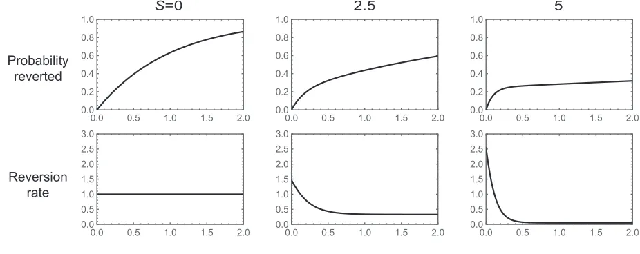
at the first site, so that the setA¼ fab;aBg and leavingA corresponds to ana/Asubstitution. Given that the popu-lation has already been evolving on thisfitness landscape for a long time and that ana/Asubstitution has just occurred, we want to understand the distribution of times until anA/ asubstitution occurs as a function of the depth of thefitness valleyS.
This distribution of times is easy to understand intuitively. ForSless than2 the dynamics are approximately neutral and the waiting time for reversion is approximately expo-nential with mean 1. For larger S, the dynamics are sub-stantially affected by the fitness valley. The best way to understand these dynamics is by considering where the pop-ulation is immediately after ana /Asubstitution. At sta-tionarity, we know that the frequency of substitutions into thefitness valley must be equal to the frequency of substitu-tions out of the valley. This means that at stationarity, half the time the population will have justfixed the valley geno-typeAband half the time it will havefixed the peak genotype AB:Populations thatfix the peak genotypeABare unlikely to revert in the short term, whereas populations that fix the valley genotype Abare likely to move to one or the other peak in the short term, with equal probability. Thus, roughly speaking, after a short time the population will either have reverted (with probability 1/4, since half the time itfixes the valley genotype and then immediately reverts half the time) or befixed at thefitness peakAB(with probability 3/4). This means that reversions happen either very shortly after the initial substitution—and this occurs 1/4 of the time—or only after the long waiting time needed for deleteriousfixations to occur.
Figure 1 shows these dynamics as a function ofS. The top row shows the probability that anA/areversion has oc-curred as a function of time and the bottom row shows the reversion rate,hðtÞ:The leftmost column shows the neutral case. The reversion rate is constant and the probability that a reversion has occurred by time t is given by 12e2t: The center and right columns show the case where S¼2:5 and S¼5;respectively. In both cases, the reversion rate is high initially, starting at S=2 (probability 1/2 of starting at the valley genotype in which case returns toAoccur at roughly rateS). The reversion rate drops rapidly as populations leave the valley genotype, approaching an asymptotic rate of 3=2 the substitution rate of a deleterious fixation 2S=ð12eSÞ (populations that have not yet reverted are likely at theAB
fitness peak; reversion occurs either via a direct substitution ofaat rate2S=ð12eSÞor viafixation of the valley genotype Ab, which occurs at rate2S=ð12eSÞ;followed by reversion with probability 1/2). Thus, the reversion rate is initially high but rapidly approaches a much lower rate, which results in a characteristic“knee”in the probability that a population has reverted by timet, where a population has a substantial prob-ability of having reverted at short times (corresponding to a steep initial increase in the fraction reverted as a function of time), but populations that do not revert during this initial period have much lower reversion rates (resulting in a slow
increase in the fraction reverted after this initial period); see Figure 1, top row and center and right columns.
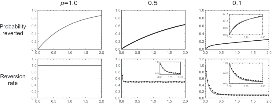
Mutational robustness and the rate of reversion: As a second example, we consider a biallelicfitness landscape with one focal site andLother sites, where each genotype is viable with probabilitypand all viable genotypes are neutral rela-tive to each other. All sites experience forward and reverse mutations at rate 1. This example is motivated by the model used by Kondrashov and colleagues to study long-term puri-fying selection (Breenet al.2012; Usmanovaet al.2015). We want to understand the dynamics of reversion at the focal site.
We proceed with a heuristic treatment based on the as-sumption thatLp1:In this regime, we treat each genotype as having a constant numberLpof neutral neighbors acces-sible by mutations at nonfocal sites. The key idea is that immediately after a substitution at the focal site, the back substitution is viable and so reversions initially occur at rate 1. However, once an additional substitution at a nonfocal site accrues, the probability that the reversion mutation at the focal site is viable is onlyp. Thus, the reversion rate drops very rapidly from 1 top.
In particular, after a substitution at the focal site, the expected substitution rate is 1þLpand the probability that thefirst substitution is a reversion is 1=ð1þLpÞ:Thus, we can approximate the probability distribution of waiting times un-til reversion as a mixture of two exponential distributions. Thefirst distribution has rate 1 and is weighted by the prob-ability that the population reverts before any other substitu-tion occurs, 1=ð1þLpÞ:The second exponential distribution has ratepand is weighted by the probability that a population experiences a substitution at another site before the reversion event occurs,Lp=ð1þLpÞ:This suggests that the probability of having reverted by timetcan be approximated by
FðtÞ 12 1 1þLpe
2ð1þLpÞ t2 Lp
1þLpe
2t: (16)
Based on a similar argument, we can approximate the re-version rate as
hðtÞ e2ð1þLpÞ tþp12e2ð1þLpÞ t; (17)
where thefirst term corresponds to the initial reversion rate of 1, which applies with probabilitye2ð1þLpÞ t(the probability of not having yet having experienced thefirst substitution), and the second term corresponds to the expected reversion rate given that one substitution has occurred,p, weighted by the probability that a substitution has already occurred, 12e2ð1þLpÞ t:
Although an exact treatment of any particular realization of the model is possible using the associated rate matrixQfull;the
a viable genotype and have just come from a viable genotype that differs only at the focal site. We simulated the subse-quent evolution of such a population under weak mutation, keeping track of the genotypes produced by mutation and whether they are viable (with probabilityp) or inviable (with probability 12p) until thefirst reversion event at the focal site. For each choice of parameters, we repeated this proce-dure 1,000,000 times.
The resulting reversion times are shown in Figure 2 for L¼100: The top row shows the probability of having reverted by timet, and the bottom row shows the reversion rate as a function of time. The left column shows the exact theoretical results for the case where all genotypes are viable (shaded lines). The center and right columns show the results for p¼0:5 andp¼0:1;respectively, with the approximate theoretical results given by Equations 16 and 17 shown as shaded lines and the simulation results shown as solid lines. For the casep¼0:5 the reversion rate drops rapidly from 1 to
p. Indeed, this drop is so rapid that relatively few popula-tions actually revert at the higher initial rate, which is as we expect, since the probability that a population reverts before experiencing another substitution is only
1=ð1þ10030:5Þ 0:02:On the other hand, for the case p¼0:1 we see a modest knee in the time evolution of the fraction of populations that have reverted. This is because a larger fraction 1=ð1þ10030:1Þ 0:09 of populations revert before experiencing another substitution, and the sub-sequent substitution rate is lower,0.1 instead of 0.5.
Intuitively, the knee shape illustrated in Figure 2 for small pand largeLparises because for smallpthere are fewer other loci at which a substitution can occur, and so populations stay at the genotype they initially arrived at—with its elevated reversion rate—longer, which leads to a substantial probabil-ity of having reverted at short times. However, eventually
such populations leave the initial genotype, at which time they experience lower reversions rates, p:This produces a pattern where the probability of having reverted becomes substantial at short times but thereafter grows very slowly. Although the theory is complicated and so we do not discuss it in detail here, it is worth noting that whenpis small enough thatLpbecomes small the waiting time until reversion again becomes short. Intuitively, this occurs because for very small Lpthe only viable mutation after a substitution at the focal site is the back mutation at the focal site, and thus essentially all reversions occur at the initial elevated rate.
More generally, this simple model suggests that the dy-namics of reversion should depend on the degree of muta-tional robustness even whenfitness is allowed to take more than two values. The key insight is that just after a substitution at a focal site, the population is not at a random genotype, but rather at one where the back substitution rate is likely to be unusually high. Now, if there is a high degree of mutational robustness, then the neutral substitution rate is high, and the population will leave this special genetic background quickly (cf. McCandlish 2013), so that when most reversions occur, the substitution rate for the back mutation is much lower than it was initially. When the degree of mutational robust-ness is very low, by contrast, the population will often stay at the initial genotype until the reversion occurs by a direct back substitution, which occurs at the initial rate. When the degree of mutational robustness is intermediate, we see a combina-tion of these two dynamics: a substantial fraccombina-tion of popula-tions revert via the direct back substitution from the initial genotype, and another substantial fraction revert at the lower rates that are typical of other genetic backgrounds. This in-termediate degree of robustness thus produces a characteris-tic knee in the time evolution of the probability that the population has reverted.
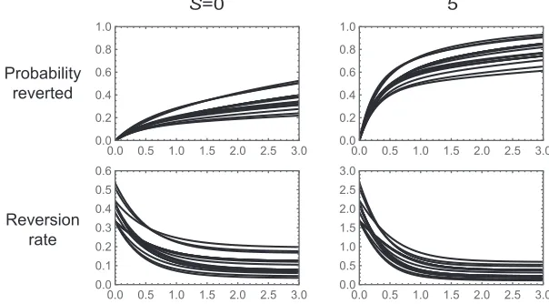
Amino acid reversion in codon models:The two examples we have considered so far describe the dynamics of reversion at a single site in a biallelic fitness landscape. For ourfinal example we consider the dynamics of a single amino acid under a codon model. Stop codons are treated as inviable, and mutations occur at each site with equal probability to each of the three alternative nucleotides (Jukes and Cantor 1969) with a total rate of 1 so that time is measured in the expected number of substitutions per synonymous site (Ks). We
imple-ment selection by assuming that genotypes with the focal amino acid are neutral relative to each other and have a scaled selective advantageSover all other amino acids.
Figure 3 shows the dynamics of reversion under this model for the neutral case,S¼0;and also for the case where the focal amino acid has a moderate selective advantage, S¼5 (each amino acid corresponds to one line; the fraction reverted is shown in the first row andhðtÞ is shown in the second row). The key insight for understanding these dynam-ics is that, just after a population leaves the set of codons that code for the focal amino acid, it can still mutate back to the focal amino acid. However, after additional substitutions ac-crue, the population is likely to be at a genotype that is no longer mutationally adjacent to the focal amino acid, leading to a decreasing reversion rate over time. In particular, for bothS¼0 andS¼5;the reversion rate drops from its initial value to nearly its asymptotic value byKs¼1:In the case of
S¼5;this produces a pronounced knee in the shape of the curve describing the time evolution of the probability that a population has reverted: more than one-third of populations are expected to revert almost immediately, whereas the remaining populations take a long time before they eventu-ally revert.
Discussion
We have analyzed reversions in a population that has just left some focal set of genotypesA. Our main interest has been the rate at which the populationfirst returns to the setA—that is, the rate at which the population experiences a reversion— and how this rate changes over time. For a population that has already been evolving on a constantfitness landscape for a very long time, we have shown that the rate of reversion to Ais nonincreasing in time. Furthermore, when the setA con-sists of all genotypes with a particular allele at a focal site in a biallelicfitness landscape, we have shown that the reversion rate is strictly decreasing if and only if epistasis is present at the focal site. We explored some simple examples of these reversion dynamics, to gain intuition about their magnitude and evolutionary impact.
We have also analyzed the case of a population that has been evolving on thefitness landscape only for a short time and whose initial state is therefore not drawn from the stationary distribution of the evolutionary dynamics. In this case we have shown that the time evolution of the reversion rate is, after a change in sign, mathematically identical to the time evolution of the mean Malthusianfitness for an infinite population evolving on an alteredfitness landscape where the substitution rates of the originalfitness landscape play the role of mutation rates and the rates of returns toAplay the role of genotype-specific death rates.
One consequence of reversion rates that decrease in time is a distinctive pattern, whereby a population either reverts very quickly after the initial substitution with some moderate probability or else takes a very long time to revert. If we consider the probability of having reverted plotted as a
function of time, such a pattern can be seen as a “knee”, where this curve rises rapidly at short times until the prob-ability of having reverted is substantial and then shifts to rising much more slowly. This pattern occurs because the expected rate of substitutions back to A at stationarity is particularly high if we condition on just having left A. As time passes and other substitutions accrue, the features of the genetic background that resulted in the unusually high substitution rate toAare lost. One consequence of this knee-like phenomenon is that the mean waiting time until rever-sion may not be very informative about the actual dynamics of reversion.
Our results show that at stationarity, a strictly decreasing reversion rate occurs whenever there is genotype-to-genotype variation in the rate of substitutions to the setA. When the set Acorresponds to the set of genotypes with a particular allele at a particular site, the presence of an epistatic interaction between the focal site and at least one other site is sufficient to produce such genotype-specific variation and hence suffi -cient for the reversion rate to be strictly decreasing. However, other factors besides epistasis can also be responsible for genotype-to-genotype variation in the rate of substitutions
to A. For instance, in our codon example, which has more
than two alleles per site, the structure of the genetic code itself results in variation in the substitution rate to any par-ticular amino acid, because the focal amino acid will not be mutationally accessible from all other codons. More gener-ally, the genotype–phenotype map will tend to produce genotype-to-genotype variation in the rate at which the focal phenotype becomesfixed in the population, so that the re-version rate for phenotypes should typically be decreasing. Finally, it is worth mentioning that while we define a site at the genotypic level by the feature that its mutational dynamics are independent of the states of the other sites, context-dependent mutation could also produce genotype-to-genotype variation in rates of substitution toA, which would again be sufficient for decreasing reversion rates (provided the result-ing Markov chain is still reversible).
It is also interesting to ask the converse question: What conditions could possibly produce reversion rates that in-crease in time? To do this, it is helpful to consider a way of restating our main result: if evolution can be modeled as a reversible Markov chain on the set of genotypes, then at stationarity the reversion rate to any subset of genotypes is nonincreasing with the time since the population left that subset. A reversible Markov chain is a Markov chain such that the probability of moving through any cycle of states in one direction is equal to the probability of moving around that cycle in the reverse direction (this is known as Kolmogorov’s criterion; see,e.g., Kelly 1979, section 1.5). Thus, a reversible Markov chain is simply a Markov chain with no cyclic biases. This means we can restate our main result as saying that reversion rates can increase in time, starting from stationar-ity, only if some factor induces a cyclic bias in the Markov chain describing evolution among genotypes.
It is known that, under weak mutation, adding frequency-and time-independent natural selection does not add any cyclic bias if no such bias is present in the mutational dynamics (i.e., the weak mutation Markov chain under constant frequency-independent selection is reversible if the muta-tional dynamics are reversible; see, e.g., Sella and Hirsh 2005). However, we may expect reversion rates to sometimes increase in time under conditions wherefitness is nontransi-tive (e.g., Kerret al.2002) or when environments change in a cyclic manner (e.g., Leslie et al.2004; Hensleyet al.2009; Berglandet al.2014). Under these types of conditions, natu-ral selection tends to push populations through a cycle of genotypic states in a periodic manner, which means that re-version becomes more likely as time passes.
Another condition that might produce increasing reversion rates is when the evolutionary dynamics are not stationary, for instance at the beginning of an adaptive transient. We have provided intuition for such circumstances by noting that, under time- and frequency-independent selection, the time evolution of the reversion rate can be recast as the time evolution of the mean fitness of an infinite population on
an alternativefitness landscape. This intuition suggests that the reversion rate should tend to go down just as the mean
fitness tends to go up, unless the infinite population starts at an unusually highfitness or the reversion rate starts at an un-usually low value. In the case of an adaptive transient, early adaptive substitutions will tend to be strongly favored by natural selection, meaning that the initial reversion rate is unusually low. In these circumstances we may expect the reversion rate to increase, particularly in the case of diminishing-returns epistasis, where mutations that have strong positive effects early in adaptation have much smaller effects toward the end of adaption (Draghi and Plotkin 2013; Kryazhimskiy et al. 2014; cf. Hartl et al. 1985; Hartl and Taubes 1996).
Our results help bring clarity to a recent controversy con-cerning site-specific amino acid preferences during protein evolution (Naumenko et al. 2012; Pollock et al. 2012; Ashenberget al.2013; Pollock and Goldstein 2014; Bazykin 2015; Doud et al. 2015; Goldsteinet al.2015; Risso et al. 2015; Shah et al. 2015; Usmanova et al. 2015). First, our results show that in the presence of epistasis, reversion rates will be decreasing in time and that the longer a population has left a set of genotypic states, the longer the expected time until reversion. However, our results show that when consid-ering reversion to an amino acid state, these results already hold even if there is no epistasis at the amino acid level, because of the structure of the genetic code itself. Indeed, it is worth noting that the epistasis already present in the ge-netic code is sufficient to produce many of the dynamical signatures of epistatic evolution even iffitnesses are additive at the amino acid level. For instance, it is easy to specify site-specific amino acid preferences that produce multipeaked
fitness landscapes at individual codons; such codons can have extremely long equilibration times, contrary to the analyses of Kondrashov et al. (2010) and Breen et al.(2013) who consider only the case where every amino acid can mutate to every other amino acid. Overall, decreasing reversion rates are a generic feature of evolution under long-term purifying selection and not a definitive signature of epistasis at the amino acid level.
Second, it is helpful to distinguish between what is expected when we consider a population that is conditioned to remain outside a subset of states vs. one that is simply restricted from entering that subset (cf. Ashenberg et al. 2013; Pollock and Goldstein 2014). The difference is whether, after a substitution, one considers only populations that have not yet reverted or whether all populations are prevented from reverting (but where we nonetheless keep track of the average propensity to return to the focal subset if such substitutions were to be permitted). We have shown that these two processes have different, but related, math-ematical characteristics. If there is any variation in the genotype-specific rates of return to the focal subset, then the reversion rate will be strictly decreasing for both process-es. While acclimatization of the rest of the genome to being in a new region of thefitness landscape contributes to
decreas-ing reversion rate for both processes, for the conditioned pro-cess there is also a statistical effect because populations that spend more time at genotypes with a rapid rate of return to the focal subset are likely to revert quickly. In addition, there is a simple mathematical relationship between these two processes: the asymptotic rate of transitions back to the focal subset when populations are restricted from entering it is the rate of an exponential distribution with mean equal to the expected reversion time, and this rate is bounded between the initial reversion rate and the asymptotic reversion rate when conditioning. Thus, while Ashenberget al.(2013) have criticized simulations where reversions are prevented from occurring as being unrealistic and misleading, such simula-tions are in fact more relevant to understanding the evolu-tionary process than would appear atfirst glance.
Finally, our results help clarify the relationship between various quantities observed in the literature and the entrench-ment phenomenon described here. Observed changes in site-specific amino acid preferences (Bazykin 2015) detected either by direct measurement (Doudet al.2015) or through comparative sequence analysis (Naumenko et al.2012) are sufficient to produce reversion rates that decrease in time under the assumption that sequence evolution occurs as a stationary reversible Markov chain. Furthermore, the nonlin-ear mapping between protein stability andfitness means that even if the stability effects of amino acid substitutions are more or less conserved (Rissoet al.2015),fitness effects will often be background dependent (Ashenberg et al. 2013), which is again sufficient to produce reversion rates that decrease in time. Fits of covarion-like models (Fitch and Markowitz 1970; Galtier 2001; Penny et al. 2001; Usmanova et al.2015) also suggest that rates of reversion should be decreasing in time, although as emphasized above the same qualitative effect can occur simply due to the struc-ture of the genetic code (Figure 3). It is also natural to ask about the predictions of the theory developed here for quan-tities observed in nature. Our predictions for the expected change in the selection coefficient of reversion are relatively weak. This is because the dynamics of the reversion rate and the dynamics of the expected selection coefficient of a rever-sion mutation may have qualitatively different shapes as a result of the nonlinearity in the probability of fixation and genotype-to-genotype variation in mutation rates. None-theless, it is the substitution rate that is most closely related to the evolutionary dynamics. This is why we can derive strong results on the reversion rate, but not on the time evo-lution of the average selection coefficient of reversions.
involve the Markov chain leaving and then reentering a focal subset as we look along the branches of the phylogeny. How-ever, more work is needed to extend our results to a phylo-genetic setting. This is because the distribution of waiting times observed on a phylogeny is different from the distribu-tion considered here where we condidistribu-tion on a substitudistribu-tion having just occurred. In addition, there are a variety of prac-tical problems with inferring substitution histories such as apparent homoplastic substitutions due to incomplete line-age sorting (Mendes and Hahn 2016) and the fact that sub-stitution histories are typically inferred using site-independent models even when there is substantial evidence for epistasis (e.g., Goldsteinet al.2015). Nonetheless, multiple studies in this broader literature (Rogozinet al.2008; Naumenkoet al. 2012; Soylemez and Kondrashov 2012; Goldsteinet al.2015; Zou and Zhang 2015) support our qualitative prediction that reversions and parallel substitutions should occur either very rapidly or only after a long waiting time.
Acknowledgments
We thank A. S. Kondrashov and an anonymous reviewer for their sage and helpful comments on the manuscript. This work was funded by the Burroughs Wellcome Fund, the David and Lucile Packard Foundation, U.S. Department of the Interior grant D12AP00025, National Institutes of Health training grant 2T32AI055400-11, and U.S. Army Research Office grant W911NF-12-1-0552.
Literature Cited
Aldous, D., and J. A. Fill, 2002 Reversible Markov chains and
ran-dom walks on graphs. Available at: http://www.stat.berkeley.
edu/aldous/RWG/book.html.
Ashenberg, O., L. I. Gong, and J. D. Bloom, 2013 Mutational
effects on stability are largely conserved during protein
evolu-tion. Proc. Natl. Acad. Sci. USA 110: 21071–21076.
Bazykin, G. A., 2015 Changing preferences: deformation of single
position amino acidfitness landscapes and evolution of proteins.
Biol. Lett. 11: 20150315.
Bergland, A. O., E. L. Behrman, K. R. O’Brien, P. S. Schmidt, and D.
A. Petrov, 2014 Genomic evidence of rapid and stable adaptive
oscillations over seasonal time scales in Drosophila. PLoS Genet. 10: e1004775.
Breen, M. S., C. Kemena, P. K. Vlasov, C. Notredame, and F. A.
Kondrashov, 2012 Epistasis as the primary factor in molecular
evolution. Nature 490: 535–538.
Breen, M. S., C. Kemena, P. K. Vlasov, C. Notredame, and F. A.
Kondrashov, 2013 Breenet al.reply. Nature 497: E2–E3.
Bridgham, J. T., E. A. Ortlund, and J. W. Thornton, 2009 An
epistatic ratchet constrains the direction of glucocorticoid
recep-tor evolution. Nature 461: 515–519.
Carneiro, M., and D. L. Hartl, 2010 Adaptive landscapes and
pro-tein evolution. Proc. Natl. Acad. Sci. USA 107: 1747–1751.
Collin, R., and M. P. Miglietta, 2008 Reversing opinions on Dollo’s
Law. Trends Ecol. Evol. 23: 602–609.
Conrad, M., 1990 The geometry of evolution. Biosystems 24: 61–
81.
Dollo, L., 1893 The laws of evolution. Bull. Soc. Bel. Geol.
Pale-ontol 7: 164–166.
Doud, M. B., O. Ashenberg, and J. D. Bloom, 2015 Site-specific
amino acid preferences are mostly conserved in two closely
re-lated protein homologs. Mol. Biol. Evol. 33: 2944–2960.
Draghi, J. A., and J. B. Plotkin, 2013 Selection biases the
preva-lence and type of epistasis along adaptive trajectories. Evolution
67: 3120–3131.
Fisher, R. A., 1930 The Genetical Theory of Natural Selection.
Clar-endon Press, London.
Fitch, W. M., and E. Markowitz, 1970 An improved method for
determining codon variability in a gene and its application to
the rate offixation of mutations in evolution. Biochem. Genet. 4:
579–593.
Galtier, N., 2001 Maximum-likelihood phylogenetic analysis
un-der a covarion-like model. Mol. Biol. Evol. 18: 866–873.
Gavrilets, S., 1997 Evolution and speciation on holey adaptive
landscapes. Trends Ecol. Evol. 12: 307–312.
Goldstein, R. A., S. T. Pollard, S. D. Shah, and D. D. Pollock,
2015 Nonadaptive amino acid convergence rates decrease
over time. Mol. Biol. Evol. 32: 1373–1381.
Gould, S. J., 1970 Dollo on Dollo’s law: irreversibility and the
status of evolutionary laws. J. Hist. Biol. 3: 189–212.
Grimmett, G., and D. Stirzaker, 2001 Probability and Random
Processes. Oxford University Press, London/New York/Oxford.
Hartl, D. L., and C. H. Taubes, 1996 Compensatory nearly neutral
mutations: selection without adaptation. J. Theor. Biol. 182:
303–309.
Hartl, D. L., D. E. Dykhuizen, and A. M. Dean, 1985 Limits of
adaptation: the evolution of selective neutrality. Genetics 111:
655–674.
Hensley, S. E., S. R. Das, A. L. Bailey, L. M. Schmidt, H. D. Hickman
et al., 2009 Hemagglutinin receptor binding avidity drives
in-fluenza a virus antigenic drift. Science 326: 734–736.
Iwasa, Y., 1988 Freefitness that always increases in evolution.
J. Theor. Biol. 135: 265–281.
Jukes, T. H., and C. R. Cantor, 1969 Evolution of protein
mole-cules, pp. 21–132 in Mammalian Protein Metabolism, Vol. 3,
edited by H. N. Munro. Academic Press, New York.
Kelly, F. P., 1979 Reversibility and Stochastic Networks(Series in
Probability and Mathematical Statistics). Wiley, Chichester, UK. Kerr, B., M. A. Riley, M. W. Feldman, and B. J. Bohannan,
2002 Local dispersal promotes biodiversity in a real-life game
of rock–paper–scissors. Nature 418: 171–174.
Kielson, J., 1979 Markov Chain Models—Rarity and Exponentiality
(Applied Mathematical Sciences, Vol. 28). Spring-Verlag, New York.
Kimura, M., 1983 The Neutral Theory of Molecular Evolution.
Cam-bridge University Press, CamCam-bridge, UK.
Kondrashov, D. A., and F. A. Kondrashov, 2015 Topological
fea-tures of rugged fitness landscapes in sequence space. Trends
Genet. 31: 24–33.
Kondrashov, A. S., I. S. Povolotskaya, D. N. Ivankov, and F. A.
Kondrashov, 2010 Rate of sequence divergence under constant
selection. Biol. Direct 5: 5.
Kryazhimskiy, S., D. P. Rice, E. R. Jerison, and M. M. Desai,
2014 Global epistasis makes adaptation predictable despite
sequence-level stochasticity. Science 344: 1519–1522.
Leslie, A., K. Pfafferott, P. Chetty, R. Draenert, M. Addo et al.,
2004 HIV evolution: CTL escape mutation and reversion after
transmission. Nat. Med. 10: 282–289.
McCandlish, D. M., 2013 On thefindability of genotypes.
Evolu-tion 67: 2592–2603.
McCandlish, D. M., and A. Stoltzfus, 2014 Modeling evolution
using the probability of fixation: history and implications. Q.
Rev. Biol. 89: 225–252.
McCandlish, D. M., E. Rajon, P. Shah, Y. Ding, and J. B. Plotkin,
2013 The role of epistasis in protein evolution. Nature 497:
McCandlish, D. M., C. L. Epstein, and J. B. Plotkin, 2015a Formal
properties of the probability offixation: identities, inequalities
and approximations. Theor. Popul. Biol. 99: 98–113.
McCandlish, D. M., J. Otwinowski, and J. B. Plotkin, 2015b Detecting
epistasis from an ensemble of adapting populations. Evolution 69:
2359–2370.
Mendes, F. K., and M. W. Hahn, 2016 Gene tree discordance
causes apparent substitution rate variation. Syst. Biol. DOI: 10.1093/sysbio/syw018.
Muller, H. J., 1918 Genetic variability, twin hybrids and constant
hybrids, in a case of balanced lethal factors. Genetics 3: 422.
Muller, H. J., 1939 Reversibility in evolution considered from the
standpoint of genetics. Biol. Rev. Camb. Philos. Soc. 14: 261–
280.
Naumenko, S. A., A. S. Kondrashov, and G. A. Bazykin, 2012 Fitness
conferred by replaced amino acids declines with time. Biol. Lett.
8: 825–828.
Penny, D., B. J. McComish, M. A. Charleston, and M. D. Hendy,
2001 Mathematical elegance with biochemical realism: the
covarion model of molecular evolution. J. Mol. Evol. 53: 711–
723.
Pollock, D. D., and R. A. Goldstein, 2014 Strong evidence for
protein epistasis, weak evidence against it. Proc. Natl. Acad. Sci. USA 111: E1450.
Pollock, D. D., G. Thiltgen, and R. A. Goldstein, 2012 Amino acid
coevolution induces an evolutionary Stokes shift. Proc. Natl.
Acad. Sci. USA 109: E1352–E1359.
Porter, M. L., and K. A. Crandall, 2003 Lost along the way: the
significance of evolution in reverse. Trends Ecol. Evol. 18: 541–
547.
Povolotskaya, I. S., and F. A. Kondrashov, 2010 Sequence space
and the ongoing expansion of the protein universe. Nature 465:
922–926.
Risso, V. A., F. Manssour-Triedo, A. Delgado-Delgado, R. Arco, A.
Barroso-delJesus et al., 2015 Mutational studies on
resur-rected ancestral proteins reveal conservation of site-specific
amino acid preferences throughout evolutionary history. Mol.
Biol. Evol. 32: 440–455.
Rogozin, I. B., K. Thomson, M. Csürös, L. Carmel, and E. V. Koonin,
2008 Homoplasy in genome-wide analysis of rare amino acid
replacements: the molecular-evolutionary basis for Vavilov’s law
of homologous series. Biol. Direct 3: 7.
Rokas, A., and S. B. Carroll, 2008 Frequent and widespread
par-allel evolution of protein sequences. Mol. Biol. Evol. 25: 1943–
1953.
Sella, G., and A. E. Hirsh, 2005 The application of statistical
phys-ics to evolutionary biology. Proc. Natl. Acad. Sci. USA 102:
9541–9546.
Shah, P., D. M. McCandlish, and J. B. Plotkin, 2015 Contingency
and entrenchment in protein evolution under purifying
selec-tion. Proc. Natl. Acad. Sci. USA 112: E3226–E3235.
Simpson, G. G., 1953 The Major Features Of Evolution. Columbia
University Press, New York.
Soylemez, O., and F. A. Kondrashov, 2012 Estimating the rate of
irreversibility in protein evolution. Genome Biol. Evol. 4: 1213–
1222.
Tan, L., S. Serene, H. X. Chao, and J. Gore, 2011 Hidden
random-ness betweenfitness landscapes limits reverse evolution. Phys.
Rev. Lett. 106: 198102.
Teotónio, H., and M. R. Rose, 2001 Perspective: reverse
evolu-tion. Evolution 55: 653–660.
Usmanova, D. R., L. Ferretti, I. S. Povolotskaya, P. K. Vlasov, and F.
A. Kondrashov, 2015 A model of substitution trajectories in
sequence space and long-term protein evolution. Mol. Biol. Evol.
32: 542–554.
Vaupel, J. W., and A. I. Yashin, 1985 Heterogeneity’s ruses: some
surprising effects of selection on population dynamics. Am. Stat.
39: 176–185.
Zou, Z., and J. Zhang, 2015 Are convergent and parallel amino
acid substitutions in protein evolution more prevalent than
neu-tral expectations? Mol. Biol. Evol. 32: 2085–2096.
Appendix A: The Distribution of Reversion Times at Stationarity
Our analysis of the distribution of reversion times at stationarity relies on the fact that the matrixQ;which gives the rates for the absorbing Markov chain describing the evolution dynamics until the time of reversion, admits an eigendecomposition. We develop this eigendecomposition and its properties and then use these results to show that the distribution of reversion times at stationarity can be expressed as a mixture of exponential distributions. We then use a very similar analysis to understand the modified process where reversion events are not permitted to occur.
We derive the eigendecomposition ofQbyfirst noting some features of the larger matrixQfull:Because the Markov chain
defined byQfullis reversible, it satisfies the detailed balance relationpfullðiÞQfullði;jÞ ¼pfullðjÞQfullðj;iÞfor alli;j:As a
conse-quence, the matrixD1=2
pfullQfullD
21=2
pfull is symmetric, whereDydenotes the diagonal matrix with the vectoryas its main diagonal. Now, define the vectorpof lengthn¼ jAcjsuch thatpðiÞ ¼p
fullðiÞ=
P
j2AcpfullðjÞfori¼1;. . .;n:The matrixD1p=2QD2p1=2is
thus symmetric, since it is simply a constant times a diagonal block of the symmetric matrixD1=2
pfullQfullD
21=2
pfull :We can thus expandD1=2
p QD2p1=2 in terms of its eigenvalues and eigenvectors as
2D1=2
p QD2p1=2¼
Xn
k¼1
lkukuTk; (A1)
where 0,l1#l2#l3#. . .#lnare the eigenvalues of2D1p=2QD2p1=2and the eigenvectorsukare orthonormal (the eigen-values are real because 2D1p=2QDp21=2 is symmetric and negative because they are same as those of 2Q;whereQis the generator of an absorbing Markov chain so that all of its eigenvalues have negative real parts).
We can now use this decomposition of2D1=2
p QD2p1=2 to likewise decomposeQ:In particular, multiplying Equation A1 by D21=2
p from the left andD1p=2from the right gives us
2Q¼X
n
k¼1 lk rk lT
k; (A2)
wherelk¼D1p=2ukandrk¼D2p1=2ukare the left and right eigenvectors of2Qassociated withlk:
Using this decomposition, we can then write the probability density function of the distribution of reversion times at stationarity as
fðtÞ ¼xTtg (A3)
¼xT
0e
Qtg
(A4)
¼xT
0
Xn
k¼1
e2lkt rk lTk
!
g (A5)
¼ 1
pTg g TD
p
Xn
k¼1
e2lkt rk lTk
!
g (A6)
¼ 1
pTg
Xn
k¼1 e2lkt
lT
kg
2
; (A7)
where we have used the fact that at stationarityx0ðiÞ}pðiÞgðiÞ(Equation 7). Thus,fðtÞis a mixture of exponential densities
with ratesl1;. . .;lnwhere the exponential density with ratelkhas weightðlTkgÞ
2=ðl
k pTgÞ:
We just showed that the distribution of reversion times at stationarity is afinite mixture of exponential distributions. We now show that the hazard function for anyfinite mixture of exponential distributions is nonincreasing. In particular, iffðtÞis afinite mixture of exponential densities
fðtÞ ¼X
m
witham;um.0; X
mam¼1;then the hazard function is
fðtÞ FðtÞ¼
X
mamume 2umt
X
mame2u
mt : (A9)
Differentiating the hazard function, we see that that the sign of the derivative depends only on the sign of
FðtÞf9ðtÞ2F9ðtÞfðtÞ ¼FðtÞf9ðtÞ þ ðfðtÞÞ2 (A10)
¼ 2X
i;j
aiaju2j e2ðuiþujÞtþ
X
i;j
aiajuiuj e2ðuiþujÞt (A11)
¼ 2
0
@ X
i;j with i6¼j
aiaj e2ðuiþujÞt
u2
j 2uiuj
1A
(A12)
¼ 2
0
@ X
i;j with i.j
aiaj e2ðuiþujÞt
u2
j 22uiujþu2i
1A
(A13)
¼ 2
0
@ X
i;j with i.j
aiaj e2ðuiþujÞtðui2ujÞ2
1
A; (A14)
which is nonpositive since each term in the sum is a product of nonnegative quantities and hence nonnegative. Thus, the hazard function is nonincreasing.
We turn now to the analysis of the modified process with rate matrixQ*¼QþDg;whereDgis the diagonal matrix withgon its main diagonal. Let us start by assuming thatAc is mutationally connected; we will return to the case of disconnectedAc
momentarily. First, note thatQ * differs fromQonly on its diagonal entries. Thus, following our analysis forQ;Dp1=2Q *D2p1=2is symmetric and can be expanded in terms of its eigenvalues and eigenvectors as
2D1=2
p Q *D2p1=2¼
Xn
k¼1 l*
k u*ku*Tk ; (A15)
where 0¼l*
1,l*2#l*3#. . .#l*nare the eigenvalues of2Dp1=2Q *D2p1=2and the eigenvectorsu*kare orthonormal (we have 0¼l*
1,l*2 becauseA
c is connected and so the continuous-time Markov chain generated byQ * is ergodic). With this
de-composition in hand, we can writel*
k¼D
1=2
p u*kandr
*
k¼D2
1=2
p u*kas the left and right eigenvectors of2Q * associated withl
*
k and write the reversion rate under the modified process as
f *ðtÞ ¼xT0eQ*tg (A16)
¼xT
0
Xn
k¼1 e2l*kt r*
k l*Tk
!
g (A17)
¼ 1
pTgg TD
p
Xn
k¼1 e2l*kt r*
k l*Tk
!
g (A18)
¼pTgþ 1
pTg
Xn
k¼2 e2l*kt
l*T
k g
2
; (A19)
where we have used the fact that the row sums ofQ * are all 0 so thatr*
1is the vector of all 1’s and thusl*1¼Dpr*1¼p:Because
l*
k.0 fork$2;this expression is clearly strictly decreasing intunlessn¼1 (in which casegðiÞis obviously constant) orl
*T
k g= 0 fork$2:In the latter case, we haveu*T
k D
1=2