Flow Scheduling: An Efficient Scheduling Method for
MapReduce Framework in the Decoupled Architecture
Chin-Jung Hsu
Department of Computer Science North Carolina State University
[email protected]
Vincent W. Freeh
Department of Computer ScienceNorth Carolina State University
[email protected]
ABSTRACT
Hadoop is a popular implementation of the MapReduce pro-gramming model for data processing. We first compare dif-ferent Hadoop models and discuss their advantages and lim-itation. The traditional Hadoop system is scalable because a machine serves both computation and storage function. However, this principle imposes a strong constraint on sys-tem design and does not quite fit enterprise and cloud appli-cation, which require to decouple computation and storage nodes. Any naive Hadoop implementations may fail to be optimized because they are designed to preserve data local-ity, which does not exist in the decoupled model. In this paper, we propose a flow scheduling method: it eliminates undesired factors that can decrease processing performance. We model the cost of task assignment based on the penalty of violating flow demand and convert this problem to the network optimization problem. We have implemented Flow Scheduler for Hadoop and the experiment results show that it can maximize the processing flow rate while improving the system throughput by up to 30%. More interestingly, our flow scheduling method can provide more smooth task execution time, which suggests it can eliminate stragglers that caused by resource contention.
Categories and Subject Descriptors
D.4.1 [Operating Systems]: Process Management— schedul-ing; C.2.4 [Computer-Communication Networks]: Dis-tributed Systems—distributed applications; G.2.2 [Discrete Mathematics]: Graph Theory—graph algorithms, network problem
General Terms
Design, Algorithms, Performance
1.
INTRODUCTION
This is an era of big data, and IDC even estimated the exponential growth of data by a factor of 10 [21, 29]. The
Permission to make digital or hard copies of all or part of this work for personal or classroom use is granted without fee provided that copies are not made or distributed for profit or commercial advantage and that copies bear this notice and the full citation on the first page. To copy otherwise, to republish, to post on servers or to redistribute to lists, requires prior specific permission and/or a fee.
Copyright 20XX ACM X-XXXXX-XX-X/XX/XX ...$15.00.
0 1 2 3 4 5
WordCount Terasort Grep
Elapsed Time (Normalized)
Hadoop(EC2) Amazon Elastic MapReduce
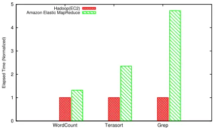
Figure 1: Hadoop performance in the decoupled model. Four x1.large instances are used, and Ama-zon EMR uses AmaAma-zon S3 as the storage for in-put and outin-put files. Amazon EMR does not utilize all available machines because its resource scheduler does not fit the decoupled Hadoop model.
growing data set provides huge potential for business and research to explore. Thus, big data analytics has become critical demand to dig valuable information from explosive growing data. The giant volume of data along with its va-riety and velocity poses great challenge to big data ana-lytics[35], and therefore its optimization remains an active research domain.
The MapReduce programming model has gained increas-ing success for parallel data processincreas-ing because of its hori-zontal scale and fault tolerance [13]. Apache Hadoop [4] and Microsoft Dryad [18], for example, are popular systems that embrace this model. In order to handle large-scale data, these systems usually run on top of large clusters of com-modity machines and tightly couple computation and stor-age nodes. This design enables a system to scale out easily because the ratio between computation power and I/O ca-pability remains constant [13, 4, 10].
stor-age, data lifecycle management and elastic cloud storage. More importantly, this separate architecture provides high flexibility of system deployment, which is a big challenge in enterprise and datacenter management [30, 27]. For these reasons, we believe the decoupled model will become more important for MapReduce and Hadoop.
The decoupled mode has emerged but only few research studies pay attention to this scenario. This situation leads to poor performance when running Hadoop with the decou-pled model as shown in Figure 1. To understand the perfor-mance of the decoupled model, we ran three different types of jobs on Amazon EC2 for the Hadoop reference model and Amazon Elastic MapReduce for the decoupled one. The re-sult shows that the decoupled model has system throughput that is much lower than we expected. We find that exist-ing Hadoop schedulers cannot work well when data locality no longer exists. Besides, we doubt that the overhead of large data movement can greatly affect system throughput because the storage system and the network infrastructure cannot fulfill the demand of Hadoop applications.
In this paper, we view the decoupled Hadoop model as a flow network in which data flows through computation and storage facilities. The data flow rate is the amount of data processed or transferred per unit of time, and the system throughput can be measured by the flow rate. We argue that maintaing high data flow rate can increase the system throughput. In the decoupled model, there are two possible conditions that a computation facility does not fully utilize its processing power: 1) the flow rate of data supply from the remote storage facility is not fast enough and 2) the com-puting facility cannot process data flow fast enough. The first case can happen when the storage facility cannot han-dle a large number of simultaneous data access and when network infrastructure cannot sustain such a large amount of data transfer, especially when cross-rack communication happens. The second case comes from the overhead of oper-ating system and the data access over network. We believe eliminating undesired factors that affects the processing flow rate can increase the system throughput in the meanwhile.
We propose a flow scheduling method that models the penalty cost of task assignments. Given the cost model, we encode the scheduling problem as the min-cost flow problem so that we can derive the optimal task assignment. We have designed Hadoop Flow Scheduler that implements our flow scheduling method. This Flow Scheduler requires job pro-file and machine propro-file in order to decide the optimal task assignment. We first estimate the flow demand of tasks and the flow capability of facilities and then feed this informa-tion to our Flow Scheduler. Our experiment result shows that we can improve the system throughput by up to 30%. More importantly, our flow scheduling method can eliminate stragglers in the decoupled model and provide more smooth task execution time.
This paper is organized as follows. Section 2 provides the background on the new Hadoop design and the decou-pled model. Section 3 describes the ideal behind our flow scheduling method, the definition of data flow rate and the cost model for task assignment. Section 4 details the Flow Scheduler implantation for Hadoop and how we estimate the data flow rate. We evaluate Flow Scheduler in Section 5 and discuss the limitation of current implementation. Section 6 gives the most related work and we conclude in Section 7.
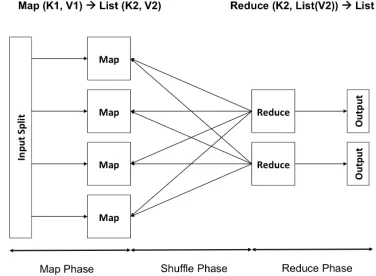
Figure 2: A MapReduce job consists of the map, shuffling and reduce phase. The map task processes a portion of input data and the reduce task aggre-gate the output from map tasks. The phase between the map and the reduce phase to dispatch interme-diate result is the shuffling phase.
2.
BACKGROUND
2.1
MapReduce Programming Model
The MapReduce programming model [13] is a simplified model for data processing. In the MapReduce model, a data processing job consists of three phases. First, the map phase processes a portion of input data and generates output as a list of key/value pairs. Next, the shuffle phase is the pe-riod to transfer data between map tasks and reduce tasks Finally, the reduce phase merges the output, which is aggre-gated by key, from the map phase. Many data processing applications can benefit from this simplified model, such as large-scale indexing, machine learning problems and graph computation [13]. Google and Yahoo, for example, apply this model to accelerate large-scale data processing and em-power their online advertisement business.
Figure 2 shows the three phases in a MapReduce job. This simplified model is relatively easy for programmers to de-velop a MapReduce application. Programmers only need to implement the map function and the reduce function. Each map function processes a portion of input data at a time, e.g. one line of a file or a XML document, and the output of the map function is a list of key-value pairs. The reduce function then aggregates those key-value pairs and generates the final output. Programmers do not need to specify the details of the shuffling phase. The MapReduce runtime han-dles complex data exchange: it aggregates the results based on the output key from the map phase, and then transfers the output to corresponding reduce tasks.
mecha-nism; it needs only re-run the failed task again. In short, the MapReduce programming is simple but yet powerful enough to achieve the goal of many practical data processing appli-cations.
2.2
Hadoop
Hadoop [4] is an open-source implementation of the MapRe-duce programming model, which provides a reliable and scal-able system for data processing. The latest Hadoop project includes four modules: 1) Hadoop YARN is a cluster re-source management framework, 2) Hadoop MapReduce is the implementation to support the MapReduce program-ming model based on YARN, 3) Hadoop HDFS is a dis-tributed storage system for Hadoop application data, and 4) Hadoop Common is the common utilities that are required by the above modules.
2.3
Hadoop Job Execution Flow
1
The Resource Manager (RM) is responsible for resource allocation. Once received a MapReduce job, RM allocates resource to initialize a AppMaster. This AppMaster is cre-ated to negotiate computing resources with the preconfig-ured resource scheduler, e.g. FIFO Schduler, Capacity Sched-uler [2], Fair SchedSched-uler [3]. These schedSched-ulers allocate re-sources (or slots) to the AppMaster based on objectives such as data locality or fairness. Those allocated resources can be used to run map or reduce tasks. Different from Hadoop 1.x (non YARN based Hadoop), the number of map and reduce slots is required to define explicitly, and research studies [9, 32] show that the optimal configuration of this value is not intuitive. The YARN resource framework, on the other hand, is flexible because it determines these numbers dy-namically based on the application request and the node capability.
After obtaining computation resources, the AppMaster starts several node containers to process input splits. Each map task handles an input split, and the size is usually 64MB or 128MB (the block size of HDFS). This input split is parsed by the RecordReader object and the map task processes a record at a time. Each record read operation creates the FSDataInputStream object to access the file in-put stream as shown in Figure 3. The source of the inin-put split can be a block from HDFS or it can an data object from Amazon S3 or Azure Blob Storage service.
2.4
Hadoop Models
The most common way to deploy a Hadoop system is to configure a node to run both Hadoop MapReduce and Hadoop HDFS, which can avoid bringing data to computa-tion. However, data management, in many cases, requires separating computing and storage nodes for flexibility and efficiency. For example, enterprises prefer silos in order to manage high-value data. Amazon Elastic MapReduce pri-mary uses Amazon S3 for its persistent data storage. More-over, many high performance files systems are considered to replace HDFS in order to support both MapReduce appli-cation and other workload. As a result, different scenarios require different ways to deploy Hadoop. As shown in Figure 3, we can define three major types of Hadoop configuration as follows.
1The latest YARN framework allocates resources based on
memory and CPU will be considered soon
Figure 3: System configuration of Hadoop. Each slot handles one input split and uses the Recor-dReader object to read data from a POSIX compli-ant file system or a non-POSIX complicompli-ant file sys-tem, e.g. distributed data store.
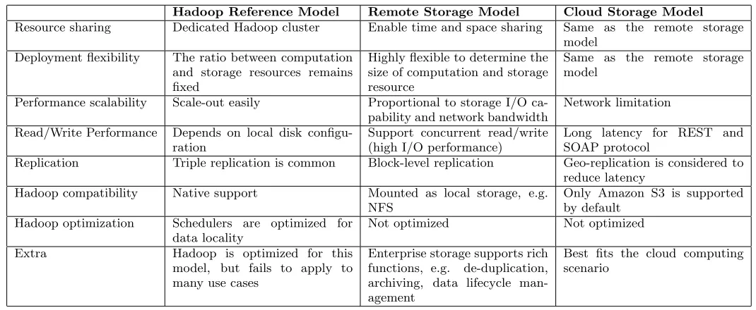
1. The reference model is the most common config-uration for dedicated Hadoop clusters. Each node in a Hadoop cluster serves both computing and storage functions. This model has the scale-out benefit be-cause the ratio between computation and storage re-mains constant. Each computation node own its own private storage (local disks), which can provide Hadoop jobs enough data access bandwidth. Most popular Hadoop schedulers aim to maximize the number of lo-cal map tasks so that data access is at lolo-cal but not from remote. This approach guarantees enough I/O bandwidth when the number of computation nodes increase. On the other hand, the output data of re-duce tasks will be written to the local HDFS (the data node), and then replicated to other remote data nodes.
2. Remote Storage Modelis common in enterprises or high performance computing (HPC). This model has the similar definition of AoE architecture [30]. NFS and SAN are quite common to store data, and Hadoop might require to access data in a separate storage, other than HDFS. In this case, each computation node can access data via file-level protocol or block-level protocol (mounted as a local file system). The mounted point should appear the same across all computation nodes, and thus data can be accessed on any nodes. An good example is to replace HDFS with GPFS [7].
Table 1: Comparisons of Hadoop models with different storage architecture
Hadoop Reference Model Remote Storage Model Cloud Storage Model
Resource sharing Dedicated Hadoop cluster Enable time and space sharing Same as the remote storage
model Deployment flexibility The ratio between computation
and storage resources remains fixed
Highly flexible to determine the size of computation and storage resource
Same as the remote storage model
Performance scalability Scale-out easily Proportional to storage I/O
ca-pability and network bandwidth
Network limitation
Read/Write Performance Depends on local disk configu-ration
Support concurrent read/write (high I/O performance)
Long latency for REST and SOAP protocol
Replication Triple replication is common Block-level replication Geo-replication is considered to
reduce latency
Hadoop compatibility Native support Mounted as local storage, e.g.
NFS
Only Amazon S3 is supported by default
Hadoop optimization Schedulers are optimized for data locality
Not optimized Not optimized
Extra Hadoop is optimized for this
model, but fails to apply to many use cases
Enterprise storage supports rich functions, e.g. de-duplication, archiving, data lifecycle man-agement
Best fits the cloud computing scenario
This configuration forces a task to read and write data from and to the remote storage service.
Contrary to the reference model, we classify the remote storage model and the cloud storage model as the decoupled model. Because the decoupled Hadoop model can provide more flexibility in deployment and thus the decoupled model would be our focus in this paper.
Different from traditional Hadoop model, data locality is no longer valid for scheduling jobs, which can cause exist-ing scheduler not suitable for the decouple Hadoop model. Moreover, the decoupled Hadoop model can face perfor-mance degradation because all the input data have to be transferred over the network In such a case, the system throughput can be affected because CPU can be idle while waiting for the data to be ready. For these reasons, the de-couple model requires a new scheduling algorithm for better performance.
In order to optimize the system throughput (minimizing turnaround time), we argue that maximizing the data pro-cessing rate on computing nodes can greatly increase the system throughput. The data processing rate can be af-fected if the input data cannot be pulled quickly enough or the output data cannot be pushed to remote storage nodes. To address this challenge, we introduce flow scheduling in the next.
3.
FLOW SCHEDULING
In this section, we describe the concept of flow scheduling and then explain how we model the assignment cost based on the penalty of violating flow demand. We also introduce how to encode the scheduling problem as a min-cost flow problem.
3.1
Concept of Data Flow
A MapReduce job includes several map and reduce tasks, and each of them (on a computing facility) reads data, pro-cesses data and writes data. The data flow rate is the size of
data that goes through a facility per unit time. For exam-ple, the processing flow rate is how fast a machine can pro-cess data, and a faster propro-cessing rate also suggests higher system throughput. In a decoupled model, all of the read and write operations involve network activities, which can be costly and decrease the processing flow rate. Therefore, our flow scheduling tries to maximize processing flow rate on computing facilities so that the system throughput can be increased.
The idea of flow scheduling is similar to the water treat-ment system. Water supply to a desired end-user must go through several processing steps before water is delivered to users. Users may complain if water supply is not fast enough. This situation can happen if water supply is scarce or if the intermediate facilities cannot process water quickly or if the pipeline is not large enough or if too many users request water at the same time. Thus, to meet the demand from users, a water treatment system should satisfy the above conditions as mush as possible. This analogy truly reflects those factors that affect the system throughout in a decoupled Hadoop model: ensuring the quality of data supply and the flow rate of data processing can increase the system throughput. More precisely, if the flow demand of a task cannot be satisfied by facilities, the scheduling decision is considered costly.
Flow rate is defined as how fast a machine can process data or a network can transfer data.
R=D
T
Here,Dis the size of data andT is the total time to process or transfer the data. Throughput this paper, we usesecond for the time unit andmega bytesfor the data size unit.
facilities. The process flow capability is defined by how fast a facility can process data. Facilities can be classified as computing nodes, storage nodes and network infrastructure.
Rs
inis the read flow capability of the storage node andRsout
is the write one; similarly, Rnin and R n
out are for network
infrastructure, and the computing node usesRinc and Rcout
for read and write capability. Besides, only the computing node has the process flow capability,Rc
p.
Flow demand of tasks: The flow demand describes the characteristic of tasks and can be used to classify tasks into CPU-intensive (low flow demand) and network-intensive (high flow demand) tasks. A flow rate can vary during task execu-tion, and we assume the flow rate is relatively stable, which can be reasonable because either a map task or a reduce task repeats a piece of the same code based on key-value pairs. TheRtin and Rtout are the read and write flow demand of
tasks.
3.2
Cost Model
In this section, we describe how to model the cost of task assignment. The decoupled model can be model as{C, S, I}, where C is the set of computing facilities, S is the set of storage facilities and I is the network infrastructure. Let
ci ∈C, si ∈ S, wherei is an integer. The flow capability
of facilities is defined as, for example,Rci
p for the processing
capability on the computing nodeiand Rsi
out for the write
capability on the storage nodei. Letrc
p be the processing
flow rate on a computing facility. Whenrcpapproaches toRcp,
the system throughput is considered increasing. The tasks to be scheduled aretij, whereiis theith job in the system
andj is thejth task of the job. Similar to flow capability,
Rtij
in andR
tij
outare the read and write flow demand of tasks.
A scheduling problem is to assignT={tij}toC={cn},
and our flow scheduling tries to minimize the assignment cost based on the flow rate. Given a task, the cost of an assignment can be defined as the penalty cost that facilities cannot satisfy the flow demand of the task. To fulfill the flow demand of tasks, we should ensure quality flow supply and quality processing flow. There are two conditions in which an assignment can occur high penalty cost: 1) a storage facility is overloaded whenP
tij∈siR tij
in is high, especially
when it exceedsRsi
outand 2) a computing facility is filled with
network-intensive jobs, which meansP tij∈ciR
tij in is high.
To assign a map task tij, suppose the input data stores
onsn, the cost to assign the task oncnis the sum of
Rtij
in ×(1 +
rsn out
Rsnout
+fc)
and
Rtij
in ×(1 +em),
wherefc is the parameter if sn and cm is not in the same
rack, andem is the effective load oncm. The effective load
can be defined as P tij∈cmR
tij
in −stdev(R tij
in). If flow
de-mands of tasks are diverse on a computing facility, we con-sider the assignment cost lower because overlapping CPU-intensive and network-CPU-intensive tasks can utilize resource efficiently.
Whentijis a reduce task, it usually reads data from
mul-tiple computing facilities; thus, we need to count all of these read cost. Supposetijis assigned tocmand the reduce task
need to read data from other computing facilities ck, the
total read cost is
Figure 4: Flow scheduling uses the penalty cost to build the min-cost flow network. The number of supply means the number of tasks to be scheduled.
X
ck
Rtij
in ×(1 +
rck out
Rck out
+fc),
where fc has the definition similar to the one above. If
cm and ck are the same node, the parameter is zero, and
otherwise, the parameter is small for in-rack communication and large for cross-rack data transfer.
3.3
Min-cost flow optimization
We argued that maximizing the processing flow rate can increase the system throughput. As described in Section 3.2, we model the cost of task assignments as the penalty of vi-olating flow demand. Given the cost model, we encode the scheduling problem as a min-cost flow optimization prob-lem. The min-cost flow problem is a network optimization problem that looks for the cheapest way to allow a certain amount of flow through a network. Given the flow demand of map and reduce tasks, we can decide the best path of network flow with minimum penalty cost. For example, our flow scheduling avoids to assign a task to facilities if the flow capability of the facilities can not meet the flow demand of the tasks. Figure 4 depicts how to encode the scheduling problem to a min-cost flow problem.
The min-cost flow problem can be stated as follows:
M inimize z(x) = X
(i,j)∈A
cijxij
subject to
X
j:(i,j)∈A
xij− X
j:(j,i)∈A
xji=b(i)∀i∈N
0≤xij≤uij∀(i, j)∈A
In this equation,N={Tij, Ck, source, sink}and the source
node produces flow of capacity n, which is the number of available slots on computing facilities and the sink node has the flow of capability−n. Each arc fromTijtoCk has the
source toTij are bothone, and them of the arc fromCkto
the sink are the number of available slots onCk. After
en-coding the scheduling problem, we then solve the min-cost flow problem to decide the optimal task assignment.
4.
FLOW SCHEDULER FOR HADOOP
Hadoop supports pluggable resource schedulers that makes developing the flow scheduler not being a difficult challenge.
4.1
System Architecture
Our flow scheduler requires job profile (flow demand of tasks) and machine profile (flow capability of facilities). Be-sides, we use a database to keep track of resource allocation so that next time we can understand the flow rate on fa-cilities. The flow scheduler runs upon AppMaster requests resources or periodically, e.g. every 5 second. In each run, it calculate the penalty cost based on flow demand of tasks and flow capability of facilities, and then encodes the scheduling problem as stated in Section 3.3. After building the cost mode, we use the scaling push-relabled method as described in [15] and their solver program to derive the optimal task assignment.
4.2
Estimating Flow Rate
In this section, we describe how to estimate the flow de-mand of tasks and flow capability of facilities. Basically, we overload facilities to get flow capability and run a single task to derive the flow demand. First, we measureRc
outof storage
nodes to get the flow rate that a storage node can supply. We create a NoComputation map task that only reads input data, but does not do computation and does not generate output. We execute enough NoComputation map tasks at the same time to ensure that the out-bound bandwidth of a storage node is saturated. The result shows thatRcapout of
storage nodes is roughly close to 65% of the theoretical net-work bandwidth. Similarly,Rsin is close toR
s
out; therefore,
we use the same number. Regarding the flow capability of network infrastructure, we use the same number with that of storage nodes. This is true for node communication in the same rack; however, the cross-race communication can be limited by aggregate bandwidth available at top-of-rack switches. The real bandwidth of cross-bandwidth is hard to measure and monitor, and instead, we increase the cost of cross-rack communication in our cost model as described in 3.3.
For the flow capability of computing nodes,Rinc andRcout
are set to the same with storage nodes because this number is mainly limited by the network bandwidth. RegardingRc
p,
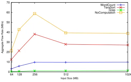
we ran different types of Hadoop jobs to estimate the pro-cessing capability of computing nodes. In order to faithfully measure the processing capability, we increased the number of map tasks while keeping only one reduce tasks running on the same node. As shown in Figure 5, the maximum flow capability happens when four maps are executed on a four-core node. Even with NoComputation jobs, the max
Rcpis around 60M B/s, which suggests the limitation of
net-work bandwidth and the overhead of Hadoop framenet-work af-fects the maximum flow rate of processing in the decoupled Hadoop model. Unless we can break these bottlenecks, we will not be able to increase the the flow rate of processing. Table 2 shows the flow capability that will be used later in our evaluation.
To estimate the flow demand of tasks, we vary input sizes
0 10 20 30 40 50 60 70
64 128 256 512 1024
Aggregate Flow Rate (MB/s)
Input Size (MB)
WordCount TeraSort Grep NoComputation
Figure 5: Estimating flow rate of processing capa-bility. Increasing the number of concurrent tasks does not necessarily increase the aggregate through-put; instead, it decreases the throughput, especially when the tasks are network intensive. The com-puting facility in Cluster 1 has the processing flow capability lower than 60MB/s in
to measureRtin for map tasks, and we fixed the number of
reduce tasks to one. We pick up the flow rate when only one map executes in a computing facility. This ensures that other tasks would not compete resources with the map task we measure. Routt of map tasks is set to zero because the
output data would be staged and later will be pulled by reduce tasks.
It is more tricky to estimateRtinof reduce tasks because
there are multiple sources of flow supply (the shuffle phase contains many-to-many communication [12]) and a reduce task can start even before all map tasks complete. Moreover, the input size can also affect the flow demand. These cases can make the elapse time of reduce tasks longer and would affect the accuracy of estimating flow demand. To eliminate the impact, we use only one reducer in our estimation and we calculate the real flow demand in runtime, which is described as in Section 3.3.
Table 2: Estimated flow capability of facilities. Clus-ter 1 is powerful than ClusClus-ter 2 and their detailed configurations are describe in Section 5
Facility Type Rpc Routs
Cluster 1 60 MB/s 85 MB/s
Cluster 2 20 MB/s 85 MB/s
5.
EVALUATION
5.1
Experiment setup
Table 3: Estimating flow demand of tasks. Only one map and one reduce execute at a time to ensure the estimation accuracy. Lower flow rate suggests it is a CPU-intensive task and it is likely to be a network-inattentive task if flow rate is hight. Terasort requires high demand of bandwidth and Grep requires more computing power (with search pattern .*kinmen.*)
Cluster 1 Cluster 2
Job Type rtin(map) rint (reduce) rtin(map) rint (reduce) in/out ratio
WordCount 3.04 MB/s 7.63 MB/s 3.20 MB/s 7.63 MB/s 20%
Terasort 9.14 MB/s 13.31 MB/s 12.8 MB/s 22.18 MB/s 100%
Grep 0.23 MB/s very small 0.27 MB/s very small very small
NoComputation 16.0 MB/s 0 MB/S 21.3 MB/s 0 MB/S 0%
0 0.2 0.4 0.6 0.8 1
Flow Balancing Fair Capacity FIFO
Elapsed Time (Normalized)
Hadoop Schedulers
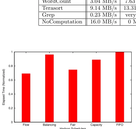
Figure 6: Elapsed time comparison. The FIFO
scheduler is the baseline. Nine jobs with 1GB in-put are submitted every 5 second.
Manger, and another one is for the name node of HDFS. For computing facilities, two clusters are in different network segment, and Cluster 1 has six nodes and Cluster 2 has five nodes. Regarding storage facilities, two data nodes of HDFS are in Cluster 1 and one is in Cluster 2. Each has around 30GB disk space and we set the replication number of HDFS to two.
5.2
Heterogeneous Cluster Setting
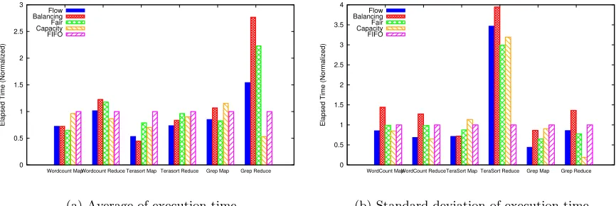
We analyze the behavior of our flow scheduler and other existing Hadoop schedulers. We compare Flow Scheduler with FIFO Scheduler, Fair Scheduler, and Capacity Sched-uler. Moreover, we create a Balancing Scheduler that dis-tributes the flow demand to computing facilities evenly. In this experiment, we setup a Hadoop system with Cluster 1 and Cluster 2. Then we submit jobs (Wordcount, Terasort and Grep) to the Hadoop system every five seconds. The wordcount and terasort job has an input size 1GB and we submit four times for each of them. Since the grep job has longer running time, we submit only one job with input size 1GB. As shown in Figure 6, FIFO Scheduler has the longest elapsed time and Flow Scheduler can complete all the jobs in a shorter time. Figure 7 shows that Flow Scheduler has lower average execution time of tasks in most of cases. Be-sides, Flow Scheduler demonstrates more smooth execution time of tasks, as shown in Figure 7(b), because Flow Sched-uler has lower values of the standard deviation of execution time.
5.3
Scheduling Overhead
At each scheduling run, we filter out the computing facil-ities without available slots, and then calculate the penalty cost of each arc in the min-cost flow network. This encoding is exported as an input to the solver to derive the optimal as-signment. The solver accounts most of scheduling overhead. The graph size in our experiment is greater than 100 at peak time (|T|>100 and|C|= 11). The maximum execu-tion time is around 97msand the minimum one is 2ms, and the average solving time is 8.3ms. For a large-scale graph size, as indicated in [19], the solving time of the min-cost flow optimization problem can be acceptable.
5.4
Discussion
In the traditional Hadoop model, data locality plays an important role in system performance so that most existing schedulers focus on maximizing the number of local map tasks. However, the decoupled Hadoop model does not have this property so that most existing schedulers does not fit in this model. From our experiments, we observed that those schedulers might assign tasks directly to the first node with available slots, which happens on FIFO Scheduler more of-ten. FIFO Scheduler first considers node-level data locality and then rack-level data locality. This scheduling method can cause problems because many tasks of a job would be assigned to a computing facility. This would lead to resource competition especially when high flow demand of tasks are executed on the same node. Figure 5 shows a similar result when multiple higher flow demand tasks are running on a node. The drop percentage appears to be the largest one for the NoComputation line.
The proposed flow scheduling tries to avoid the task as-signment that can affect the flow rate of processing. Our cost model considers the quality of data supply (Rsout and
Rcout) and the qualify of processing flow rate on
comput-ing facilities. We argue that maintaincomput-ing the flow rate of processing can increase the system throughput, and Figure 5 greatly support our argument. More interestingly, our flow scheduling method can somehow eliminate stragglers [13, 34]. Our result shows that Flow Scheduler derives more smooth execution time of map tasks.
0 0.5 1 1.5 2 2.5 3
Wordcount MapWordcount Reduce Terasort Map Terasort Reduce Grep Map Grep Reduce
Elapsed Time (Normalized)
Flow Balancing Fair Capacity FIFO
(a) Average of execution time
0 0.5 1 1.5 2 2.5 3 3.5 4
WordCount MapWordCount ReduceTeraSort Map TeraSort Reduce Grep Map Grep Reduce
Elapsed Time (Normalized)
Flow Balancing Fair Capacity FIFO
(b) Standard deviation of execution time
Figure 7: The average execution time and the standard deviation of execution time. Flow Scheduler shows more smooth execution time and this somehow suggests flow scheduling can eliminate stragglers that are caused by resource contention.
flow throughSW. We also construct another arc for com-puting facilities that connects toSW. In such a scenario, we cannot decide the cost for the arc fromSW toCmbecause
we lose the information of flow demand. For this reason, Quincy has a cost, zero, for the arc from the rack to com-puting nodes. In our cost model, we simply raise the cost of an arc that causes cross-rack communication. To address this problem, we probably can look into convex network op-timization that can support this scenario so as to delivering a more accurate cost model.
6.
RELATED WORK
6.1
The decoupled model
In previous work [30], the author compared the perfor-mance of Hadoop integrated with different types of storage architecture. The author found that in the split architecture, Hadoop has imbalance issue access to remote data storage, which can lead to poor I/O performance. In the following, we discussed the use cases that integrate Hadoop with sep-arate storage. After that, we describe scheduling methods for Hadoop and cluster that are related to our work.
6.1.1
Parallel File System
Several research studies show their interests in replacing HDFS with other high performance storage systems. W. Tantisiriroj et al [31] argues that parallel file systems can support diverse workloads and provides a better tradeoff be-tween performance and reliability. The authors proposed a PVFS shim layer to incorporate data layout of PVFS to achieve data locality. Maltzahn et al considered Ceph as a scalable alternative to HDFS [24], and they create a mapping layer which is similar to the PVFS one. GPFS is a shared-disked file system developed by IBM, and widely adopted in supercomputers. R. Ananthanarayanan et al [7] from IBM Research modify data layout in GPFS and expose this infor-mation to Hadoop. These are the earliest studies that tried to replace HDFS, but none of them considers optimizing Hadoop at the job scheduler level.
6.1.2
Enterprise Storage
Another research study [27] analyzed the feasibility to use a very powerful storage node to accommodate Hadoop, and he finds that Hadoop performance is dominated by the band-width between computing and storage facilities.
Recently, the researchers in NetApp Inc. argued that it is required to decouple compute and storage nodes in big data analytics because enterprise IT often deployssilosto manage high-value data [23]. The decoupled Hadoop model would incur high cost on data loading from the backend storage system to compute nodes. They propose MixApart, which includes the data-aware task scheduler, the task-aware data scheduler and a caching mechanism, to optimize Hadoop performance. However, they mainly focused on highly data-reuse workload.
6.1.3
Cloud Storage Service
Cloud computing has emerged as an important technol-ogy for the pay-as-you-go model [8, 20]. In such a plat-form, object storage, e.g. Amazon S3 and Azure Blob Stor-age, is primarily chosen for persistent data. Amazon Elastic MapReduce and Azure HDInsight are two popular Hadoop platforms on the cloud [1, 6]. Both cases enable Hadoop to support data access to object storage.
6.2
Resource and Job Scheduling
Hadoop has the builtin FIFO scheduler, which allocates resources based on first-come-first-serve policy and data lo-cality. The Fair Scheduler was originally developed by Face-book with the objective of resource sharing, and Yahoo pro-posed Capacity Scheduler to support fairness and priority sharing; both of them aim at achieving data locality and fairness in a large cluster. LATE [34] improvs the spec-ulative execution by accurately estimating the remaining time of tasks, which can better support Hadoop in heteroge-neous environment. HFS [33] uses delay scheduling to solve the conflict between data locality and fairness, and the job throughput can be improved by almost 2x. All of these schedulers are suitable for the Hadoop reference model but not the decoupled model.
profil-ing so that resource utilization can be increased. This work does not consider the decoupled Hadoop model, and the new Hadoop YARN supports flexible slot allocation; how-ever, their job profiling can be applied to our system. More-over, instead of choosing the optimal slot number, our flow scheduling can utilize resource more efficiently because com-puting facilities can maintain high processing flow rate.
A scheduling problem can be solved as the network op-timization problem. Quincy [19] adopts the min-cost flow network to achieve fair scheduling in a distributed commut-ing system. Our flow schedulcommut-ing is similar to this approach; however, our cost model is based on flow rate but not the data size that is required by a computing task. We believe flow rate is a better choice because it can be a good indicator to determine the type of a task. For example, a low flow rate task is a CPU-intensive task; however, the data size itself is not enough to determine the right task type. CAM [22] ar-gues that the decoupled model is not suitable for virtualized clouds, and it attempts to co-allocate data with virtual ma-chines. CAM utilizes the network topology information and builds the min-cost flow network to reconcile data placement and VM placement.
7.
CONCLUSION
The decoupled Hadoop model is flexible and much more preferable in many scenarios. However, existing Hadoop schedulers do not consider this model and hence the schedul-ing method fails to optimize the system throughput. Our flow scheduling method uses the penalty cost for task as-signments in order to increase the processing flow rate on computing facilities. We encode this problem as the min-cost flow problem and then we can obtain the optimal as-signment. We have implemented a pluggable Flow Sched-uler for Hadoop YARN and it supports the latest version of Hadoop. Our experiment results have shown that our flow scheduling can greatly improve the system throughput by about 30% so as to eliminate stragglers. These results support that the proposed flow scheduling can maintain the flow rate of processing.
Flow scheduling seems efficient for the decoupled model, but there still remains large space to improve. For our cur-rent implementation, Flow Scheduler requires job profile and machine profile, which is not practical. We believe we can estimate the flow demand of tasks and the flow capability of facilities at runtime. A naive approach is to sample the flow demand of a task and then use this information to decide the cost of the remaining tasks of the same job. Another approach is to monitor the flow rate of tasks so that we can adjust the penalty cost dynamically. We can also decide the flow capability of facilities in a similar way. Overall, we are positive about flow scheduling but more extensive evalua-tions have to be conducted before we can conclude.
8.
REFERENCES
[1] Amazon Web Services. http://aws.amazon.com/. [2] Capacity Scheduler.
http://hadoop.apache.org/docs/current/hadoop-yarn/hadoop-yarn-site/CapacityScheduler.html. [3] Fair Scheduler.
http://hadoop.apache.org/docs/current/hadoop-yarn/hadoop-yarn-site/FairScheduler.html. [4] The Hadoop project. http://hadoop.apache.org/.
[5] Virtual Computing Lab. http://vcl.ncsu.edu. [6] Windows Azure. http://www.windowsazure.com/. [7] R. Ananthanarayanan and K. Gupta. Cloud analytics:
Do we really need to reinvent the storage stack. In Proceedings of the 2009 conference on Hot topics in cloud computing, pages 1–5, 2009.
[8] M. Armbrust, A. Fox, R. Griffith, A. D. Joseph, R. Katz, A. Konwinski, G. Lee, D. Patterson,
A. Rabkin, I. Stoica, and M. Zaharia. A view of cloud computing.Communications of the ACM, 53(4):50–58, 2010.
[9] S. Babu. Towards automatic optimization of
MapReduce programs. InProceedings of the 1st ACM symposium on Cloud computing - SoCC ’10, page 137, New York, New York, USA, June 2010. ACM Press. [10] G. Bell, J. Gray, and A. Szalay. Petascale
computational systems.Computer, 39(1):110–112, Jan. 2006.
[11] J. Bresnahan, D. Labissoniere, T. Freeman, and K. Keahey. Cumulus : An Open Source Storage Cloud for Science. InProceedings of the 2nd international workshop on Scientific cloud computing, pages 25–31, 2011.
[12] M. Chowdhury, M. Zaharia, J. Ma, M. I. Jordan, and I. Stoica. Managing data transfers in computer clusters with orchestra. InProceedings of the ACM SIGCOMM 2011 conference, volume 41, pages 98–109, Oct. 2011. [13] J. Dean and S. Ghemawat. MapReduce : Simplified
Data Processing on Large Clusters. Inthe 6th Symposium on Operating Systems Design and Implementation (OSDI), pages 137–150, Dec. 2004. [14] I. Foster. Designing and Building Parallel Programs:
Concepts and Tools for Parallel Software Engineering. Jan. 1995.
[15] A. V. Goldberg. An Efficient Implementation of a Scaling Minimum-Cost Flow Algorithm.Journal of Algorithms, 22(1):1–29, Jan. 1997.
[16] Google. Google Cloud Platform. http://cloud.google.com/, 2012.
[17] W. Gropp, E. Lusk, and A. Skjellum.Using MPI: portable parallel programming with the
message-passing interface. MPI, 1999.
[18] M. Isard, M. Budiu, Y. Yu, A. Birrell, and D. Fetterly. Dryad: distributed data-parallel programs from sequential building blocks. InEuroSys, volume 41, pages 59–72, Mar. 2007.
[19] M. Isard, V. Prabhakaran, J. Currey, U. Wieder, K. Talwar, and A. Goldberg. Quincy: Fair Scheduling for Distributed Computing Clusters. InProceedings of the ACM SIGOPS 22nd symposium on Operating systems principles - SOSP ’09, page 261, New York, New York, USA, Oct. 2009. ACM Press.
[20] K. Kambatla, A. Pathak, and H. Pucha. Towards Optimizing Hadoop Provisioning in the Cloud. [21] R. T. Kouzes, G. A. Anderson, S. T. Elbert,
I. Gorton, and D. K. Gracio. The Changing Paradigm of Data-Intensive Computing.Computer, 42(1):26–34, Jan. 2009.
Applications in the Cloud. InProceedings of the 21st international symposium on High-Performance Parallel and Distributed Computing - HPDC ’12, page 211, New York, New York, USA, June 2012. ACM Press.
[23] Madalin Mihailescu, Gokul Soundararajan, and Cristiana Amza. MixApart: Decoupled Analytics for Shared Storage Systems. InHotCloud, 2012.
[24] C. Maltzahn, E. Molina-Estolano, A. Khurana, A. J., Nelson, S. A. Brandt, and S. Weil. Ceph as a scalable alternative to the Hadoop Distributed File System. http://static.usenix.org/publications/login/2010-08/openpdfs/maltzahn.pdf,
2010.
[25] C. Moler. Matrix Computation on Distributed Memory Multiprocessors. InHypercube Multiprocessors. 1986.
[26] J. Polo, C. Castillo, D. Carrera, Y. Becerra, I. Whalley, M. Steinder, J. Torres, and E. Ayguad´e. Resource-aware adaptive scheduling for MapReduce clusters. pages 180–199, Dec. 2011.
[27] G. Porter. Decoupling storage and computation in Hadoop with SuperDataNodes.ACM SIGOPS Operating Systems Review, 44(2):41, Apr. 2010. [28] L. Ramakrishnan, K. R. Jackson, S. Canon, S. Cholia,
and J. Shalf. Defining future platform requirements for e-Science clouds. InProceedings of the 1st ACM symposium on Cloud computing - SoCC ’10, page 101, New York, New York, USA, June 2010. ACM Press. [29] S. Sakr, A. Liu, D. M. Batista, and M. Alomari. A
Survey of Large Scale Data Management Approaches in Cloud Environments.IEEE Communications Surveys & Tutorials, 13(3):311–336, 2011.
[30] J. Shafer.A Storage Architecture for Data-Intensive Computing. PhD thesis, Rice University, 2010. [31] W. Tantisiriroj, S. Patil, G. Gibson, S. W. Son, S. J.
Lang, and R. B. Ross. On the duality of data-intensive file system design: Reconciling HDFS and PVFS. In International Conference for High Performance Computing, Networking, Storage and Analysis (SC)), pages 1–12, 2011.
[32] J. Wolf, D. Rajan, K. Hildrum, R. Khandekar, V. Kumar, S. Parekh, K.-L. Wu, and A. Balmin. FLEX: a slot allocation scheduling optimizer for MapReduce workloads. pages 1–20, Nov. 2010. [33] M. Zaharia, D. Borthakur, J. Sen Sarma,
K. Elmeleegy, S. Shenker, and I. Stoica. Delay scheduling: a simple technique for achieving locality and fairness in cluster scheduling. InProceedings of the 5th European conference on Computer systems -EuroSys ’10, page 265, New York, New York, USA, Apr. 2010. ACM Press.
[34] M. Zaharia, A. Konwinski, and A. Joseph. Improving mapreduce performance in heterogeneous
environments. InProceedings of the 8th USENIX conference on Operating systems design and implementation, pages 29–42, San Diego, California, 2008.