ABSTRACT
BAVGI, SAI KIRAN. Flow Diagnostics using Filtered Rayleigh Scattering. (Under the direction of Dr. Venkat Narayanaswamy).
Flow Diagnostics using Filtered Rayleigh Scattering
by Sai Kiran Bavgi
A thesis submitted to the Graduate Faculty of North Carolina State University
in partial fulfillment of the requirements for the degree of
Master of Science
Mechanical Engineering
Raleigh, North Carolina 2017
APPROVED BY:
_______________________________ Dr. Venkat Narayanaswamy
Committee Chair
DEDICATION
BIOGRAPHY
Sai Kiran Bavgi was born in Zaheerabad (in the state of Telangana), India in 1991. He pursued a Bachelor’s degree in Mechanical Engineering at Indian Institute of Technology Guwahati. After graduating in 2013, he joined FMC Technologies as a Design Analyst. Here he was involved in the design and analysis of various subsea oil and gas extraction products.
ACKNOWLEDGMENTS
First and foremost, I would like to thank my parents, sister and little brother for their love and support throughout my life.
I would like to sincerely thank my graduate advisor, Dr. Venkat Narayanaswamy for his constant guidance over the past two years. I similarly extend my gratitude to Dr. Chih-Hao Chang and Dr. Jack Edwards for serving on my thesis committee.
TABLE OF CONTENTS
LIST OF TABLES ... vii
LIST OF FIGURES ... viii
1 INTRODUCTION... 1
1.1 Background ... 2
1.2 Filtered Rayleigh Scattering (FRS) ... 5
1.3 Conceptual Approach ... 7
2 DESIGN OF EXPERIMENTS ... 12
2.1 Experimental setup for measuring transmission characteristics of molecular filter. 12 2.2 Experimental setup for FRS imaging Studies ... 17
2.3 Nd:YAG Laser Calibration ... 21
2.4 Pressure Vessel Design ... 25
2.4.1 Finite Element Analysis of Pressure Vessel ... 27
3 RESULTS AND DISCUSSION ... 29
3.1 Iodine Filter transmission studies ... 29
3.2 Theoretical estimation of pressure and molecular weight scaling... 32
3.3 Experimental Results... 46
3.3.1 Nitrogen temperature results ... 47
3.3.2 CO2 temperature results... 49
3.3.3 CH4 temperature results ... 51
3.3.4 Comparison of theoretical and experimental FRS signals ... 54
LIST OF TABLES
Table 1: Dynamic Viscosity and Thermal Conductivity values of N2... 35
Table 2: FRS Signal ratios of N2 for various combinations of pressure and temperature ... 39
Table 3: Dynamic Viscosity and Thermal Conductivity values of CO2 ... 42
Table 4: Dynamic Viscosity and Thermal Conductivity values of CH4 ... 42
Table 5: Dynamic Viscosity and Thermal Conductivity values of C2H4... 43
Table 6: Parameters for N2 temperature experiments ... 47
Table 7: Parameters for CO2 temperature experiments ... 50
Table 8: Parameters for CH4 temperature experiments ... 52
Table 9: Theoretical and molecular weight scaling for each frequency combination ... 60
LIST OF FIGURES
Figure 1: Filtered Rayleigh Scattering Concept using an Nd:YAG Laser and a molecular iodine
filter ... 5
Figure 2: RBS profiles at different y value ... 11
Figure 3: Schematic of experimental setup for measuring I2 cell transmission spectra ... 13
Figure 4: A photograph of the experimental setup for measuring transmission characteristics of I2 filter ... 15
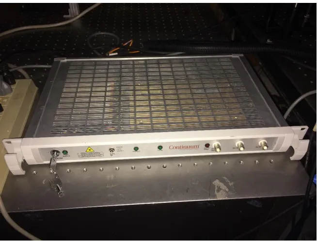
Figure 5: Continuum Surelite pulsed Nd:YAG laser ... 15
Figure 6: Continuum Injection seeder... 16
Figure 7: Iodine Cell and Temperature controller ... 16
Figure 8: Schematic of experimental setup for 2D FRS imaging studies and simultaneous monitoring of I2 cell transmission ... 17
Figure 9: (a) Heater setup, (b) Burner setup ... 19
Figure 10: A photograph of the layout of optical components for FRS imaging studies ... 20
Figure 11: Schematic of experimental setup for laser calibration ... 21
Figure 12: Vacuum cell [17] used for laser calibration ... 22
Figure 13: Observed normalized signal vs frequency plot ... 23
Figure 14: Iodine cell transmission calculated using Forkey code ... 24
Figure 15: Pressure vessel used for FRS imaging studies on gases at high pressures ... 26
Figure 16: NPT Sight Windows ... 26
Figure 28: Selected frequency locations for FRS imaging studies ... 46
Figure 29: Variation of FRS signal of N2 with temperature at different frequencies ... 48
Figure 30: Variation of FRS signal of N2 with frequency at different temperatures ... 49
Figure 31: Variation of FRS signal of CO2 with temperature at different frequencies ... 50
Figure 32: Variation of FRS signal of CO2 with frequency at different temperatures ... 51
Figure 33: Variation of FRS signal of CH4 with temperature at different frequencies ... 52
Figure 34: Variation of FRS signal of CH4 with frequency at different temperatures ... 53
Figure 35: Variation of normalized theoretical and experimental signals of N2 with temperature at different frequencies... 54
Figure 36: Variation of normalized theoretical and experimental signals of CO2 with temperature at different frequencies ... 55
Figure 37: Variation of normalized theoretical and experimental signals of CH4 with temperature at different frequencies ... 56
Figure 38: Experimental and theoretical FRS signal ratios at different frequency combinations ... 57
Figure 39: Experimental and theoretical FRS signal ratios at different frequency combinations ... 58
Figure 40: Experimental and theoretical FRS signal ratios at different frequency combinations ... 59
1 INTRODUCTION
In today’s world, substantial efforts are being made to improve the efficiency and cleanliness of energy conversion devices vital to modern life. In order to achieve this, there is significant ongoing research aimed towards improving our understanding of complex combustion phenomena. In combusting flows, having an accurate information of gas temperature holds the key to uncovering pollutant information, flame extinction and heat release.
Automotive engineers have designed internal combustion engines that no one believed were possible a mere 20 or 30 years ago. Today’s engines squeeze twice as much power out of their fuel and produce significantly less pollution. But having a better temperature measurement capability with high spatial, and temporal resolution can help them in further development of the combustion devices.
Conventional intrusive measurement devices such as thermocouples, thermistors, pressure probes, etc., disturb the flow under study and can be damaged by high temperature or pressure in the combustion environment. Although, it is clear that probe methods are cheap, inherently simple and easy to use, several questions are raised due to their lack of sufficient temporal and spatial resolution.
parameters. The advancements in these Laser-based diagnostic techniques over the past few decades have been reviewed in detail by Miles, Lempert and Forkey [1].
1.1 Background
Among current non-intrusive laser diagnostic techniques, there are few suitable for temporally resolved, two-dimensional temperature imaging in reacting flows. Rayleigh Scattering and planar laser-induced fluorescence (PLIF) are perhaps the most widely used techniques for temperature imaging in reacting flows.
Zelenak et al [15,17]. But they are not without drawbacks, (1) need to seed a fluorescing molecule or atomic species into the flame, (2) in turbulent sprays, the collected signal originates from both the gas and liquid phase of droplet. Therefore, the accuracy of any measurement will be predicated on the ability to accurately discriminate between the liquid-phase and vapor-liquid-phase fluorescence signal which cannot be spectrally separated. There are currently on-going efforts to rectify the phase-discrimination problem by combining PLIF with other techniques. However, the uncertainties in this approach are still quite high and, to date, there are no proven methodologies for completely isolating the vapor-phase information. Although the advancements in laser devices, camera sensors and computers over the past decade have led to increased resolution and accuracy of the measurements made by Laser based diagnostic techniques, there are number of situations where these traditional techniques are difficult to implement such as turbulent spray environments, investigating gas-phase mixing within spray flows, or any experimental setup where unwanted laser scattering is unavoidable. Development of laser-based diagnostic techniques that can obtain qualitative and quantitative information within these challenging environments is of particular interest to the scientific community.
Rayleigh-Brillouin scattering, while blocking unwanted scattering of laser light from background and particles.
1.2 Filtered Rayleigh Scattering (FRS)
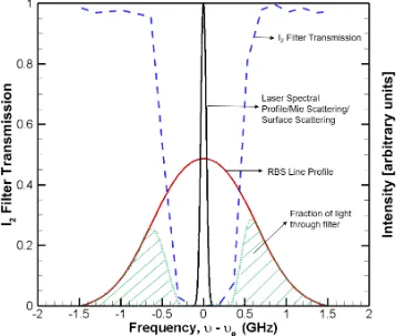
A schematic of the working principle behind FRS technique is shown in Figure 1. In a typical Rayleigh scattering experiment, the scattered light is comprised mainly of Rayleigh and Raman scattering from gas-phase molecules, Mie/Tyndall scattering from solid particles or liquid droplets, and scattering from the surface (e.g., windows, wall). The spectrum of each scattering process is broadened or shifted with respect to the laser based on the motion and properties of the scatterer.
Mie/Tyndall scattering from droplets or particles exhibit the same frequency distribution as the laser with a small spectral shift which is a function of their velocity. Scattered light from surface has the same frequency distribution as the laser. Raman scattering is due to inelastic scattering of photons by molecules which are excited to higher vibrational or rotational energy levels by incident laser. The scattered photons have higher or lower energy than incident photons which is manifested as a change in frequency of the scattered photon away from the incident laser. However, in the context of this work Raman scattering can be neglected since the signal is 102-103 times weaker than the Rayleigh scattering signal.
1.3 Conceptual Approach
The FRS signal collected at each pixel of the camera is a function of the flow velocity (𝑊), laser frequency (𝜈𝑜), pressure (𝑃), temperature (𝑇), gas composition, observation angle (𝜃), number density of the gas (𝑛), and laser intensity (𝐼𝑜). The transmitted FRS signal can be written as [10],
𝑺𝑭𝑹𝑺(𝑷, 𝑻, 𝑾, 𝝂, 𝜽) = 𝑪𝑰𝒐𝒏∅𝒊(𝑷, 𝑻, 𝑾, 𝝂, 𝜽) (1)
Where,
𝐶 is the constant associated with collection optics and imaging systems and ∅𝑖 is a FRS specific variable expressed as,
∅𝒊(𝑷, 𝑻, 𝑾, 𝝂, 𝜽) = (𝒅𝝈 𝒅𝜴⁄ )𝒊∫ 𝕽𝒊( 𝑷, 𝑻, 𝑾, 𝜽)𝝉(𝝂)𝒅𝝊 (2)
Where,
(𝑑𝜎 𝑑𝛺⁄ )𝑖− Differential Rayleigh Scattering cross section of species 𝑖,
ℜ𝑖 − Rayleigh-Brillouin Scattering lineshape for species 𝑖
𝜏 − Frequency dependent transmission of I2 cell
In order to account for the constant 𝐶, it is common to normalize the FRS signals by signal obtained at known reference condition. For example, at constant pressure, 𝑃, observation angle, 𝜃 and zero flow velocity; Normalized Eq. (1) can be written as:
𝑆𝐹𝑅𝑆(𝑇, 𝜈) 𝑆𝐹𝑅𝑆(𝑇𝑅𝑒𝑓, 𝜈)=
𝑇𝑅𝑒𝑓 𝑇 ×
∅𝑖(𝑇,𝜈)
Similarly, at constant Temperature, 𝑇, observation angle, 𝜃 and zero flow velocity; Normalized Eq. (1) can be written as:
𝑆𝐹𝑅𝑆(𝑃, 𝜈) 𝑆𝐹𝑅𝑆(𝑃𝑅𝑒𝑓, 𝜈) = 𝑃 𝑃𝑅𝑒𝑓× ∅𝑖(𝑃, 𝜈) ∅𝑖(𝑃𝑅𝑒𝑓, 𝜈)
In Eq. (3) and Eq. (4), the normalized FRS signal is represented by the product of two terms. The first term is the ratio of reference temperature and local temperature in Eq. (3), and in Eq. (4) the first term is the ratio of local pressure and reference pressure. The second term in both the equations is the ratio of convolution of Rayleigh-Brillouin lineshape (at local conditions) of species 𝑖 and frequency dependent I2 cell transmission to convolution of Rayleigh-Brillouin lineshape (at reference conditions) of species 𝑖 and frequency dependent I2 cell transmission.
If the density of gas is low or if the temperature is high enough, the spectral distribution of the scattered light is dominated by thermal motion of the molecules, because the mean free path of the molecules is large compared to the incident laser wavelength, and, so, the scattering just reflects the motion of the molecules themselves and takes the form of a Gaussian distribution given by [1],
𝑔(𝜃, 𝑇, 𝜈) = 2 Δ𝜈𝑇√
𝑙𝑛2
𝜋 𝑒𝑥𝑝 [−4𝑙𝑛2 ( 𝜈 Δ𝜈𝑇)
2 ]
Where, T is the absolute temperature, 𝜈 is the frequency, and Δ𝜈𝑇 is the FWHM of the profile (4)
Where, 𝑘𝐵 is Boltzmann constant, 𝑚 is molecular mass, and 𝑘 is defined as the scattering wave vector whose magnitude is given by
|𝑘| = 4𝜋 𝜆𝑠 𝑠𝑖𝑛 (
𝜃 2)
In Eq. (7), 𝜆𝑠 is the wavelength of incident laser and 𝜃 is the observation angle.
In gas kinetics, these low gas density or high temperature conditions correspond to Kundsen regime. On the other hand, when the mean free path length of the molecules reduces due to increase in gas pressure or drop in temperature, the scattering profile becomes increasingly controlled by the density fluctuations in the medium. These density fluctuations are caused due to acoustic waves travelling in the medium, which give rise to acoustic side bands in the scattering profile, also known as ‘Brillouin–Mandel’shtam scattering’. These conditions where mean free path length of the molecules is less than the laser wavelength correspond to hydrodynamic regime.
The RBS lineshape in this intermediate regime that consists of both random molecular motion and correlated motion due to travelling acoustic waves, can be computed using several models developed by number of researchers [11]; though the most widely used is the S6 model developed by Tenti et al. [12] and will be used in the context of this work.
These models all make use of a quantity called y-parameter which is defined as the ratio of laser source wavelength to mean free path of molecules and is given by
𝑦 ≡ 𝜆𝑠 2𝜋𝑙𝑚 ≅
𝑛𝑘𝐵𝑇 √2|𝑘|𝜗𝑜𝜂
(8)
Where, n is number density of the gas, 𝜆𝑠 is wavelength of the laser beam, 𝜂 is the shear viscosity, 𝑘𝐵 is Boltzmann constant, |𝑘| is the magnitude of scattering wave vector and 𝜗𝑜 is thermal velocity of molecules given by
𝜗𝑜 = √ 𝑘𝐵𝑇
𝑚
Figure 2 shows the Rayleigh-Brillouin scattering profiles of N2 calculated using Tenti S6 model for various y-parameters. It can be clearly seen that as the y-value increases the scattering profile transitions from symmetric Guassian distribution to a triple peaked profile with each peak having a Lorentzian shape, indicating a transition from Kundsen regime to hydrodynamic regime. On a side note, for N2 at standard atmoospheric conditions (1 atm, 298K) observed at 532 nm light, the y-parameter is around 0.8, indicating that the scattering is in intermediate regime and the acoustic effects cannot be neglected.
Figure 2: RBS profiles at different y value
2 DESIGN OF EXPERIMENTS
Two experimental configurations have been developed for the purpose of this study. The first configuration is for measuring the transmission profile of the molecular or atomic filter and later the observed transmission profile is compared with the transmission profile obtained from Forkey code calculations. The second configuration is used for FRS imaging studies and simultaneous monitoring of molecular or atomic filter’s transmission to ensure laser stability.
2.1 Experimental setup for measuring transmission characteristics of molecular filter
Figure 3: Schematic of experimental setup for measuring I2 cell transmission spectra
The 532 nm output is reflected off of a 45o mirror then passed through an iris onto a quartz glass flat. 85% of the laser beam transmitted through the glass flat goes to beam dump and the remaining 15% reflected beam passes through a half waveplate (orients the polarization of the beam) and a thin-film polarizer (transmits only P-polarized light). The combination of waveplate and the thin-film polarizer is used for further attenuation of laser beam energy. The beam then passes through an Iris and reflected off of a series of glass flats aligned at 45o to the beam path, the idea is to reduce the energy of the beam so that the photodiodes are not damaged. The reflected beam from the glass flat labeled as item 11 in Figure 3 is focused onto a diffuser and photodiode (Thorlabs, DET210, 1 ns rise time) assembly through a converging lens. The beam transmitted through the previous glass flat is again reflected off by a final glass flat and focused through a converging lens, temperature stabilized I2 cell, and onto a second diffuser and photodiode assembly. To ensure that the photodiodes do not pick up any scattered light/reflections from the surroundings, both the photodiodes and I2 cell were covered with laser-safe black hardboards which are not shown in the schematic.
2.2 Experimental setup for FRS imaging Studies
A schematic of the setup is shown in Figure 8. This experimental setup was developed for performing 2D FRS imaging studies on different gases at high pressures, high temperatures and premixed/diffusion flames. It also facilitates the simultaneous monitoring of I2 cell transmission to ensure laser stability.
Figure 8: Schematic of experimental setup for 2D FRS imaging studies and simultaneous monitoring of I2
The setup is hooked up with the same laser used for I2 cell transmission studies, frequency doubled (532 nm), injection-seeded, pulsed Nd:YAG laser, operating at 10 Hz repetition rate. The output from this laser is reflected off of a 45o-532 nm mirror onto a quartz glass flat (3). 15% of the beam reflected by the glass flat goes to the “monitor leg”. The monitor leg is used to ensure the stability of laser.
The reflected beam from the quartz glass flat is reflected off of a 45o-532 nm mirror then passes through an iris onto a quartz glass flat (6), 15% of the beam reflected by this glass flat passes through a half wave plate (orients the beam polarization) and a thin-film polarizer, the combination of which can be used to attenuate the pulse energy. The beam is then reflected off of a series of glass flats (9-12) aligned at 45o to the beam path to further attenuate the pulse energy. Finally, the beam is focused through a converging lens, temperature stabilized I2 cell, and onto a diffuser and photodiode assembly. The output signal from the photodiode is monitored on the digital oscilloscope. This arrangement helped in several aspects –the laser stability can be ensured before starting the experiments, any drift in the laser frequency can be observed while running the experiments over long periods and, can be used as a reference for FRS imaging studies.
The scattered light from the pressure vessel, (surface scattering from the walls, Raleigh scattering from the gas molecules) passes through a temperature stabilized I2 cell (1 torr partial pressure) and is finally collected by a CCD camera (PCO Pixelfly). Both the I2 cells are operated under starve-cell conditions at 313 K.
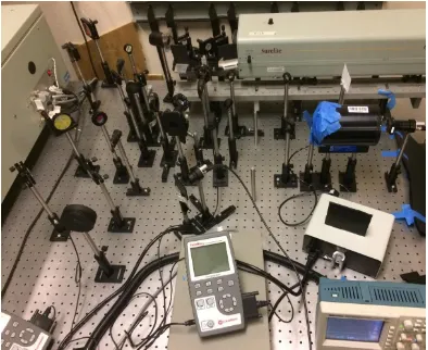
For conducting FRS imaging on gases at high temperatures or premixed/diffusion flames, the pressure vessel in the above setup can be replaced by a heater (Osram Air Heater) which can deliver high temperature gaseous flows, or the burner setup designed by Zelenak et al. [15] respectively. It is to be noted that while conducting FRS imaging on flames simultaneous Rayleigh scattering images were taken using a secondary CCD camera to normalize the FRS data of the flame with Rayleigh scattering data to account for energy fluctuations in the laser beam. The photographs of the experimental setup and the key components are shown in Figure 9-10.
2.3 Nd:YAG Laser Calibration
The Injection seeded Nd:YAG laser is tunable over a frequency range of 18793.018 – 18795.296 cm-1 according to the seed laser manual [16]. But in practice, it was observed to have some offset and had to be calibrated. The schematic of the setup used for calibrating the laser is shown in Figure 11.
Figure 11: Schematic of experimental setup for laser calibration
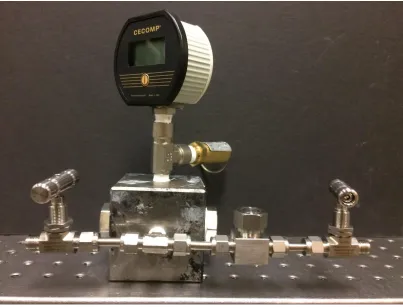
stainless steel flanges which hold the windows in place and are used for attaching vacuum pump, gas lines, thermocouple and a pressure transducer as shown in Figure 12.
Figure 12: Vacuum cell [17] used for laser calibration
Scattered light from the cavity walls passes through a temperature stabilized I2 cell and collected by a Princeton Instruments PI-MAX 4 ICCD camera, whose acquisition is aligned with the laser trigger.
normalized by FRS image with highest signal. Figure 13 shows the observed normalized signal vs frequency plot.
Figure 13: Observed normalized signal vs frequency plot
Figure 14: Iodine cell transmission calculated using Forkey code
Even though the frequency output of the laser was thermally tunable over a specified range of 18793.018 – 18795.296 cm-1, in practice, only the region highlighted Figure 14 (18793.50 – 18793.77 cm-1) was found to be stable for long periods of time.
2.4 Pressure Vessel Design
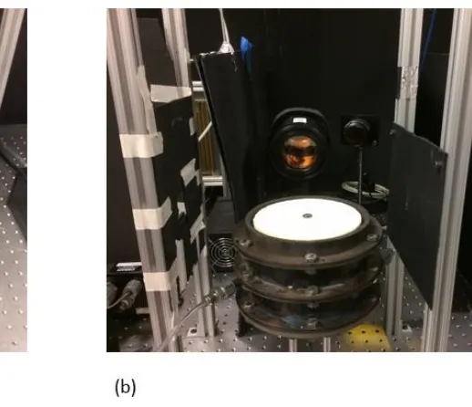
The pressure vessel shown in Figure 15, is specially designed to perform FRS imaging studies on gasses at high pressures. It comprises of:
1. A 4140-multipurpose alloy steel housing that has a high yield strength of 85000 psi and dimensions 3’’x3’’x3’’,
2. Three NPT (3/4’’) sight glasses. The sight glass consists of Corning fused silica 7980 optical window encased in a stainless-steel housing as shown in Figure 16. These sight glasses can withstand an internal pressure of 3040 psi (206.85 atm) and an external pressure of 145 psi (9.86 atm),
Figure 15: Pressure vessel used for FRS imaging studies on gases at high pressures
2.4.1 Finite Element Analysis of Pressure Vessel
A linear finite element analysis was performed in Ansys 17.1 to validate that the pressure vessel can with stand a pressure of 1500 psi. The simplified half-symmetry FE model used and the loading, boundary conditions are shown in Figure 17.
2.4.1.1 FEA Results
Figure 18: von Mises stress plot at 1500 psi
Figure 18 shows the von Mises stress distribution in the pressure vessel at 1500 psi internal pressure. The maximum von-Mises stress observed is around 6600 psi which is way below the yield strength of the material (85000 psi). This indicates that the pressure vessel is designed with a factor of safety of around 12.8 if the operating pressure is 1500 psi (~102 atm). However, the pressure vessel will be used to hold gases at maximum pressure of only 50 atm.
3 RESULTS AND DISCUSSION
In this study, the first step was to measure the transmission profiles of the molecular filters and compare them against the theoretical model. Subsequent analysis focusing on the development of pressure and molecular weight scaling of FRS signal ratios for different species theoretically and comparing it with the experimental results.
3.1 Iodine Filter transmission studies
Having an accurate information about the transmission spectra of the molecular filters being used is very critical in the context of FRS imaging studies. In this work two Iodine filters have been used, which have same path length of 125 mm and are operated at 313 K, but each has a different vapor pressure, 0.5 torr and 1 torr. These measurements were made possible using the experimental setup shown in Figure 3.
The transmission spectra were measured over a frequency range of 18793.11-18793.35 cm-1 (which covers two peak Iodine transitions) by tuning the Nd:YAG laser’s frequency. It should be noted that the photo diodes were calibrated by controlling the beam energy using the half-waveplate and thin film polarizer setup before doing the transmission experiments.
Two sets of experiments were conducted separately to measure the transmission profiles of the two iodine cells. Figure 19 and Figure 20 show the measured transmission profile for 1 torr and 0.5 torr iodine cells respectively. Also shown is the theoretical transmiss ion profile obtained using Forkey code. The abscissa is presented in terms of Optical Depth, which is simply a logarithmic representation of transmission given by, 𝑂𝐷 = −𝑙𝑜𝑔10(𝑡𝑟𝑎𝑛𝑠𝑚𝑖𝑠𝑠𝑖𝑜𝑛).
Figure 19: Measured transmission profile of the I2 cell with 125 mm path length, operated at 313 K and
Figure 20: Measured transmission profile of the I2 cell with 125 mm path length, operated at 313 K and
0.5 torr vapor pressure, using an injection seeded, pulsed, frequency doubled Nd:YAG laser. Also shown is the theoretical absorption profile at the same cell conditions
as the ratio of the energy contained within single longitudinal mode to that of the total pulse energy. Several studies have been carried out in the past, in an attempt to gain more knowledge about injection seeded lasers [18, 19]. More recent studies by Patton and others [20, 21], demonstrated that using an external air-spaced etalon improved the OD by more than two orders of magnitude. In this work, similar attempts have been made using an external solid-etalon, however, no significant improvements have been observed in the OD and hence, it has been avoided.
3.2 Theoretical estimation of pressure and molecular weight scaling
This section elucidates the strategy used to theoretically find pressure and molecular weight scaling of FRS signal ratios for various species. Four different, most commonly observed gases (N2, CO2, CH4, C2H4) in a typical combustion study were investigated in this work.
Figure 21: RBS profile of N2 shown at two extreme locations of selected frequency scan region at 1 atm
gas pressure and 600 K temperature. Also shown is the theoretical I2 transmission for a cell of path
length 125 mm, 1 torr vapor pressure and operated at 313 K
Subsequently, the FRS signal at each frequency step has been computed for all the temperature and pressure combinations by taking the convolution of RBS lineshape and I2 transmission spectrum.
instance, an increase of gas pressure from 1 to 50 bar will only resul t in 10% change of the shear viscosity [22]. The temperature dependent dynamic viscosity and thermal conductivity can be calculated using the Sutherland formulae [23] given by
𝜂 𝜂𝑜 = ( 𝑇 𝑇𝑜) 3/2𝑇 𝑜 + 𝑆𝜂 𝑇 + 𝑆𝜂 And 𝜅 𝜅𝑜 = ( 𝑇 𝑇𝑜) 3/2𝑇 𝑜 + 𝑆𝜅 𝑇 + 𝑆𝜅
Where, 𝑆𝜂 and 𝑆𝜅 are effective temperatures, called the Sutherland constants, which are gas specific, 𝑇𝑜 is the reference temperature, 𝜂𝑜 is the dynamic viscosity of the gas at reference temperature, and 𝜅𝑜 is the thermal conductivity of the gas at reference temperature
The dynamic viscosity and thermal conductivity values computed for N2 using the Sutherland formulae over a temperature range of 300 K – 2000 K are shown in Table 1.
(10)
Table 1: Dynamic Viscosity and Thermal Conductivity values of N2
Temperature, K Dynamic Viscosity, kg/m.s Thermal Conductivity, W/m.K
300 1.79E-05 0.026193
400 2.21E-05 0.032994
500 2.58E-05 0.039017
600 2.91E-05 0.04445
900 3.75E-05 0.058329
1200 4.45E-05 0.069847
1500 5.06E-05 0.079866
1800 5.61E-05 0.088835
2000 5.94E-05 0.094366
The value of the second coefficient of viscosity or “bulk-viscosity” is not very well known but in a study by Ziyu Gu [24], it was observed that the bulk viscosity scales similar to the dynamic viscosity with temperature. In this work, values at 300 K are taken from the literature and scaled at higher temperature. Also, in another study by Thomas A. McManus [25], an assessment of the sensitivity of the calculated RBS profiles to the bulk viscosity was conducted and it showed minimal sensitivity to the RBS profiles for the majority of species and temperature conditions.
The Tenti S6 model is considered to be most accurate for diatomic gases and low number density, but as pointed out by Young and Kattawar [26], even that model is not exact. However, in this work, the S6 model is used for all species (N2, CO2, CH4, and C2H4) even at high number density and an attempt has been made to validate it through experimental results.
on pressure, temperature and molecular weight. It is important to find how to scale these ratios with respect to above three parameters, which is a challenging task.
Figure 22: RBS profiles of N2 at two selected frequency locations, (a) 18793.35 cm-1 and (b) 18793.21 cm-1
at 1 atm and 600 K. Also shown is the theoretical I2 transmission spectrum for a cell of path length
125 mm, 1 torr vapor pressure and operated at 313 K
Figure 23: Convoluted scattering profiles of N2 at two selected frequencies at 1 atm gas pressure and
600 K.
Table 2: FRS Signal ratios of N2 for various combinations of pressure and temperature
Nitrogen Pressure (atm)
0.2 1 6 12 20
Temperature (K)
600 2.01727 2.01654 2.06916 2.1884 2.48791 900 1.86422 1.86256 1.85557 1.85333 1.87684
1200 1.74368 1.73693 1.71947 1.69836 1.67253
1500 1.63491 1.63549 1.61629 1.59196 1.56607
1800 1.5758 1.5722 1.55551 1.53329 1.51766
2000 1.52367 1.52004 1.50047 1.47378 1.45542
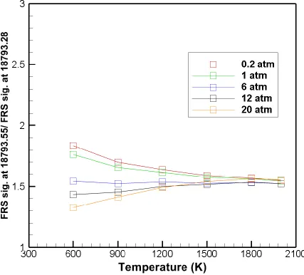
Figure 25: Variation of the FRS signal ratio of nitrogen with temperature and pressure for a bad choice of frequency pair (18793.55 cm-1 and 18793.28 cm-1)
Table 3: Dynamic Viscosity and Thermal Conductivity values of CO2
Temperature, K Dynamic Viscosity, kg/m.s Thermal Conductivity, W/m.K
300 1.50E-05 0.01659
400 1.93E-05 0.024381
500 2.33E-05 0.032592
600 2.69E-05 0.041058
900 3.62E-05 0.067047
1200 4.39E-05 0.092904
1500 5.07E-05 0.118033
1800 5.68E-05 0.142229
2000 6.05E-05 0.157813
The dynamic viscosity and thermal conductivity values of carbon dioxide are calculated using Sutherland formulae, eq. 10 and eq. 11 respectively.
Table 4: Dynamic Viscosity and Thermal Conductivity values of CH4
Temperature, K Dynamic Viscosity, kg/m.s Thermal Conductivity, W/m.K
300 1.31E-05 0.0344
400 1.67E-05 0.05
500 2E-05 0.0684
600 2.3E-05 0.0886
900 3.08E-05 0.1536
1200 3.72E-05 0.2185
1500 4.28E-05 0.2792
1800 4.78E-05 0.34
2000 5.09E-05 0.375
Table 5: Dynamic Viscosity and Thermal Conductivity values of C2H4
Temperature, K Dynamic Viscosity, kg/m.s Thermal Conductivity, W/m.K
300 1.05E-05 0.0206
400 1.36E-05 0.0366
500 1.64E-05 0.0526
600 1.89E-05 0.0686
900 2.55E-05 0.1166
1200 3.1E-05 0.1646
1500 3.57E-05 0.2126
1800 4E-05 0.2606
2000 4.27E-05 0.3086
The dynamic viscosity values of methane gas are calculated using the Sutherland formula, eq. 10, whereas the thermal conductivity values are taken from [21].
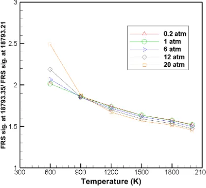
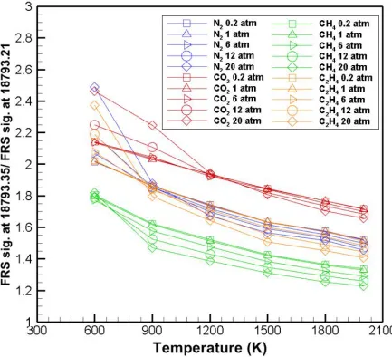
Figure 26 Variation of the FRS signal ratios of various species with temperature and pressure for the selected frequency pair (18793.35 cm-1 and 18793.21 cm-1)
exponents for pressure and higher exponents for molecular weight were tested and the best scaling was found to be:
𝑃−0.01×𝑀0.4
Where, P (atm) is the gas pressure and M (g/mol) is the molecular weight of the gas. Figure 27 shows the best collapsed P-T curves after applying the above power law.
3.3 Experimental Results
3.3.1 Nitrogen temperature results
At each of the five frequency locations, the FRS images of nitrogen were acquired over a temperature range of 300-800 K using the heater setup. The laser was given enough time to stabilize at each frequency location before acquiring the scattering images and the stability was continuously monitored using the monitor leg of the experimental setup discussed in section 2.2. All the experimental parameters are tabulated in Table 6.
Table 6: Parameters for N2 temperature experiments
Q-Switch delay 240 𝜇𝑠
Pulse Energy 140 mJ
Pulse frequency 10 Hz
N2 Flow rate 75 SLPM
Gas temperature range 300 – 800 K
Frequency Locations (cm-1) 18793.11, 18793.18, 18793.21, 18793.28, and 18793.35
Figure 29: Variation of FRS signal of N2 with temperature at different frequencies
higher temperatures and some portion of the broadened RBS profile enters the I2 absorption band and gets absorbed, which leads to lower difference in FRS signal at away from absorption and FRS signal at absorption locations.
Figure 30: Variation of FRS signal of N2 with frequency at different temperatures
3.3.2 CO2 temperature results
Table 7: Parameters for CO2 temperature experiments
Q-Switch delay 240 𝜇𝑠
Pulse Energy 140 mJ
Pulse frequency 10 Hz
CO2 Flow rate 75 SLPM
Gas temperature range 300 – 800 K
Frequency Locations (cm-1) 18793.11, 18793.18, 18793.21, 18793.28, and 18793.35
Figure 32: Variation of FRS signal of CO2 with frequency at different temperatures
3.3.3 CH4 temperature results
Table 8: Parameters for CH4 temperature experiments
Q-Switch delay 240 𝜇𝑠
Pulse Energy 140 mJ
Pulse frequency 10 Hz
CO2 Flow rate 75 SLPM
Gas temperature range 300 – 800 K
3.3.4 Comparison of theoretical and experimental FRS signals
Figure 36: Variation of normalized theoretical and experimental signals of CO2 with temperature at
different frequencies
Figure 37: Variation of normalized theoretical and experimental signals of CH4 with temperature at
3.3.5 Estimation of molecular weight scaling from experimental results
To estimate the molecular weight scaling from experimental results, firstly, FRS signal ratios at all possible frequency combinations of the five selected frequencies have been evaluated for three gases (N2, CO2 and CH4) as illustrated in Figure 38 to Figure 40, also shown is the theoretical FRS signal ratio for comparison.
Figure 40: Experimental and theoretical FRS signal ratios at different frequency combinations
Table 9: Theoretical and molecular weight scaling for each frequency combination
Frequency Combination Molecular weight scaling
for experimental data
Molecular weight scaling for theoretical data
18793.35/18793.28 𝑀0.34 𝑀0.45
18793.35/18793.21 𝑀−0.38 𝑀0.14
18793.35/18793.18 𝑀0.39 𝑀0.53
18793.35/18793.11 𝑀0.64 𝑀0
18793.21/18793.28 𝑀0.8 𝑀0.3
18793.21/18793.18 𝑀0.77 𝑀0.39
18793.18/18793.28 𝑀−0.04 𝑀0
18793.11/18793.28 𝑀1.02 𝑀0.48
18793.11/18793.21 𝑀0.59 𝑀0.18
18793.11/18793.18 𝑀1.35 𝑀0.56
Figure 43: Experimental and theoretical scaled FRS signal ratios at different frequency combinations
Table 10: Power law fit each frequency combination, where 𝑹 is the scaled signal ratio
Frequency Combination Power Law
18793.35/18793.28 𝑅 = 𝐸𝑥𝑝(−0.3812×𝑙𝑛(𝑇) + 2.144)
18793.35/18793.21 𝑅 = 𝐸𝑥𝑝(0.2319×𝑙𝑛(𝑇) + 0.5284)
18793.35/18793.18 𝑅 = 𝐸𝑥𝑝(−0.2016×𝑙𝑛(𝑇) + 0.5858)
18793.35/18793.11 𝑅 = 𝐸𝑥𝑝(0.1543×𝑙𝑛(𝑇) + 1.523)
18793.21/18793.28 𝑅 = 𝐸𝑥𝑝(−0.6129×𝑙𝑛(𝑇) + 1.331)
18793.21/18793.18 𝑅 = 𝐸𝑥𝑝(−0.4338×𝑙𝑛(𝑇) + 0.05976)
18793.18/18793.28 𝑅 = 𝐸𝑥𝑝(−0.1795×𝑙𝑛(𝑇) + 1.523)
18793.11/18793.28 𝑅 = 𝐸𝑥𝑝(−0.5354×𝑙𝑛(𝑇) + 0.4758)
18793.11/18793.21 𝑅 = 𝐸𝑥𝑝(0.1771×𝑙𝑛(𝑇) − 2.836)
3.3.6 Validation of the estimated Power-Law fits
The power law fits estimated at all frequency combinations in the previous section have been tested by conducting FRS experiments on diffusion and premixed flames. Flame experiments were conducted with an in-house designed, reconfigurable jet flame in co-flow or premixed flat flame burner. Further details describing the burner design can be found in Zelenak et al. [15].
Figure 45: Computed radial temperature profile across the laminar diffusion flame at an axial location of 15 mm above the jet exit, also shown is the temperature profile found by Zelenak e t al. [15]
The jitter in the signal, as well as the asymmetric signal profile, and the difference seen in the temperature profile from present study and previous studies can be attributed to:
1. Poor background calibration,
4 CONCLUSION AND FUTURE WORK
In this study, a novel and simple laser diagnostic strategy based on Filtered Rayleigh Scattering was developed to estimate the temperature of gaseous flows. On the outset, previous studies on laser scattering techniques were presented and the short-comings of these theories were briefly discussed. This was followed by the introduction of FRS and the conceptual approach involved in FRS process. Different optical layouts and components were designed to facilitate:
1. The laser calibration
2. Optical depth measurement of I2 vapor filter
3. FRS imaging studies on gases at different pressures and, temperatures 4. FRS imaging studies on flames
A systematic approach was taken to implement and test the hypothesized FRS strategy, which is summarized below:
1. Based on the theoretical estimation of FRS signals, it was found that the ratio of signals at 18793.35 cm-1 and 18793.21 cm-1 showed least variation with pressure and molecular weight of gas.
2. The laser was calibrated using the calibration setup and the stable working region was found. All the FRS imaging studies were performed across this region.
estimated and a temperature dependent power law was fitted through the scaled data points at each frequency combination.
5. FRS experiments on diffusion and premixed flames were conducted to test the temperature dependent power laws. It was observed that the radial temperature profiles across both the flames calculated using the ratio of FRS signals at 18793.18 – 18793.28 cm-1 frequency combination showed the best agreement with previous studies.
It is acknowledged that the major sources of error in radial temperature profile across the flame were due to the error in background calibration and the fluctuation in laser beam between the pulses.
4.1 Future work
Some of the major points of focus in future research to make this technique much more reliable and certain or improve would be:
1. Improving the robustness of the technique: by conducting FRS experiments on wide range of gases and finding a better frequency combination and a robust molecular weight scaling. Also, conducting experiments over a higher temperature range would give a more reliable power law fit.
2. Finding a pressure scaling just like the molecular weight scaling by conducting FRS experiments over a range of gas pressures.
5 REFERENCES
[1] Miles, R. B., Lempert, W. R. & Forkey, J. N., 2001. Laser Rayleigh Scattering.
Measurement Science and Technology, Volume 12, pp. R33-R51.
[2] Abhyankar, K., 1996. Hundred and twenty-five years of Rayleigh. Q. J. R. Astron. Soc. 37, p. 281.
[3] Fourguette, D. C., Zurn, . R. M. & Long, M. B., 1986. Two-dimensional Rayleigh thermometry in a turbulent nonpremixed methane–hydrogen flame. Combustion Science and Technology, 44(5-6), pp. 307-317.
[4] Dibble , R. W., Long, . M. B. & Masri , A., 1985. Dynamics of flames and reactive systems.
Progress in Astronautics and Aeronautics.
[5] Seitzman, J. M., Kychakoff, . G. & Hanson, R. K., 1985. Instantaneous temperature field measurements using planar laser-induced fluorescence. Optics Letters, 10(9), p. 439.
[6] McMillin, B. K., Palmer, J. L. & Hanson, R., 1993. Temporally resolved, two-line fluorescence imaging of NO temperature in a transverse jet in a supersonic cross flow.. Applied optics, 32(36), pp. 7532-45.
[8] Forkey, J. N., n.d. "Development and demonstration of filtered Rayleigh scattering—a laser based flow diagnostic for planar measurements of velocity, temperature, and pressure". Ph.D. dissertation (Princeton University, Princeton, N.J., 1996)
[9] Forkey, J. N., Lempert, W. R. & Miles, R. B., 1997. Corrected and calibrated I2 absorption model at frequency-doubled Nd:YAG laser wavelengths. Appl. Opt., Volume 36(27), pp. 6729-6738.
[10] Forkey, J. N. et al., 1994. Volumetric imaging of supersonic boundary layers using filtered Rayleigh scattering background suppression. IAA 32nd Aerospace Sciences Meeting Exhibit. (Reno, NV) paper AIAA 94-0491
[11] Pan, X. P., Shneider, M. N. & Miles, R. B., 2004. Coherent Rayleigh-Brillouin scattering in molecular gases. Phys. Rev. A, Volume 69, pp. 1-16.
[12] Tenti, G., Boley, C. D. & Desai, R. C., 1974. On the Kinetic Model Description of Rayleigh-Brillouin Scattering from. Canadian Journal of Physics, Volume 52, pp. 285-290.
[13] Elliot, G. S., Glumac, N. & Carter, C. D., 2001. Molecular Filtered Rayleigh Scattering Applied to Combustion. Meas. Sci. Tech, Volume 12(4), pp. 452-466.
[17] Zelenak, D., Sealy, W. & Narayanaswamy, V., 2016. Collisional broadening of Kr transition with combustion species as collision partners. Journal of Quantitative Spectroscopy & Radiative Transfer 174, pp. 28-38.
[18] Park, Y., Giuliani, G. & Byer, R., 1984. Single axial mode operation of a Q-switched Nd:YAG oscillator by injection seeding. IEEE Journal of Quantum Electronics, Volume 20(2), pp. 117-124.
[19] Barnes, N. P. & Barnes, J. C., 1993. Injection Seeding I: Theory. IEEE Journal Of Quantum Electronics, Volume 29(10), pp. 2670-2683.
[20] Patton, R. A., n.d. "Characterization and Improvements of Filtered Rayleigh Scattering Diagnostics". Masters Thesis (Ohio State University, 2013).
[21] Patton, R. A. & Sutton, J. A., 2013. Developement of Gas-Phase Mixing Measurements in Turbulent Spray Flows Using Filtered Rayleigh Scattering. Grapevine, Texas.
[22] White, F. M., 1998. Fluid Mechanics. s.l.:Mcgraw-Hill Series in Mechanical Engineering.
[23] White, F. M., n.d. Viscous Fluid Flow. s.l.:McGraw-Hill, Inc
[24] Gu, Z., n.d. "Spontaneous Rayleigh-Brillouin Scattering on Atmospheric Gases". Ph.D. dissertation (Vrije Universiteit Amsterdam, 2015).
[25] McManus, T. A. & Sutton, J. A., 2017. Quantitative 2D Temperature Imaging in Turbulent Nonpremixed Jet Flames using Filtered Rayleigh Scattering.
[27] Huber, M. L. & Harvey, A. H., n.d. Thermal Conductivity of Gases, s.l.: National Institute of Standards and Technology.
[28] Uribe, F. J., Mason, E. A. & Kestin, J., 1990. Thermal Conductivity of Nine Polyatomic Gases at Low Density. Journal of Physical and Chemical Reference Data, Volume 19, pp. 1123-1136.