Influence of Azimuth and Radial Neutron and Thermal Sources Anisotropy on Contact Problem Simulation in Real Fuel Pellet-Cladding Configuration Using FEM

18th International Conference on Structural Mechanics in Reactor Technology (SMiRT 18) Beijing, China, August 7-12, 2005 SMiRT18-C03-5

INFLUENCE OF AZIMUTH AND RADIAL NEUTRON AND

THERMAL SOURCES ANISOTROPY ON CONTACT PROBLEM

SIMULATION IN REAL FUEL PELLET-CLADDING

CONFIGURATION USING FEM

Josef Běláč, Mojmír Valach, Jiří Zymák

Nuclear Research Institute Rez plc, Czech Republic

Abstract

1. Introduction

The necessary assumption of wide nuclear energy development is to keep and to increase the nuclear fuel safety. On the other hand there is an aim to operate NPP’s economically. Importance of nuclear fuel as a basic part of each NPP is more and more apparent, so the effort of our work is to describe more correctly the behaviour of the cylindrical fuel rods under more stringent operational conditions obviously achieving high burn up. It implies, that modern fuel rod computer models are required to predict a “margin” to cladding tube integrity loss under normal operation and operational transients more reliably. One of the critical moments, which occur during the fuel duty, is pellet – cladding contact (and also modified pellet – pellet contact after a thermo-mechanical interaction). The difficulty of the contact event modelling can be documented by very simple example: one core in one loading of one reactor contains ~ 104 fuel rods, each fuel rod contains ~ 102 fuel pellets …where, when and how and in what detail we have to predict and to model it.

2. Unilateral contact

Mathematical modelling of unilateral contact problems is quite new area in applied mathematics; practical realization of it indicates next application of the finite element method (FEM). The principle of the method is based on the fact that a zone of unilateral contact of two solid bodies need not be defined a priori; its correct definition is one of the results of the solved problem.

The classical analysis of this problem, started by Herz in 1896 was limited to simple geometries. The age of high-speed computers brought qualitative change also into the analysis of the contact problems. On the basis of suitable discretization – by means of finite differences or FEM – the problems can be solved approximately even for complex geometrical situations and boundary conditions. As a technical problem A. Signorini originally formulated it in 1933 for the case of unilateral contact of an elastic body with the ideal rigid and smooth basis (so called Signorini’s problem). From the mathematical point of view the unilateral contact problem performs the application of variational inequalities, which form today the basis of the convex analysis and form the connection between mathematical physics problems and optimization ones. Instead of classical variational equations the solution of variational inequalities is not found on the whole function space but on some closed part of it. The problem tends to seek the conditional extreme of the functional of deformation energy. These problems are non-linear ones due to not only existing material non-linearities but also by the set on which the solution is being found and which can alter during the solution process.

Let two bodies occupy the bounded regions Ω′,Ω ′′ with Lipschitz boundaries. In the following, one or two primes denote, that the quantity is referred to the body Ω′and Ω ′′, respectively. Let x=

(

x1,x2

)

be Cartesian coordinates. We seek the displacement vector field u=

(

u1,u2

)

over Ω′∪Ω ′′ , i.e. u′=

(

u1′,u′2

)

on Ω′ and u′′=

(

u1′′,u2′′

)

on Ω ′′ and the associated strain tensor field eij. The stress tensor τij is related to the strain tensor by means of the generalized Hooke’s law. The stress tensor satisfies the equation of equilibrium in

Ω ′′ ∪

Ω′ and some (classical) conditions on boundaries ∂Ω′∪∂Ω ′′ of the domains

Ω = Ω ′′ ∪

Ω‘

Ω‘‘ ΓK

Γτ

Γ0

Γu

Now we shall focus on the parts of the domains Ω′∪Ω ′′, where a possible contact may occur. We distinguish two classes of contact problems, as follows: 1. bounded contact zone, 2. enlarging contact zone, which differ significantly by the character of the contact. For the reason of simplicity let us consider now the case of zero friction.

2.1 Bounded contact zone

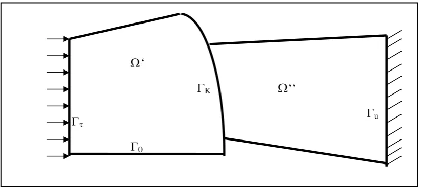
First let us consider the case, when the contact zone cannot enlarge during the deformation process. Such an assertion is determined by the geometrical shape of the two bodies in a neighbourhood of he possible contact zone (Fig. 1).

Fig. 1 Illustration of unilateral contact with bounded contact zone

Let the body Ω ′′ be fixed on a part Γ_uof its boundary, let the surface traction be prescribed on a part Γ_τ of the body Ω′, let the condition of the axis symmetry is defined on a part Γ0 of the body Ω′. Hence we may define the contact zone ΓK =∂Ω′∩∂Ω ′′. We say that a unilateral bounded contact occurs on ΓKif

0 u

u_n′ + _n″≤ (1)

holds on Γ_K , where u_n′ =u_i′⋅n_i′, u_n″=u_i″⋅n_i″ are projections of displacement

components into the outward unit normal ⎟

⎠ ⎞ ⎜

⎝

⎛ ′ ′

=

′ n₁ ,n₂

n , n′′=−n′ corresponding to the sets

Ω ′′

Ω′, (summation convention is used over the repeating index). The condition (1) means non-penetrating of both bodies.

Next let us consider the contact forces. By virtue of the law of action and reaction we have

″ = ′

t t T

T , T_n′=T_n″ on ΓK.

0 T Tt t =

″ = ′

, Tn Tn ≤0

″ = ′

.

Altogether, we define the boundary conditions on ΓKas follows:

0 u un n ≤

″ + ′

, Tn Tn ≤0

″ = ′

, (2)

0 T u

un n n =

′ ⋅ ⎟ ⎠ ⎞ ⎜ ⎝

⎛ ′ ₊ ″ _{, (3)}

0 T Tt t =

″ = ′

. (4)

The equation (3) means that at points without contact no contact force may occur.

2.2 Enlarging contact zone

In some important cases the contact zone can enlarge during the deformation process. Such a situation occurs if two bodies Ω′ and Ω ′′ have smooth boundaries in a neighbourhood of ΓK =∂Ω′∩∂Ω ′′ . Then we must change the definition of the contact condition. Let us consider the case of Fig. 2. We place a coordinate system (ξ, η) in such a way that the ξ-axis coincides with the direction of n′′and η -axis with the common tangent of ∂Ω′and ∂Ω ′′ at a “central” point P∈∂Ω′∩∂Ω ′′.

Fig. 2 Illustration of unilateral contact with enlarging contact zone

The Fig.2 corresponds with the situation before the deformation. The parts of ∂Ω′and ∂Ω ′′, which come into a contact during the deformation process, can be estimated as follows:

( )

( )

{

, ;a b, fM

}

, M '," M

K = ξ η ≤η≤ ξ= η =

Γ ,

Ω‘ Ω‘‘

a

b

ΓK‘‘

ΓK‘

ξ η

where f′,f′′ are continuous on a,b . (The interval has to be chosen a priori.) Arguing similarly as in the previous section, we are led to the following condition:

( )

a,b

u

u_ξ″− _ξ′≤εη ∀η∈ , (5)

where ε

( )

η =f′

( )

η −f′′

( )

η is the distance of the two boundaries before deformation; ″

′

ξ ξ ,u

u are projections of the displacement vectors into the direction of (positive) ξ-axis.

Using also the law of action and reaction, we come to the conditions

(

cos ′

)

1 = ″

(

cos ′′

)

1 ≤0 ′

− _α − _α −

ξ

ξ T

T , (6)

0 T

Tη′= η″ = , (7)

0 = ″ ⋅ ⎟ ⎠ ⎞ ⎜ ⎝ ⎛ ″ ₋ ′ ₋ ξ ξ

ξ u ε T

u , (8)

which hold at all points of ΓK′∪ΓK″ with the same coordinates η∈ a,b . Here

(

cos

)

1 , ',"

2 / 1 2 1 = ⎟ ⎟ ⎠ ⎞ ⎜ ⎜ ⎝ ⎛ ⎟⎟ ⎠ ⎞ ⎜⎜ ⎝ ⎛ + = − M d dfM M η α , αM

is being the angle between η-axis and the tangent to M K

Γ , respectively. The condition (8)

follows from this consideration: at points without contact, i. e. if u_ξ″−u_ξ′−ε<0 , no

contact force may occur, i. e. T_ξ′ =T_ξ″=0. The conditions (7) approximate the zero friction

– after neglecting the projection M M sin T_ξ ⋅ α .

2.3 Variational formulation

A variational formulation – principle of minimum potential energy – can be associated to the above-mentioned unilateral contact problems. Instead of the standard variational formulations, the unilateral contact problems minimize the functional

L(v) = 1/2 A(v, v) - L(v), (9)

on the set of admissible displacements K, which fulfills the relation (1) in the case of bounded contact zone and relation (5) in the case of enlarging contact zone. The quadratic part of the functional L

A(v, v) =

∫

( ) ( )

Ω

ε

τ . dx

is the strength energy of the bodies (Ω′∪Ω ′′=Ω), the linear part L(v) =

∫

Ω

dx v .

F_{i i} +

∫

τ

Γ

dS v .

P_{i i} is the work of the body forces and of the surface tractions.

A function u∈K is called a weak (variational) solution of the unilateral contact problem, if

L(u) ≤ L(v) ∀v ∈ K. (10)

Due to the fact that the set K does not form the whole space but only his closed subset, the variational inequality (10) does not tend to a system of linear equations. It has to be solved as a bonded extreme problem – to seek the minimum of the functional L on the set K.

Each numerical realisation of the particular unilateral contact problem leads to a system of linear equations, which has to be solved. This system is not directly connected with the derivation of the functional but results from applied numerical method for the solving of nonlinear optimization problems (method of Lagrangian multipliers, conditional conjugate gradients method, Newton-Raphson method, etc.).

2.4 Available tools used for the modelling

The problem has been solved by means of the COSMOS/M software system. It is a complete, modular finite element system, which includes for instance modules to solve linear and nonlinear static problems in addition to problems of heat transfer. Developing a reliable model capable of predicting the behaviour of structural systems represents one of the most difficult problems to face the analyst. The FEM provides an effective vehicle for performing these problems due to its versatility and the great advancement in its adaptation to computer use. The success of a finite element analysis depends largely on how accurately the geometry, the material behaviour and the boundary conditions of the actual problem are idealized. One has to take into consideration that all real structures are nonlinear in some way. In addition, the unilateral contact problems are nonlinear due to their optimization substance as was mentioned above. The unilateral contact forms the basis for adequate pellet-cladding modelling and it was used in all calculated problems.

3. Results of pellet-cladding modelling

Several results of 2D (r-ϕ) pellet-cladding modelling are introduced in this chapter. All presented cases were solved as the steady state problems with nonzero friction and with sliding. You can see the basic dimensions of considered fuel rod components in Tab. 1.

Tab. 1 Basic dimensions of considered fuel rod components.

fuel rod inner radius [m] 0,7 ⋅10-3

fuel rod outer radius [m] 3,84⋅10-3

cladding inner radius [m] 3.86⋅10-3

cladding outer radius [m] 4,55⋅10-3

fuel pellet height [m] 10⋅10-3

The initial pellet-cladding P-C radial gap was set 20 μm for the data from Tab. 1 to simulate a P-C contact.

3.1 Creating of cladding oxide model

The ZrO2 material with its temperature dependent material properties was created in COSMOS/M library by use of the MATPRO-SCDAP material library. The ZrO2 scale is used to simulate partially burned nuclear fuel. The first calculations with the both sided cladding oxide layers were performed. Each oxide thickness of 25 μm was used; the rest thickness of the metal clad was set of 50 μm smaller. The radial temperature profiles of fuel rod with bilateral clad oxidation in both models (r-z) and (r-ϕ) are shown in Fig. 3 and Fig. 4.

Fig. 3 Radial temperature profile of (r-z) fuel rod model with bilateral oxidation and with P-C contact

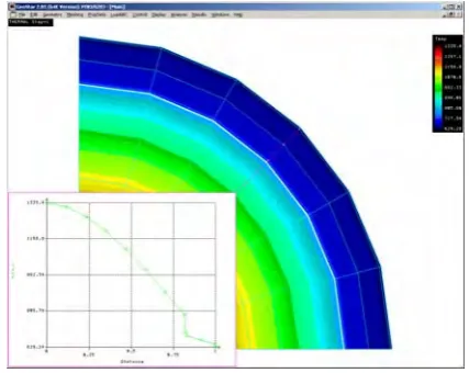
Fig. 4 Radial temperature profile of (r-ϕ) fuel rod model with bilateral oxidation and

Maximum calculated temperatures are 1334.9 K and 1335.4 K, respectively.

Let us introduce the example with non-uniform cladding oxidation. Now, let us assume that the oxide layer occurred on the clad inner side at the point where the local P-C contact was appeared at first. The oxide layer at clad outer side is assumed uniform. Meshing of the (r-ϕ) segment is in Fig. 5. The oxide layers are dark; the clad metal layer is light. Due to the symmetry, the example solves the problem with two opposite inner oxide layers (Fig. 6).

Fig. 5 Example of non-uniform cladding oxidation

Fig. 6 The complete example of non-uniform inner clad oxidation

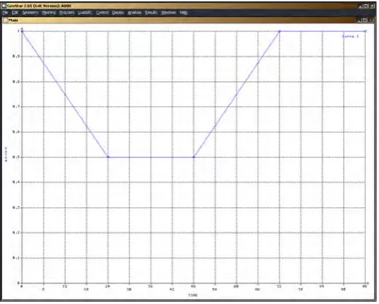
Let us consider the time dependent linear heat rate with its maximum value 300 W/cm, the time profile of it [hour] is in Fig. 7, the linear heat rate is in relative units.

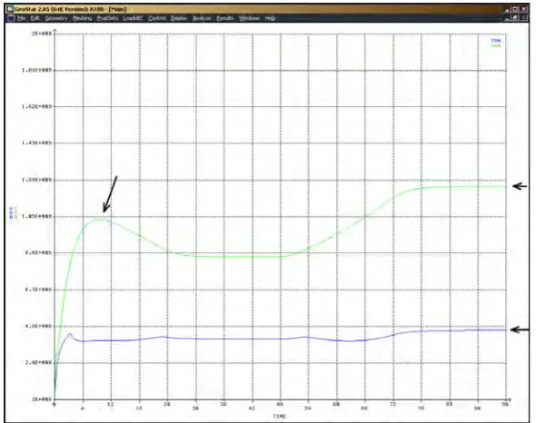
Right low detail of Fig. 5 is in Fig. 8. There are two nodes (No. 56 and No. 79), where the effective stresses are illustrated.

Fig. 8 Nodes No. 56 and No. 79, where the effective stress is demonstrated

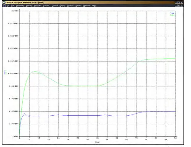
Result of non-linear thermo-mechanical calculation with, so called, “nominal data” – the time profile of the effective stress in two significant nodes (see Fig. 8) is shown in Fig. 9.

3.2 Various types of inhomogeneities or anisotropy

We will compare the results mentioned above with the similar ones but created with some in-homogeneities in input data and in boundary conditions. Let us assume three types of in-homogeneities, see Fig. 10:

Fig. 10 Illustration of assumed types of in-homogeneities

a) 80% of heat rate value in radial fuel pellet segment standing “against” the inner oxide layer;

b) 80% of cladding creep deformation increment value in analogous radial segment of metal, c) 80% of the convection coefficient value in the analogous part of the cladding outer

boundary.

Results of the three cases in the same nodes as before are shown in Figs. 11, 12, 13.

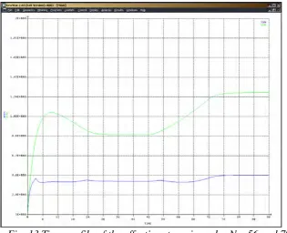
Fig. 12 Time profile of the effective stress in nodes No. 56 and 79 computed with 80% of cladding creep deformation increment value (case b)

Fig. 13 Time profile of the effective stress in nodes No. 56 and 79 computed with 80% of the convection coefficient value (case c)

changes. Detailed differences among the effective stresses at the end of calculations for the four computed cases are in Tab. 2.

Tab. 2 Effective stress value at the end of each calculation, node No. 79, element No. 67 (Fig. 8)

type of calculation effective stress [MPa]

nominal 479

case a 459

case b 474

case c 483

4. Conclusion

The method and calculation results of 2D (r-ϕ) contact elasto-thermal-creep solutions of pellet-cladding configuration with non-symmetric sources and various boundary conditions were presented. All calculations have been performed by means of the COSMOS/M software system. The formerly developed non-linear, thermal dependent material properties were applied. The an-elastic fuel and cladding material behaviours were treated; the clad creep model was used. These steps will be related to the cladding crack (crack growth and crack stability) modeling, too. All considered contact problems were solved with prescribed friction coefficient between the pellet-cladding contact regions, including of the structures sliding.

5. Acknowledgement

6. References

[1] TIMOŠENKO, Š.: Strength of Materials I., II. Technicko-vědecké vydavatelství, Praha 1951. (in Czech)

[2] HLAVÁČEK, I., HASLINGER, J., NEČAS, J., LOVÍŠEK, J.: Solution of Variational Inequalities in Mechanics. Alfa, Bratislava 1982. (in Slovak)

[3] HINTON, E., OWEN, D. R. J.: Finite Element Programming. AP, London 1977.

[4] COSMOS/M 2.5 for Windows - online manuals, SRAC 1999.

[5] COSMOS/M 2.8 for Windows - online manuals, SRAC 2003.

[6] HAGRMAN, D. L. at al.:SCDAP/RELAP/MOD3.1 – MATPRO, NUREG/CR-6150, EGG-2720, Idaho,1993.

[7] VALACH, M., ZYMÁK, J., MIASNIKOV, A.: Open questions on the “interface” between classical fuel behaviour modelling and detailed 3D mechanistic simulation using Finite Element Method. TRANSURANUS Users Club Meeting, 22-23 September 2003, paper of NRI Rez plc, UJV 11943-T, M.

List of figures:

Fig. 1 Illustration of unilateral contact with bounded contact zone ... 490

Fig. 2 Illustration of unilateral contact with enlarging contact zone... 491

Fig. 3 Radial temperature profile of (r-z) fuel rod model with bilateral oxidation and with P-C contact ... 494

Fig. 4 Radial temperature profile of (r-ϕ) fuel rod model with bilateral oxidation and with P-C contact ... 494

Fig. 5 Example of non-uniform ... 495

Fig. 6 The complete example of ... 495

Fig. 7 Time profile [hour] of linear heat rate [1]... 495

Fig. 8 Nodes No. 56 and No. 79, where the effective stress is demonstrated ... 496

Fig. 9 Time profile of the effective stress in nodes No. 56 and 79 ... 496

Fig. 10 Illustration of assumed types of in-homogeneities... 497

Fig. 11 Time profile of the effective stress in nodes No. 56 and 79 ... 497

Fig. 12 Time profile of the effective stress in nodes No. 56 and 79 ... 498