Leading-Edge Flow Sensing for Aerodynamic Parameter Estimation.

ABSTRACT

VISWANATH SIDDHANTHI. Leading-Edge Flow Sensing for Aerodynamic Parameter Estimation (Under the direction of Dr. Ashok Gopalarathnam.)

Real-time estimation of air-data parameters such as airspeed, angle of attack and lift coefficient at various sections of an aircraft wing or turbine blade is highly beneficial for continuous performance monitoring. The continuous tracking of aerodynamic parameters in aircraft could not only facilitate early detection of any problems but will also help maintain a greater sense of control, prevent dangerous stall situations and enhance operating capabilities. Current methods of flow sensing include electromechanical self-orienting vanes, air-data booms or flush air data sensing (FADS). Although effective, the methods are incapable of measuring sectional air-data parameters.

In order to achieve this, a novel Leading-Edge Flow Sensing (LEFS) algorithm was developed in recent research for unflapped airfoils. This thesis aims to test the applicability of the algorithm to airfoil cases with flaps extended. For the algorithm to be applicable for usage in aircraft, it must be capable of computing the required data at different sections of the wing in not only cruise with flaps retracted, but also during takeoff and landing where the flaps are extended. This thesis also explores the applicability of the algorithm to airfoils with slotted flaps which are commonly found on most commercial aircraft.

The thesis analyzes five airfoils: S809, NLF(1)-0414, NLF(1)-0215, NACA 0012 and NACA 23012 with a simple flap configuration set to different angles of deflection. The thesis also analyzes one multi-element airfoil, UIUC 1600, with a flap deflection of 36 degrees. The flap element of the multi-element airfoil was separately analyzed by placing the pressure ports on the leading-edge of the flap. The pressure data for each of the airfoils was obtained from wind-tunnel test results or CFD analysis. In each case, the algorithm was able to successfully predict the air-data parameters.

Leading-Edge Flow Sensing for Aerodynamic Parameter Estimation

by

Viswanath Siddhanthi

A dissertation submitted to the Graduate Faculty of North Carolina State University

in partial fulfillment of the requirements for the degree of

Master of Science

Mechanical Engineering

Raleigh, North Carolina 2019

APPROVED BY:

_________________________________ _________________________________ Dr. Matthew Bryant Dr. Kenneth Granlund

_________________________________ Dr. Ashok Gopalarathnam

ii

DEDICATION

iii

BIOGRAPHY

iv

ACKNOWLEDGEMENTS

First and foremost, I would like to thank my advisor Dr. Ashok Gopalaratnam for giving me an opportunity to work under him and for guiding me through the thesis. I am also thankful for the grader positions and an opportunity to design the turbine models for one of his project proposals. All the work done under him gave me a lot of work experience in different fields. I am also grateful to Dr. Matthew Bryant and Dr Kenneth Granlund for being on my thesis committee.

I would like to thank Dr. Aditya Saini whose research work formed the basis for my thesis and for the guidance and help with understanding the concepts and procedure to run the algorithms. Next, I would like to thank the members of my research group: Pranav, Shreyas, Vishnu, Ethan and Hari for the help along the way. I thank my roommates Arjun, Prakhar and Yash for helping me out with everything and making me feel at home. I would also like to thank my managers, Deloris Griffin and Ocean DeMarco for the all the help and support.

I would like to extend a special thank you to my fiancée Ms. Deepthi Ayalasomayajula for the constant help and motivation in the last six years. Thank you for bearing with me and constantly reviewing my work. All this wouldn’t have been possible without your love and support.

v

TABLE OF CONTENTS

LIST OF TABLES . . . vii

LIST OF FIGURES . . . viii

LIST OF SYMBOLS . . . xi

Chapter 1 Introduction . . . 1

1.1 Leading Edge Flow Sensing . . . 5

1.2 Thesis Outline . . . 6

Chapter 2 Background and Setup . . . 8

2.1 Theory and concepts . . . 8

2.1.1 Leading edge parabola . . . 9

2.1.2 Potential flow and Conformal mapping . . . 10

2.2 Methodology . . . 12

2.2.1 Parabola fitting . . . 13

2.2.2 Selection of pressure ports . . . 16

2.2.3 Non-linear regression . . . 17

2.2.4 Computing results .. . . 18

Chapter 3 Simple flap airfoil analysis . . . 20

3.1 NREL Wind tunnel: S809 . . . . . . . 20

3.2 Natural Laminar flow (NLF) Airfoils . . . 24

3.2.1 NLF(1) - 0414 . . . 25

3.2.2 NLF(1) - 0215 . . . 29

3.3 NACA Airfoil Series . . . 32

3.3.1 Meshing . . . 32

3.3.2 CFD . . . 34

3.3.3 NACA 0012 . . . . 36

3.3.4 NACA 23012 . . . 39

Chapter 4 Multi-element airfoil analysis . . . 43

4.1 Meshing . . . 45

4.2 CFD . . . 46

4.3 Results . . . . 49

Chapter 5 Conclusions . . . 53

5.1 Future work . . . 54

REFERENCES. . . 56

APPENDIX. . . 59

Appendix Airfoil Coordinates. . . 60

A.1 S809. . . 60

vi

A.3 NLF(1)-0215 . . . 65

A.4 NACA 0012 (Closed trailing edge) . . . 68

A.5 NACA 23012 (Closed trailing edge) . . . 71

A.6 UIUC 1600 . . . 74

A.6.1 Main element . . . 74

vii

LIST OF TABLES

Table 1 Pressure port locations on the S809 airfoil . . . 21

Table 2 Pressure port locations on the NLF(1) - 0414 airfoil . . . 25

Table 3 Pressure port locations on the NLF(1) - 0215 airfoil . . . 29

Table 4 Properties of air . . . . . . . . . . 32

Table 5 Pressure port locations on the NACA 0012 airfoil . . . . 36

Table 6 Pressure port locations on the NACA 23012 airfoil . . . 39

Table 7 Airfoil Parameters . . . . . . . 44

Table 8 CFD parameters . . . . . . . . 47

Table 9 Main element pressure ports . . . . . . . 49

Table 10 Pressure port locations for rotated flap coordinates with chord along x-axis . . . .50

viii

LIST OF FIGURES

Figure 1.1 Pitot Static sensor. Image source: https://www.nasa.gov/sites/default/files/

atoms/files/aero-intro-physics_0.pdf. . . 3

Figure 1.2 Angle of attack sensor. Image source: https://ntrs.nasa.gov/archive/nasa/ casi.ntrs.nasa.gov/20140011419.pdf . . . . 3

Figure 1.3 A conventional air-data boom for measuring pressures and flow angles. [1,2] . 3 Figure 1.4 Flush Air Data System installation at the nose of the F-18 Systems Research Aircraft [12,13] . . . 4

Figure 2.1 Combination of two flow sources . . . 9

Figure 2.2 Stagnation point flow [1,2] . . . 11

Figure 2.3 Stagnation point flow transformed to flow past a parabola [1,2] . . . 12

Figure 2.4 Parabola fit for NACA0012 . . . . 14

Figure 2.5 NACA0012 . . . 14

Figure 2.6 Parabola fit for S809 . . . 15

Figure 2.7 S809 . . . 15

Figure 2.8 Parabola fit for NLF(1) – 0414 . . . 16

Figure 2.9 NLF(1) – 0414 . . . 16

Figure 2.10 A comparison of the XFOIL pressure distribution with the pressure distribution over the leading edge parabola for (a) S809 at an angle of attack of 5 degrees and (b) NLF(1)-0414 at an angle of attack of 5 degrees . . . . 18

Figure 2.11 LEFS summary . . . 19

Figure 3.1 S809 flap/aileron configurations [22] . . . 21

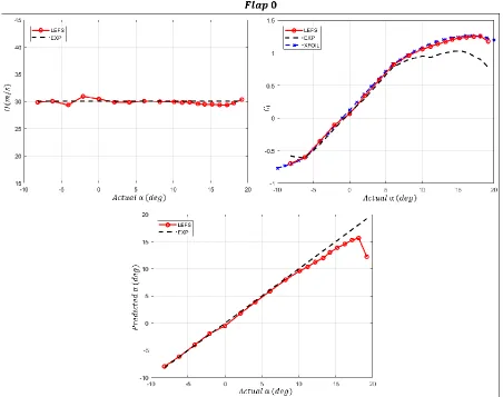
Figure 3.2 Comparison of velocity, angle of attack and lift coefficient from LEFS and wind tunnel, for Re = 1 million for S809 with no flap . . . 22

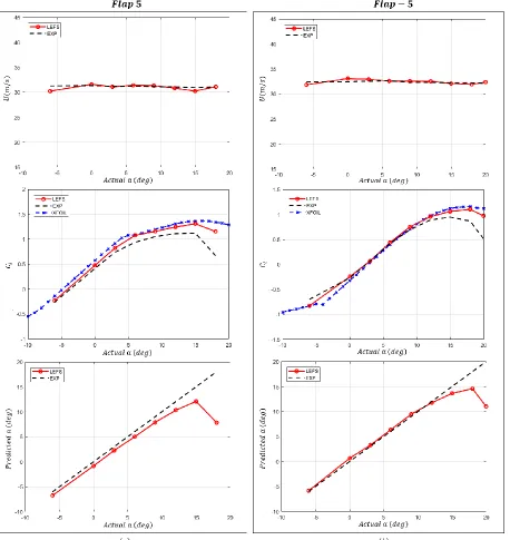
Figure 3.3 Comparison of velocity, lift coefficient and angle of attack from LEFS and wind tunnel, for Re = 1 million (a) S809 with 5 degrees of flap (b) S809 with -5 degrees of flap . . . . 23

Figure 3.4 Comparison of velocity, angle of attack and lift coefficient from LEFS and wind tunnel, for Re = 1 million with -10 degrees of flap . . . 24

Figure 3.5 NLF(1) – 0414 airfoil with laminar flow up to x/c = 0.7 . . . 25

Figure 3.6 Comparison of velocity, lift coefficient and angle of attack from LEFS and wind tunnel, for Re = 3 million (a) NLF(1)-0414 with no flap (b) NLF(1)- 0414 with 5 degrees of flap . . . 26

Figure 3.7 Comparison of velocity, lift coefficient and angle of attack from LEFS and wind tunnel data (a) NLF(1)-0414 with 10 degrees of flap at a Re = 3 million (b) NLF(1)-0414 with -5 degrees of flap at a Re = 6 million . . . 27

ix

Figure 3.10 Comparison of velocity, lift coefficient and angle of attack from LEFS and wind tunnel data at a Re = 6 million for (a) NLF(1)-0215 with no flap and

(b) NLF(1)-0215 with 10 degrees of flap . . . 30

Figure 3.11 Comparison of velocity, lift coefficient and angle of attack from LEFS and wind tunnel data at Re = 6 million for NLF(1)-0215 with -10 degrees of flap . 31 Figure 3.12 Inflation layers . . . 33

Figure 3.13 (a) NACA 0012 airfoil with 5 degrees of flap (b) NACA 23012 with 5 degrees of flap . . . 34

Figure 3.14 x vs CP plots from CFD results at alfa 0 (a) NACA 0012 airfoil with 5 degrees of flap (b) NACA 0012 airfoil with 10 degrees of flap (c) NACA 0012 airfoil with -5 degrees of flap (d) NACA 23012 with 5 degrees of flap (e) NACA 23012 with 10 degrees of flap (e) NACA 23012 with -5 degrees of flap . . . 35

Figure 3.15 NACA 0012 airfoil . . . . 36

Figure 3.16 Comparison of velocity, lift coefficient and angle of attack from LEFS and CFD results at a Re = 3 million for (a) NACA 0012 with no flap and (b) NACA 0012 with 5 degrees of flap . . . 37

Figure 3.17 Comparison of velocity, lift coefficient and angle of attack from LEFS and CFD results at a Re = 3 million for (a) NACA 0012 with 10 degrees of flap and (b) NACA 0012 with -5 degrees of flap . . . 38

Figure 3.18 NACA 23012 airfoil . . . 39

Figure 3.19 Comparison of velocity, lift coefficient and angle of attack from LEFS and CFD results at a Re = 3 million for (a) NACA 23012 with no flap and (b) NACA 23012 with 5 degrees of flap . . . 40

Figure 3.20 Comparison of velocity, lift coefficient and angle of attack from LEFS and CFD results at a Re = 3 million for (a) NACA 23012 with 10 degrees of flap and (b) NACA 23012 with -5 degrees of flap . . . 41

Figure 4.1 Slotted flaps. Image source: https://history.nasa.gov/SP-468/ch10-5.htm . . . 43

Figure 4.2 UIUC 1600 two element airfoil 47 Figure 4.3 flap angle . . . 44

Figure 4.4 Meshed UIUC 1600 . . . 46

Figure 4.5 Inflation layers on main and flap element . . . 46

Figure 4.6 x vs CP plots from CFD results at angle of attack of -5 . . . 48

Figure 4.7 x vs CP plots from CFD results at angle of attack of 0 . . . 48

Figure 4.8 x vs CP plots from CFD results at angle of attack of 5 . . . 49

Figure 4.9 Comparison of velocity, lift coefficient and angle of attack from LEFS and CFD data at Re = 3 million for the multielement airfoil UIUC 1600 . . . 50

x

Figure 5.1 Leading edge high lift devices. Image source: https://history.

nasa.gov/SP-468/ch10-5.htm . . . 55 Figure 5.2 Leading edge slats on the Boeing 737. Image source:

xi

LIST OF SYMBOLS

A Multiplicative factor of order one

a'

Parameter relating to the stagnation point location c Airfoil chord

C1 Main element chord (multi-element airfoil) C2 Flap element chord (multi-element airfoil) Cl Lift coefficient

Cd Drag coefficient Ci Camber coefficient Cf Skin friction coefficient

CFD Computational Fluid Dynamics FADS Flush Air Data Sensing

LEFS Leading Edge Flow Sensing LUT Lookup tables

NLF Natural Laminar Flow P Local static pressure Po Stagnation pressure

Pi Pressure at ith pressure port P∞ Freestream pressure r Nose radius

Re Reynolds number RMS Root mean square Ti Thickness coefficient T Temperature

xii α Angle of attack

δ Flap angle ρ Density

λ Initial slope of camberline 𝜑 Velocity potential

Ψ Stream function θ Ideal angle

μ Dynamic viscosity

1

Chapter 1

Introduction

Accurate measurement of air-data parameters is important in many areas such as flight testing, aircraft control, monitoring the performance of turbines etc. Real-time measurement of air-data parameters on flights can prevent dangerous stall situations and provide enhanced control of the aircraft. These parameters include the airspeed (U∞), angle of attack (α) and sectional lift coefficient (Cl) and drag coefficient (Cd).

Extensive wind tunnel testing and flight testing of the aircraft is performed before its development which is costly and time consuming. But there are certain aspects of the process that could be made more efficient [3]. An algorithm capable of estimating aerodynamic parameters in real time during such flight testing could not only be used for data collection but also as a tool for making a decision to continue or abort the test based on the data collected or from a safety perspective.

2

In the case of birds, there is an abundant sensory data transferred to the central nervous system from the wing using gradually adapting receptors associated with propagational covert feathers, alular joints and vibration receptors in the follicles of secondary feathers [6]. For example, the peregrine falcon uses vibration magnitude as sensory stimulus to the mechanoreceptors for sensing the angle of incidence when diving [7]. Thus, the falcon which adapts a streamlined V-shape when diving, uses this information to control its attitude to be in the narrow window of safe angle of incidence.

The ability to freely interact with the surroundings in order to gather crucial information in real time could pave way for a new generation of intelligent aircraft with enhanced control capabilities and attendant benefits to health monitoring and improved flight efficiency. Having an algorithm that continuously measures the local angle of attack and lift coefficient at different locations on a wing can prevent dangerous and uncontrollable stalls by aiding the pilots in early diagnosis of the situation. Flow sensing is also extremely useful in multiple other fields such as wind tunnel tests and monitoring the operating conditions of devices such as wind turbines where there is uncertainty in the sectional operating conditions because of unknowns associated with rotational effects, wind speeds and gradients, elastic twist and induced inflow. Conventional methods for flow sensing include electromechanical self-orienting vanes [8,9], air-data booms, or flush air data sensing (FADS). Although these methods are successful, they have certain drawbacks. Air-data booms come in multiple configurations: some capable of measuring pitot static pressure requiring separate sensors for angle of attack and side slip while others may be capable of measuring all the three parameters. Pitot-static sensors and angle-of-attack sensors are shown in Figures 1.1 and 1.2 respectively.

3

Figure 1.1: Pitot Static sensor. Image source:

https://www.nasa.gov/sites/default/files/atoms/files/aero-intro-physics_0.pdf

Figure 1.2: Angle of attack sensor. Image source:

https://ntrs.nasa.gov/archive/nasa/casi.ntrs.nasa.gov/20140011419.pdf

4

Flush Air Data Sensing (FADS) systems were developed in response to problems associated with air-data booms. In this technology, pressure readings are obtained through an array of ports on the nose cone of the aircraft which make them completely non-intrusive. But this approach has its drawbacks associated with the numerical instabilities experienced by the semiempirical models that are used to process the FADS pressure signals. Additionally, since the pressures are measured on the outer surface of the aircraft, locally induced flows complicate the calibration of the devices [2,12,13]. The flush air data sensing system for the F-18 Systems Research Aircraft shown in Figure 1.4.

Figure 1.4: Flush Air Data System installation at the nose of the F-18 Systems Research Aircraft [12,13].

FADS are usually mounted in proximity of the fuselage nose, but aerodynamic parameters can also be obtained using pressure sensors mounted on airfoil skin [11,10]. However, the sensing technology and data processing are complicated and unlike in the case of an aircraft nose cone, the complex design of avionics needed cannot easily be housed in the wing.

5

to develop the relationship between input from the sensor array and the output aerodynamic parameters: air speed, angle of attack and angle of sideslip [11,15].

Recently, vision-based tracking of aircraft states is being explored in micro air vehicles. This approach involves estimating the state of the aircraft on a real-time basis from a set of tracked feature points using an implementation of the extended Kalman filter [16,17,18]. Such methods however have high costs associated with them and the optical sensors are highly susceptible to damage.

Flow sensing is not only useful in the field of aviation, but its applications extend to different fields which involve unsteady and fluctuating conditions such as in wind turbines, race cars, sailboats etc. [2]. Despite the drawbacks, the flow-sensing methods discussed above can accurately predict air-data parameters but none of them can truly replicate the flow sensing capabilities of birds and insects. Birds are capable of morphing the shape and orientation of their wings in order to optimize their flight [20,21]. The Wright Brothers used a similar concept of twisting wing for flight control. Conventional aircraft today use flaps and ailerons to achieve this objective as in order to twist a wing, considerable actuation is needed, and the wing has to be very light. Being light weight and flexible makes the wing more susceptible to flutter and in turn rendering the aircraft unable to fly at high speeds.

Replicating a twisting wing motion similar to birds would require the ability to measure sectional air-data parameters not only for the main part of the wing but for sections with flaps and ailerons operating as well. Flow-sensing methods such as air-data booms and FADS measure the air-data parameters as a whole for the aircraft or for the wing. The algorithm being tested in this thesis presents a new method for measuring sectional air-data parameters for all airfoil sections using just five pressure ports.

1.1

Leading-Edge Flow Sensing

6

velocity (

𝑈)

at any angle of attack can be computed by measuring the stagnation pressure

(

𝑃𝑜)

as follows:

𝑃

₀

= 𝑃 +

1

2

𝜌𝑈

2

_(1.1)

𝑈 = √

2(𝑃

0

− 𝑃)

𝜌

(1.2)

The accuracy of freestream velocity magnitude computed depends on the accuracy of measured stagnation pressure. The stagnation pressure value is accurate if the stagnation point coincides with a pressure port. This essentially means that in order to accurately locate the stagnation point at every section of the airfoil, a large number of pressure ports are needed which is infeasible. Reducing the number of pressure ports greatly reduces the accuracy of the results [19].

In order to accurately compute air-data parameters by using just 5 pressure ports, an algorithm was presented by Saini et al [1,2]. The leading-edge flow sensing (LEFS) algorithm approximates the leading edge of the airfoil as a parabola and uses discrete surface pressures measured at five pressure ports near the leading edge of an airfoil as input and runs a simple nonlinear regression to compute the output. The output is then compared with pre-calibrated look-up tables and the air-data parameters are computed by interpolation. The computed data was compared with experimental results from wind tunnel tests and data from literature for accuracy. The results showed a good correlation between the actual and predicted parameters.

1.2

Thesis Outline

7

8

Chapter 2

Background and Setup

This chapter discusses the background of the LEFS algorithm. The concept of approximating complex flows past a body as simple flows past a certain arbitrary shape using conformal mapping was the idea behind the algorithm developed by Saini et al [1,2]. The LEFS algorithm approximates the flow over the leading edge of the airfoil as a parabola. In this chapter, Section 2.1 discusses the entire theory behind approximating the leading edge as a parabola and the necessary equations for conformal mapping. Section 2.2 discusses the LEFS procedure and the parameters needed to run the algorithm for flapped and unflapped cases

2.1

Theory and concepts

9

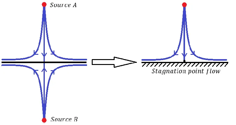
Figure 2.1: Combination of two flow sources

2.1.1

Leading-edge parabola

The shape of an airfoil can be given by the polynomial [1,2]:

𝑦 = ± 𝑇

_𝑜

𝑥

12

+ 𝐶

₁

𝑥 ± 𝑇

₁

𝑥

3

2

+ 𝐶

₂

𝑥

2

± 𝑇

₁

𝑥

5

2

..

(2.1)

where the coefficient series Ti represents the thickness and the coefficient series Ci represents the camber. The term x moves from the leading edge (usually at x = 0) to the trailing edge (usually at x = 1) along the chord. For a small value of x near the leading edge, (x < 5% chord) the terms with higher powers of x can be ignored leaving us with:

𝑦 = ± 𝑇

_𝑜

𝑥

12

+ 𝐶

₁

𝑥

(2.2)

In the above equation, the coefficient Todetermines the nose radius (r) of the airfoil and

the coefficient C1determines the initial slope (λ) of the camber line. We can rewrite equation

2.2 as:

10

Equation 2.3 represents an inclined parabola. Hence approximating the airfoil shape very close to the leading edge as a parabola is an acceptable assumption.

2.1.2

Potential flow and conformal mapping

Potential flow is defined as a flow that is incompressible (ρ = constant), irrotational (∇ 𝑋 𝑽 = 0) and isentropic. For such flows, the velocity potential (𝜑) and stream function (ψ) obey the Laplace equation. Since Laplace equation is linear, we can obtain a complex potential flow by superposing several elementary flows. Under these assumptions, the fluid velocity can be expressed as a gradient of the potential field, which is the objective of this section. Considering two analytical functions of z for complex potential (F) and complex velocity (W) given by:

𝐹(𝑧) = 𝜑(𝑧) + 𝑖 ψ(z)

(2.4)

𝑊(𝑧) = 𝐹′(𝑧) = 𝑢(𝑧) − 𝑖𝑣(𝑧)

(2.5)

where u and v are the x and y components of velocity respectively. The functions for F and W stated below can be used to represent simple flows such as uniform flow in an arbitrary direction, flow from a source or flow in a corner etc.

𝐹 =

𝐶

𝑛 + 1

𝑧

𝑛+1

_(2.6)

𝑊 = 𝐶𝑧

𝑛

(2.7)

where C is a complex number and n is an integer. For n = 1, we get the equations for stagnation-point flow shown in Figure 2.2 as follows:

𝐹(𝑧) =

𝐶

2

𝑧

2

₌

𝐶

2

(𝑥

2

_{− 𝑦}

2

_{) + 𝑖𝐶𝑥𝑦}

_(2.8)

11

Figure 2.2: Stagnation-point flow [1,2]

In certain cases, such as the flow over an airfoil, the complex shape of the airfoil makes it difficult to achieve proper visualization of the flow by simply superposing multiple elementary flows. In such cases, conformal mapping can be used to fully visualize the flow over such shapes. In conformal mapping, for each value of 𝑧 = 𝑥 + 𝑖𝑦 in the real plane, we have a corresponding value 𝜁 = 𝜉 + 𝑖𝜂 in the complex plane where 𝜉 = 𝜉(𝑥, 𝑦) and 𝜂 = 𝜂(𝑥, 𝑦). For the LEFS algorithm, the following complex potential mimics the stagnation flow discussed above [1,2]:

𝐹(𝜁) =

1

2

(𝜁 + 𝛽 − 1)

2

_(2.10)

which is of the form

𝐹(𝑧) =

𝐶

2

𝑧

2

_.

_{Hence the potential function can be used to represent}

stagnation-point flow which will be transformed to flow over the parabola by conformal mapping. This flow is mapped onto the z plane using the transformation function:

𝑧 =

1

2

(𝜁

12

Figure 2.3: Stagnation-point flow transformed to flow past a parabola [1,2]

Rearranging the terms of 𝐹′(𝜁) using substitutions 𝑌 = ±√2𝑋 where _{𝑋 = 𝑥 𝑟}⁄ , 𝑌 = 𝑦

𝑟

⁄ and 𝑦 = ±√2𝑟𝑥, we get the expression for velocity as:

𝑈

𝑈

_∞

=

𝐴(√𝑥 ± 𝑎

′

)

√𝑥 +

₂

𝑟

(2.12)

This expression is equal to the equation obtained by Van Dyke for the analytical solution for the flow past a parabola. Where 𝑎′= 𝛽√𝑟/2 and A is a multiplicative factor of order one. Using the value of velocity obtained from the above equation, we can calculate pressure coefficient using Bernoulli’s equation as follows:

𝑃 − 𝑃

_∞

=

1

2

𝜌𝑈

∞

2

_{[1 − (}

𝑈

𝑈

_∞

)

2

]

(2.13)

2.2

Methodology

13

discusses the nonlinear regression method and finally Subsection 2.2.4 discusses the procedure for generating the look-up tables and computing the final results.

2.2.1

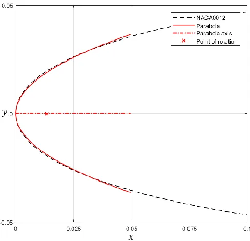
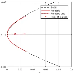
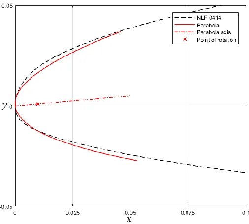
Parabola fitting

As discussed in Section 2.1.1 and 2.2.2, the airfoil shape very close to the leading edge can be approximated as a parabola. For the LEFS algorithm, a parabola fitting of up to 5% of the chord was opted. The parameters necessary to generate the parabola are the nose radius (r) and the initial slope of the camberline (λ). The first step is to calculate the parameter λ. This is done using an inviscid analysis in XFOIL. The airfoil coordinates are input into XFOIL and an inviscid sweep is carried out for small angles of attack between ±3 degrees with intervals of 0.1 degree. An algorithm computes the location of stagnation point for each angle of attack based on the direction of velocity (𝑈

𝑈∞) and gives out an ideal angle of attack (𝜃) at which the

stagnation point is at the leading edge (0,0) of the airfoil. The initial slope of the camberline is computed as:

𝜆 = tan (|𝜃|)

(2.14) The initial slope of the camberline and the airfoil coordinates are input into an algorithm that runs a least squares non-linear solver to compute the point of rotation for the parabola and the nose radius (r). The parameters r and 𝜆 form the basis for the parabola equation discussed in Section 2.1.1

𝑦 = ±√2𝑟𝑥 + 𝜆𝑥

(2.15)

For the case of a symmetric airfoil, the stagnation point is always at the leading edge of the airfoil hence the parameter

𝜆

becomes zero and the second term in equation 2.15 vanishes, leaving us with:

𝑦 = ±√2𝑟𝑥

(2.16)

14

Figure 2.4: Parabola fit for NACA0012

Figure 2.5: NACA0012

15

Figure 2.6: Parabola fit for S809

16

Figure 2.8: Parabola fit for NLF(1) - 0414

Figure 2.9: NLF(1) – 0414

2.2.2

Selection of pressure ports

For each airfoil, the location of pressure ports near the leading edge must be calibrated. For this algorithm, five pressure ports are used out of which the pressure data from three ports is used depending on the location of the stagnation point. It is important to properly calibrate the port locations to effectively capture the pressure readings. Once calibrated, the port locations for a specific airfoil can be used across all flap configurations and angles of attack.

17

compute the optimum pressure ports. In order to achieve this, the airfoil coordinates up to five percent of the chord are taken and split into multiple divisions depending on the level of accuracy desired. With the third pressure port fixed at the leading edge, the algorithm takes in different pressure values measured at two more distinct ports on the upper or lower surface depending on the location of the stagnation point. For every pressure port combination, the rms value of the difference between the actual and predicted velocities is computed. This value is compared against similar values for different pressure combination of port locations and the combination with the least rms value of difference is selected as the optimum location of pressure ports.

2.2.3

Non-linear regression

From the equation 2.13, substituting the value of 𝑈

𝑈∞ from equation 2.12, we have:

𝑃 − 𝑃

_∞

=

1

2

𝜌𝑈

∞

2

[

1 −

(

𝐴(√𝑥 ± 𝑎

′

)

√𝑥 +

𝑟

_{2 )}

2

]

(2.17)

Assuming

𝑃

_∞

, 𝜆, 𝑟

are known values, the pressure P can be represented as a function of

𝑈

_∞

, 𝑎, 𝐴

′and

𝑥

_𝑖

.

If

𝑃

_𝑖 is the pressure measured at pressure port i located at

𝑥

_𝑖, then the non-linear least squares optimizer (lsqnonlin) used in the algorithm seeks to minimize the value E given by:

𝐸 = ∑ 𝑒

_𝑖2

3

𝑖=1

(2.18)

18

stagnation point is on the upper surface, ports one, two and three are used. The algorithm continuously runs iterations using pressures at these 3 pressure ports till suitable values of

𝑎

′

, 𝐴

are found which minimizes E. The pressure distribution over a parabola calculated using equation 2.17 is compared with the pressures over an airfoil obtained using the XFOIL code in Figure 2.10. From the plots shown in Figure 2.10, we can see that the flow behavior over the parabola shows a good correlation with the flow over the airfoil in a region near the stagnation point.

Figure 2.10: A comparison of the XFOIL pressure distribution with the pressure distribution over the leading edge parabola for (a) S809 at an angle of attack of 5 degrees and (b)

NLF(1)-0414 at an angle of attack of 5 degrees

2.2.4

Computing results

A look-up table approach is used to interpolate between the values of

𝑎

′

, 𝐴

to compute

𝐶

_𝑙 and

19

The look-up table approach discussed above is common for airfoils with attached flaps as they can be directly analyzed in XFOIL. In case of multi-element airfoil, the pressure data was obtained from a series of CFD runs over a range of angles of attack. The obtained data was used as an input to the LEFS algorithm to generate the look-up tables. The entire LEFS procedure is summarized in Figure 2.11.

Figure 2.11: LEFS summary

20

Chapter 3

Simple flap airfoil analysis

This chapter presents the test results of the application of LEFS algorithm to different airfoils ranging from symmetric to highly cambered. As discussed in the previous chapters, the same leading-edge parabola and the pressure ports, as used by an unflapped airfoil, were used in case of corresponding airfoils with flaps extended. Every section discusses the entire procedure followed for an airfoil which includes the flap configurations tested, experimental test case setup (wind tunnel test data, CFD) and the air-data parameters computed by the LEFS algorithm. Section 3.1 discusses the result for S809 airfoil. Section 3.2 discusses the results for the natural laminar flow airfoils NLF(1)–0414 and NLF(1)–0215. Section 3.3 discusses the results for the NACA series airfoils NACA 0012 and NACA 23012.

3.1

NREL Wind tunnel: S809

21

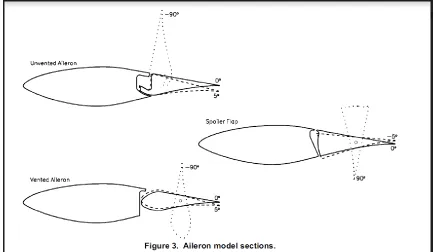
Figure 3.1: S809 flap/aileron configurations [22]

The wind tunnel tests were conducted at the OSU/AARL 7x10 subsonic wind tunnel [22,23] with an 18-inch constant chord NREL S809 airfoil shown in Figure 3.1. For this thesis, data for the cases of an unvented aileron at a Reynolds number of one million were selected. Each of the test cases had a 40% chord trailing-edge flap with deflections of -10, -5, 0, +5 degrees. The pressure port locations used for these airfoils is listed in Table 1. The look-up tables were generated using XFOIL at the given Reynolds number.

Table 1: Pressure port locations on the S809 airfoil S809 Pressure port locations (x/c)

Upper surface 0.025 0.005

Leading edge 0

Lower surface 0.01 0.03

22

23

24

Figure 3.4: Comparison of velocity, angle of attack and lift coefficient from LEFS and wind tunnel, for Re = 1 million with -10 degrees of flap

Comparing the results obtained by the algorithm with results from wind tunnel tests, LEFS can predict the air-data parameters accurately with very little error. The plots shown above, validate the applicability of the LEFS algorithm to the flapped S809 airfoil all the way up to stall.

3.2

Natural Laminar flow (NLF) Airfoils

25

3.2.1

NLF(1) - 0414

Figure 3.5: NLF(1) – 0414 airfoil with laminar flow up to x/c = 0.7

The NLF 0414 airfoil shown in Figure 3.5 is a 14% thick airfoil with a chord of 36 inches and a design lift coefficient of 0.4. It was designed for laminar flow up to 70% chord. The flap is hinged at [𝑥/𝑐, 𝑧/𝑐] = [0.875, −0.015]. The wind tunnel tests were conducted using a smooth airfoil at a Reynolds number of 3 million and a Mach number of 0.07 for the cases with flap angles 0, 5, 10 degrees and at a Reynolds number of 6 million and a Mach number of 0.07 for the cases with flap angles -5 and -10 [14]. The ports chosen to read the output pressure data from the wind tunnel tests are presented in Table 2.

Table 2: Pressure port locations on the NLF(1) - 0414 airfoil NLF(1) – 0414 Pressure port locations (x/c)

Upper surface 0.04 0.0052

Leading edge 0

Lower surface 0.0151 0.039

26

Figure 3.6: Comparison of velocity, lift coefficient and angle of attack from LEFS and wind tunnel, for Re = 3 million (a) NLF(1)-0414 with no flap (b) NLF(1)-0414 with 5 degrees of

27

Figure 3.7: Comparison of velocity, lift coefficient and angle of attack from LEFS and wind tunnel data (a) NLF(1)-0414 with 10 degrees of flap at a Re = 3 million (b) NLF(1)-0414

28

Figure 3.8: Comparison of velocity, lift coefficient and angle of attack from LEFS and wind tunnel data at Re = 6 million for NLF(1)-0414 with -10 degrees of flap

29

3.2.2

NLF(1) – 0215

Figure 3.9: NLF(1) – 0215 airfoil

The NLF(1) - 0215 airfoil shown in Figure 3.9 is a 15% thick airfoil with a chord of 24 inches and a design lift coefficient of 0.2. It was designed to achieve a primary goal of reducing wing parasite drag. The wind tunnel tests were conducted using a smooth airfoil at a Reynolds number of 6 million and a Mach number of 0.1. The airfoil comes with a flap hinged at

[𝑥/𝑐, 𝑧/𝑐] = [0.75, 0.0328] which is deflected 10 and -10 degrees for the experiment. The low drag region or the drag bucket can be moved down or up relative to the lift coefficient by moving the flap up or down respectively. The ports chosen to read the output pressure data from the wind tunnel tests are presented in Table 3.

Table 3: Pressure port locations on the NLF(1) - 0215 airfoil NLF(1) – 0215 Pressure port locations (x/c)

Upper surface 0.0254 0.0057

Leading edge 0

Lower surface 0.01 0.04

30

Figure 3.10: Comparison of velocity, lift coefficient and angle of attack from LEFS and wind tunnel data at a Re = 6 million for (a) NLF(1)-0215 with no flap and (b) NLF(1)-0215 with

31

Figure 3.11: Comparison of velocity, lift coefficient and angle of attack from LEFS and wind tunnel data at Re = 6 million for NLF(1)-0215 with -10 degrees of flap

32

3.3

NACA Airfoil Series

This section presents the application of the LEFS algorithm to flapped cases of the symmetric airfoil NACA 0012 and cambered airfoil NACA 23012. The pressure data for each of the airfoils was obtained by CFD analysis. For each airfoil, the flap angles analyzed are 0, +5, +10 and -5.

3.3.1

Meshing

The airfoils were meshed using a 2-D structured O-grid mesh. The mesh was split into two regions, the outer and inner. The boundaries of the meshed region were open and were twenty chord lengths away in all directions. The front, top and bottom boundaries were subject to the velocity inlet boundary condition while the rear boundary was subject to the pressure outlet boundary condition. The entire meshed region was split into two parts. The outer region was made of medium to coarse cells as they only capture the freestream inlet/outlet flow. The inner region which was in proximity to the airfoil was made of fine elements consisting of 300,000 elements. Across all regions, the number of elements totaled to 500,000 with a mesh quality of 0.97. The fluid properties used for the CFD analysis are given in Table 4.

Table 4: Properties of air

Re 3 million ρ (Kg/m3_{) 1.225} μ (Nsec/m2_{) 1.84e-5}

T (K) 288.16

Based on the above properties, for a chord of one meter, using equation 3.1 the freestream velocity is computed to be 43.82 m/s.

𝑅𝑒 =

𝜌 . 𝑈

∞

. 𝑐

33

Using the Reynolds number and the value of freestream velocity, the minimum element size or the wall distance in the inflation layer which is important to capture the boundary layer can be computed. Using the Schlichting skin-friction correlation we have:

𝐶

_𝑓

= [2 log

₁₀

(𝑅𝑒

_𝑥

) − 0.65]

−2.3

_(3.2)

Substituting the skin friction coefficient in equation 3.3 to compute wall shear stress

(𝜏

_𝜔

)

𝜏

_𝜔

= 𝐶

_𝑓

.

1

2

𝜌𝑈

2

∞

(3.3)

Substituting wall sheer stress in equation 3.4 to compute friction velocity

𝑢

_∗

= √

𝜏

𝜔

𝜌

(3.4)

For

𝑦

+

= 1

,

we compute the wall distance (y) as follows

𝑦 =

𝑦

+

_𝜇

𝑢

_∗

= 0.0000085

(3.5)

Figure 3.12 shows the inflation layer used for capturing the boundary layer while Figure 3.13 shows two cases of the meshed NACA 0012 and the NACA 23012 airfoils.

34

Figure 3.13: (a) NACA 0012 airfoil with 5 degrees of flap (b) NACA 23012 with 5 degrees of flap

3.3.2

CFD

35

Figure 3.14: Cp plots from CFD results at 𝛼 = 0 (a) NACA 0012 airfoil with 5 degrees of flap (b) NACA 0012 airfoil with 10 degrees of flap (c) NACA 0012 airfoil with -5 degrees of

36

3.3.3

NACA 0012

Figure 3.15: NACA 0012 airfoil

The airfoil coordinates were obtained using the online NACA airfoil generator. The NACA-0012 airfoil shown in Figure 3.15 was generated with a closed trailing edge for easier meshing. The flap configurations of +5, +10 and -5 were hinged at [𝑥/𝑐, 𝑧/𝑐] = [0.80, 0.00]. The base airfoil coordinates were input to XFOIL and the flaps were set at the selected hinge point using the geometry design routine option. The pressure ports use for the analysis are given in Table 5.

Table 5: Pressure port locations on the NACA 0012 airfoil NACA 0012 Pressure port locations (x/c)

Upper surface 0.05 0.0052

Leading edge 0

Lower surface 0.02 0.04

37

Figure 3.16: Comparison of velocity, lift coefficient and angle of attack from LEFS and CFD results at a Re = 3 million for (a) NACA 0012 with no flap and (b) NACA 0012 with 5

38

Figure 3.17: Comparison of velocity, lift coefficient and angle of attack from LEFS and CFD results at a Re = 3 million for (a) NACA 0012 with 10 degrees of flap and (b) NACA 0012

39

Comparing the results shown above, it can be concluded that all the air-data parameters are predicted accurately with very little error. Hence the applicability of the LEFS algorithm to the flapped cases of the NACA 0012 airfoil all the way up to stall is validated.

3.3.4

NACA 23012

Figure 3.18: NACA 23012 airfoil

Similar to the NACA 0012, the airfoil coordinates for NACA 23012 were obtained using the online NACA airfoil generator. The airfoil shown in figure 3.18 was generated with a closed trailing edge for easier meshing. The flap configurations of +5, +10 and -5 were hinged at

[𝑥/𝑐, 𝑧/𝑐] = [0.80, 0.00]. The base airfoil coordinates were input to XFOIL and the flaps were set at the selected hinge point using the geometry design routine option. The pressure ports used for this airfoil are presented in Table 6 below:

Table 6: Pressure port locations on the NACA 23012 airfoil NACA 23012 Pressure port locations (x/c)

Upper surface 0.045 0.012

Leading edge 0

Lower surface 0.005 0.01

40

Figure 3.19: Comparison of velocity, lift coefficient and angle of attack from LEFS and CFD results at a Re = 3 million for (a) NACA 23012 with no flap and (b) NACA 23012 with 5

41

Figure 3.20: Comparison of velocity, lift coefficient and angle of attack from LEFS and CFD results at a Re = 3 million for (a) NACA 23012 with 10 degrees of flap and (b) NACA 23012

42

43

Chapter 4

Multi-element airfoil analysis

This chapter presents the test results of the application of LEFS algorithm to multi-element airfoils where the flap is a separate element from the main airfoil. This airfoil configuration is commonly found on most commercial aircrafts. Figure 4.1 shows double and triple slotted flaps.

44

The airfoil analyzed in this chapter is the two-element UIUC1600 [24,25] and is shown in Figure 4.2. The flap (shown in Figure 4.3) was deflected to an angle (δ) of 36o_{. The airfoil} is typical of wings found on open wheel racecars.

Figure 4.2: UIUC 1600 two element airfoil

Figure 4.3: flap angle The airfoil parameters are shown in Table 7.

Table 7: Airfoil Parameters Parameter Value Main Element Chord (c1) 1m

45

The analysis of this airfoil has been carried out using the LEFS algorithm for two cases: The entire configuration and separately for the flap element. In the analysis of the entire airfoil, the pressures measured at the ports on the leading edge of the main element were used to compute the angle of attack, lift coefficient and freestream velocity. On the other hand, for the analysis of flow over the flap, five pressure ports are fit on the leading edge of the flap element and the pressures measured are used to compute only the lift coefficient. Computing angle of attack and freestream velocity is not possible using the algorithm as the flow over the flap is influenced by the main element. The airfoil was meshed using ANSYS Workbench meshing tool and the pressure data was obtained from CFD results.

In this chapter, Section 4.1 discusses the procedure followed for meshing the airfoil. Section 4.2 discusses the CFD case setup procedure. Section 4.3 and Section 4.4 discuss the results for analysis of the entire airfoil and the flap element respectively.

4.1

Meshing

The airfoil was meshed using ANSYS Workbench. In the design modeler tool, the main and flap elements were imported as separate bodies and were given unique named selections. This enabled the measurement of lift coefficient exclusively on the flap element. The boundaries of the meshed region were modelled twenty chord lengths (based on the chord of the main element) away in all directions. The front, top and bottom boundaries were subject to the velocity inlet boundary condition while the rear boundary was subject to the pressure outlet boundary condition.

46

Figure 4.4: Meshed UIUC 1600

Figure 4.5: Inflation layers on main and flap element

4.2

CFD

47

Table 8: CFD parameters

Re 3e6

U∞ (m/s) 32.567 ρ (Kg/m3_{) 1.225} μ (Nsec/m2_{) 1.84e-5}

T (K) 288.16

Since the main and flap elements have separate named selections, for the analysis of the entire airfoil, the lift coefficient data was monitored by selecting both the surfaces with wall boundary condition. Pressure data was obtained over a range of angles of attack from -12 degrees to 10 degrees. The pressure data was used as an input to run the LEFS algorithm to set up the look-up tables.

For analysis of flap element, the lift was measured exclusively on the flap. The CFD analysis had to be carried out for the entire airfoil configuration as the flow over the flap is influenced by the main element. Figures 4.6, 4.7 and 4.8 show the CFD results for UIUC 1600.

48

Figure 4.7: CP distribution from CFD results at 𝛼 = 0

49

4.3

Results

For the analysis of the entire airfoil, the five pressure ports chosen on the leading edge are shown in Table 9. The look-up tables were generated by obtaining pressure data over a range of angles of attack from CFD analysis.

Table 9: main element pressure ports Pressure port locations (x/c)

Upper surface 0.025 0.005

Leading edge 0

Lower surface 0.035 0.05

50

Figure 4.9: Comparison of velocity, lift coefficient and angle of attack from LEFS and CFD data at Re = 3 million for the multielement airfoil UIUC 1600

For the analysis of the flap element, the flap coordinates were rotated such that the chord lies on the x-axis. The parabola was fit to the flap element in this configuration using the procedure discussed in Section 2.2.1. The pressure port locations for the rotated flap are shown in Table 10.

Table 10: Pressure port locations for rotated flap coordinates with chord along x-axis Pressure port locations (X/c) for rotated flap

Upper surface 0.025 0.005

Leading edge 0

51

The coordinates were then rotated back to the original flap configuration using equation 4.1. The corresponding y-coordinates were obtained using MATLAB

𝑥 = 𝑋 ∗ 0.4517 + 0.9414

4.1

The pressure ports on the flap are shown in Table 11.

Table 11: Pressure port locations on flap element Flap element pressure port locations (x/c)

Upper surface 0.953 0.944 Leading edge 0.9414 Lower surface 0.957

0.964

The predicted lift coefficient values for the flap are shown in Figure 4.10

Figure 4.10: Comparison of lift coefficient from LEFS and CFD data at Re = 3 million for the flap element of UIUC 1600

52

53

Chapter 5

Conclusions

Tracking air-data parameters on a real-time basis can significantly reduce the risk of running into dangerous stall situations. The LEFS algorithm presented by Saini et al [1,2] has been tested to work on an unflapped airfoil. The algorithm can successfully predict the freestream velocity, lift coefficient and angle of attack on a wing section and can be extended to separately compute the parameters for different sections of the wing.

An aircraft uses flaps to generate higher lift at lower speeds especially during takeoffs and landings. Most cases of aircraft stall have occurred during takeoff or landing hence the algorithm must be capable of computing the air-data parameters of airfoils with the flaps extended as well. The work presented in this thesis successfully extended the application of the LEFS algorithm to cases with flaps extended. The applicability has been verified by testing several airfoils with different flap angles. In all the cases, the LEFS algorithm successfully predicted the parameters with a small percentage of error (less than 8%). Multi-element airfoils are commonly found on most commercial aircraft. The LEFS algorithm was also tested on the multi-element UIUC 1600 airfoil with flap element deflected to 36 degrees which is close to the maximum flap deflection used by commercial aircraft during landing. The algorithm successfully predicted the air-data parameters leading up to stall.

54

National Renewable Energy Laboratory has explored the applicability of aileron devices on horizontal axis wind turbines for speed control, power modulation and aerodynamic braking. For this test, the S809 airfoil with different aileron configurations were used. This thesis has also successfully verified the applicability of LEFS algorithm to the above-mentioned cases. Real-time analysis of airfoil performance data will not only help monitor and diagnose problems but will also be useful for future wind turbine design.

5.1

Future work

In the case of the multi-element airfoil, CFD analysis of the flap element was done using ANSYS FLUENT and the pressure data at the five pressure port locations on the leading edge of the flap was extracted. This data was used to run the LEFS algorithm for various angles of attack. The values of lift coefficient predicted by the algorithm showed good correlation with the CFD results. This process can be replicated with double, triple or multi slotted flaps to analyze each element separately. The predicted value of lift coefficient using LEFS could be used to determine the optimum flap position for maximum lift.

Further, different cases of leading-edge lift enhancing devices such as slats could be explored. Figure 5.1 shows a few such devices. Figure 5.2 shows the leading-edge slats on the Boeing 737.

55

Figure 5.2: Leading edge slats on the Boeing 737. Image source: https://history.nasa.gov/SP-468/ch10-5.htm

56

REFERENCES

[1] Dr. Aditya Saini (2017) Leading edge flow sensing for aerodynamic parameter estimation. Doctoral Dissertation, Department of Mechanical and Aerospace Engineering. North Carolina State University

[2] Saini, Aditya & Gopalarathnam, Ashok. (2018). Leading-Edge Flow Sensing for Aerodynamic Parameter Estimation. AIAA Journal. 56. 1-13. 10.2514/1.J057327. [3] Sofia Larsson Cahlin (2016) Real time estimation of aerodynamic parameters.

Division of automatic control, department of electrical engineering, Linkoping University, SE-581 83Linkoping Sweden.

[4] Liu, Hao & Ravi, Sridhar & Kolomenskiy, Dmitry & Tanaka, Hiroto. (2016). Biomechanics and biomimetics in insect-inspired flight systems. Philosophical Transactions of the Royal Society B. 371. 10.1098/rstb.2015.0390.

[5] Shyy, Wei & Kang, Chang-kwon & Chirarattananon, Pakpong & Ravi, Sridhar & Liu, Hao. (2016). Aerodynamics, sensing and control of insect-scale flapping-wing flight. Proceedings of the Royal Society A: Mathematical, Physical and Engineering Science. 472. 20150712. 10.1098/rspa.2015.0712.

[6] E Brown, Richard & Roger Fedde, M. (1993). Airflow sensors in the avian wing. J. Exp. Biol.. 179.

[7] Brücker, C. , Schlegel, D. and Triep, M. (2016) Feather Vibration as a Stimulus for Sensing Incipient Separation in Falcon Diving Flight. Natural Resources, 7, 411-422. doi: 10.4236/nr.2016.77036

[8] Fang, Z. Aircraft Flight Dynamics and Automatic Flight Control; National Defense Industry Press: Beijing, China, 1999

[9] Hagen, F.W.; Seidel, H. Deutsche airbus flight test of rosemount smart probe for distributed air data systems. IEEE AES Syst. Mag. 1994, 9, 7–14

[10] Callegari, S.; Talamelli, A.; Zagnoni, M.; Golfarelli, A.; Rossi, V.; Tartagni, M.; Sangiorgi, E. Aircraft angle of attack and air speed detection by redundant strip pressure sensors. Proc. IEEE 2004, 3, 1526–1529

[11] Que, Ruiyi & Zhu, Rong. (2012). Aircraft Aerodynamic Parameter Detection Using Micro Hot-Film Flow Sensor Array and BP Neural Network Identification. Sensors (Basel, Switzerland). 12. 10920-9. 10.3390/s120810920.

57

[13] Srivastava, Ankur & Meade, Andrew & Long, Kurtis. (2012). Learning Air-Data Parameters for Flush Air Data Sensing Systems. Journal of Aerospace Computing, Information, and Communication. 9. 10.2514/1.54947.

[14] Robert J. McGhee, Jeffery K. Viken, Werner Pfenninger, William D. Beasley & William D. Harvey (1984) Experimental results for a flapped natural laminar flow airfoil with high lift/drag ratio (NASA). HC A14/MF A01

[15] Que, R.Y.; Zhu, R.; Wei, Q.Z.; Cao, Z. A Flexible Integrated Micromachined Hot-film Sensor array for Measuring Surface Flow Vector. In Proceedings of the 16th International Conference on Solid-State Sensors, Actuators and Microsystems, Beijing, China, 5–9 June 2011; pp. 108–111.

[16] Thomas P Webb, Richard J Prazenica, Andrew J Kurdila, and Rick Lind. Vision-based state estimation for autonomous micro air vehicles. Journal of guidance, control, and dynamics, 30(3):816{826, 2007.

[17] Scott M Ettinger, Michael C Nechyba, Peter G Ifju, and Martin Waszak. Vision-guided fight stability and control for micro air vehicles. Advanced Robotics, 17(7):617{640, 2003}.

[18] Takeo Kanade, Omead Amidi, and Qifa Ke. Real-time and 3d vision for autonomous small and micro air vehicles. In 43rd IEEE Conference on Decision and Control (CDC 2004), December 2004.

[19] R. Reuss Ramsay, M.J. Hoffmann, and G.M. Gregorek. Effects of Grit Roughness and Pitch Oscillations on the S809 Airfoil. NREL/TP 442, 1995.

[20] Wang, Qing & Chen, Yan & Tang, Hui. (2012). Mechanism Design for Aircraft Morphing Wing. 53rd AIAA/ASME/ASCE/AHS/ASC Structures, Structural Dynamics and Materials Conference 2012. 10.2514/6.2012-1608.

[21] Bashir, M., Rajendran, P., & Mule, A. (2018). Investigation on Three-Dimensional CFD Validation for a Variable Span Morphing Wing. Asian Journal For Convergence In Technology (AJCT), 3(3).

[22] R.R.Ramsey, J.M.Janiszewska, G.M.Gregorek (1996) Wind Tunnel Testing of Three S809 Aileron Configurations for use on Horizontal Axis Wind Turbines. Ohio state University

58

[24] Carroll, C (2005) High Downforce Airfoils in Ground Effect: A Trade Study for Use in Open-Wheeled Racecar Front-Wing Design. Master’s thesis, Department of Aerospace Engineering, University of Illinois at Urbana-Champaign, Urbana, IL 61801, USA

59

60

Appendix

Airfoil Coordinates

A.1 S809

1.000000 0.001149 0.997537 0.002242 0.992905 0.003175 0.986862 0.004216 0.978984 0.005531 0.968840 0.007319 0.956612 0.009559 0.943049 0.012108 0.928875 0.014753 0.914449 0.017454 0.899964 0.020143 0.885411 0.022812 0.870864 0.025497 0.856346 0.028169 0.841796 0.030823 0.827240 0.033501 0.812721 0.036198 0.798209 0.038906 0.783669 0.041623 0.769110 0.044371 0.754539 0.047138 0.739984 0.049903 0.725443 0.052639 0.710883 0.055401

61 0.325005 0.097839

0.310678 0.096821 0.296371 0.095618 0.282101 0.094237 0.267837 0.092661 0.253572 0.090913 0.239321 0.088990 0.225108 0.086912 0.210951 0.084648 0.196844 0.082221 0.182831 0.079594 0.168915 0.076759 0.155034 0.073717 0.141332 0.070442 0.127629 0.066912 0.114158 0.063243 0.101122 0.059365 0.088665 0.055341 0.077351 0.051376 0.067809 0.047778 0.060241 0.044701 0.054280 0.042175 0.049727 0.040181 0.045963 0.038516 0.042793 0.036964 0.040026 0.035611 0.037545 0.034352 0.035285 0.033162 0.033158 0.032035 0.031094 0.030881 0.029074 0.029744 0.027061 0.028524 0.025026 0.027246 0.022955 0.025933 0.020859 0.024537 0.018717 0.023057 0.016560 0.021442 0.014387 0.019751 0.012248 0.017987 0.010185 0.016211 0.008293 0.014391 0.006497 0.012508 0.004755 0.010472 0.003106 0.008269 0.001646 0.005826 0.000500 0.003124

62 0.233168 -0.093973

0.247073 -0.096702 0.260987 -0.099156 0.274941 -0.101361 0.288922 -0.103327 0.302839 -0.105008 0.316820 -0.106398 0.330730 -0.107526 0.344628 -0.108301 0.358530 -0.108774 0.372352 -0.108932 0.386115 -0.108693 0.399914 -0.108104 0.413673 -0.107159 0.427459 -0.105853 0.441219 -0.104223 0.454981 -0.102242 0.468741 -0.099947 0.482524 -0.097333 0.496366 -0.094427 0.510310 -0.091271 0.524326 -0.087913 0.538451 -0.084405 0.552627 -0.080779 0.566824 -0.077082 0.581079 -0.073310 0.595361 -0.069511 0.609669 -0.065709 0.623940 -0.061907 0.638207 -0.058123 0.652490 -0.054366 0.666771 -0.050660 0.681062 -0.046992 0.695296 -0.043377 0.709485 -0.039873 0.723683 -0.036478 0.737917 -0.033137 0.752112 -0.029895 0.766283 -0.026779 0.780474 -0.023804 0.794696 -0.020963 0.808920 -0.018223 0.823028 -0.015677 0.837201 -0.013336 0.851402 -0.011139 0.865511 -0.009115

63

A.2 NLF(1)-0414

1.0000000000 -0.0271220000 0.9994800000 -0.0270670000 0.9979520000 -0.0268720000 0.9954560000 -0.0265190000 0.9920210000 -0.0260060000 0.9876600000 -0.0253330000 0.9823700000 -0.0244920000 0.9761550000 -0.0234560000 0.9690340000 -0.0222060000 0.9610420000 -0.0207220000 0.9522000000 -0.0189940000 0.9425110000 -0.0170080000 0.9319800000 -0.0147390000 0.9206590000 -0.0121610000 0.9086440000 -0.0092670000 0.8960060000 -0.0060440000 0.8827680000 -0.0024750000 0.8689600000 0.0014670000 0.8546930000 0.0057930000 0.8400760000 0.0104640000 0.8251790000 0.0154830000 0.8101240000 0.0207500000 0.7950340000 0.0261780000 0.7799510000 0.0316940000 0.7649250000 0.0372080000 0.7500580000 0.0425420000 0.7353920000 0.0474920000 0.7207510000 0.0519440000 0.7058600000 0.0558890000 0.6905860000 0.0593760000 0.6749260000 0.0625100000 0.6589280000 0.0653480000 0.6426290000 0.0679000000 0.6260400000 0.0702450000 0.6091770000 0.0723770000 0.5920640000 0.0742850000 0.5747420000 0.0759880000 0.5572540000 0.0774890000 0.5396410000 0.0787790000 0.5219310000 0.0798930000 0.5041590000 0.0807940000 0.4863270000 0.0815070000

64 0.0000850000 -0.0015350000

0.0001640000 -0.0021200000 0.0007400000 -0.0045360000 0.0020950000 -0.0069840000 0.0041740000 -0.0090080000 0.0071290000 -0.0109930000 0.0108740000 -0.0129330000 0.0155400000 -0.0148820000 0.0210960000 -0.0168540000 0.0273800000 -0.0187970000 0.0345690000 -0.0207420000 0.0423930000 -0.0226540000 0.0509850000 -0.0245720000 0.0602740000 -0.0264870000 0.0702430000 -0.0283830000 0.0808810000 -0.0302590000 0.0921590000 -0.0321160000 0.1040580000 -0.0339450000 0.1165570000 -0.0357410000 0.1296350000 -0.0374970000 0.1432770000 -0.0392120000 0.1574570000 -0.0408880000 0.1721480000 -0.0425210000 0.1873280000 -0.0441070000 0.2029690000 -0.0456460000 0.2190430000 -0.0471250000 0.2355250000 -0.0485420000 0.2523870000 -0.0499010000 0.2695860000 -0.0511890000 0.2870670000 -0.0524110000 0.3048660000 -0.0535610000 0.3229010000 -0.0546315000 0.3411560000 -0.0556350000 0.3596110000 -0.0565390000 0.3762600000 -0.0573440000 0.3970740000 -0.0580520000 0.4160170000 -0.0586580000 0.4350490000 -0.0591420000 0.4541270000 -0.0595170000 0.4732220000 -0.0597850000 0.4923190000 -0.0599500000 0.5114020000 -0.0600120000 0.5304300000 -0.0599790000 0.5493610000 -0.0597920000 0.5681600000 -0.0594560000 0.5867620000 -0.0589820000

65

A.3 NLF(1)-0215

1.000000 0.000000 0.995504 0.001673 0.987975 0.004708 0.979507 0.008187 0.970591 0.011677 0.961279 0.015003 0.951376 0.018224 0.940792 0.021383 0.929554 0.024522 0.917791 0.027668 0.905674 0.030800 0.893326 0.033907 0.880808 0.036986 0.868163 0.040035 0.855429 0.043054 0.842631 0.046042 0.829788 0.048997 0.816909 0.051921 0.804000 0.054814 0.791070 0.057678 0.778129 0.060511 0.765187 0.063309 0.752246 0.066072 0.739305 0.068799 0.726361 0.071488 0.713415 0.074141 0.700469 0.076755 0.687532 0.079329 0.674609 0.081857 0.661706 0.084336 0.648823 0.086763 0.635963 0.089134 0.623126 0.091445 0.610317 0.093693 0.597537 0.095871 0.584795 0.097974 0.572102 0.099993 0.559476 0.101919 0.546937 0.103741 0.534497 0.105444 0.522159 0.107015 0.509911 0.108446 0.497736 0.109728 0.485616 0.110860

66 0.018187 0.028694

0.015177 0.025961 0.012599 0.023404 0.010376 0.020984 0.008443 0.018670 0.006757 0.016442 0.005293 0.014299 0.004037 0.012250 0.002971 0.010310 0.002075 0.008483 0.001341 0.006769 0.000771 0.005153 0.000359 0.003614 0.000101 0.002126 0.000000 0.000000 0.000049 -0.000779 0.000267 -0.002226 0.000653 -0.003662 0.001221 -0.005069 0.001995 -0.006421 0.003007 -0.007677 0.004284 -0.008816 0.005844 -0.009850 0.007701 -0.010798 0.009867 -0.011693 0.012324 -0.012587 0.015072 -0.013517 0.018161 -0.014480 0.021643 -0.015469 0.025585 -0.016479 0.030099 -0.017514 0.035353 -0.018586 0.041545 -0.019704 0.048870 -0.020883 0.057417 -0.022119 0.067061 -0.023360 0.077531 -0.024556 0.088689 -0.025690 0.100440 -0.026753 0.112638 -0.027744 0.125129 -0.028657 0.137791 -0.029493 0.150565 -0.030257 0.163434 -0.030955 0.176380 -0.031590 0.189385 -0.032169

67 0.787466 0.004685

68

A.4 NACA 0012 (Closed trailing edge)

1.000000 0.000000 0.999753 0.000036 0.999013 0.000143 0.997781 0.000322 0.996057 0.000572 0.993844 0.000891 0.991144 0.001280 0.987958 0.001737 0.984292 0.002260 0.980147 0.002849 0.975528 0.003501 0.970440 0.004216 0.964888 0.004990 0.958877 0.005822 0.952414 0.006710 0.945503 0.007651 0.938153 0.008643 0.930371 0.009684 0.922164 0.010770 0.913540 0.011900 0.904508 0.013071 0.895078 0.014280 0.885257 0.015523 0.875056 0.016800 0.864484 0.018106 0.853553 0.019438 0.842274 0.020795 0.830656 0.022173 0.818712 0.023569 0.806454 0.024981 0.793893 0.026405 0.781042 0.027838 0.767913 0.029279 0.754521 0.030723 0.740877 0.032168 0.726995 0.033610 0.712890 0.035048 0.698574 0.036478 0.684062 0.037896 0.669369 0.039300 0.654508 0.040686 0.639496 0.042052 0.624345 0.043394 0.609072 0.044708

69 0.035112 0.030473

70 0.904508 -0.013071

71

A.5 NACA 23012 (Closed trailing edge)

1.000000 -0.000000 0.990032 0.001665 0.980063 0.003311 0.970094 0.004939 0.960125 0.006549 0.950155 0.008142 0.940185 0.009718 0.930215 0.011276 0.920244 0.012819 0.910273 0.014345 0.900301 0.015856 0.890330 0.017350 0.880357 0.018829 0.870385 0.020293 0.860412 0.021742 0.850439 0.023176 0.840465 0.024595 0.830491 0.025999 0.820517 0.027389 0.810543 0.028764 0.800568 0.030126 0.790593 0.031472 0.780617 0.032805 0.770641 0.034124 0.760665 0.035428 0.750689 0.036718 0.740712 0.037994 0.730735 0.039255 0.720758 0.040502 0.710780 0.041735 0.700802 0.042953 0.690824 0.044156 0.680845 0.045345 0.670866 0.046518 0.660887 0.047677 0.650907 0.048819 0.640927 0.049947 0.630947 0.051058 0.620966 0.052153 0.610985 0.053231 0.601004 0.054293 0.591022 0.055337 0.581040 0.056364 0.571057 0.057373

72 0.118394 0.067796

73 0.799432 -0.021292