Simple Penalties on Maximum-Likelihood Estimates of Genetic Parameters to Reduce Sampling Variation

| INVESTIGATION

Simple Penalties on Maximum-Likelihood Estimates

of Genetic Parameters to Reduce Sampling Variation

Karin Meyer1

Animal Genetics and Breeding Unit, University of New England, Armidale, New South Wales 2351, Australia ORCID ID: 0000-0003-2663-9059 (K.M.)

ABSTRACTMultivariate estimates of genetic parameters are subject to substantial sampling variation, especially for smaller data sets

and more than a few traits. A simple modification of standard, maximum-likelihood procedures for multivariate analyses to estimate genetic covariances is described, which can improve estimates by substantially reducing their sampling variances. This is achieved by maximizing the likelihood subject to a penalty. Borrowing from Bayesian principles, we propose a mild, default penalty—derived assuming a Beta distribution of scale-free functions of the covariance components to be estimated—rather than laboriously attempting to determine the stringency of penalization from the data. An extensive simulation study is presented, demonstrating that such penalties can yield very worthwhile reductions in loss,i.e., the difference from population values, for a wide range of scenarios and without distorting estimates of phenotypic covariances. Moreover, mild default penalties tend not to increase loss in difficult cases and, on average, achieve reductions in loss of similar magnitude to computationally demanding schemes to optimize the degree of penalization. Pertinent details required for the adaptation of standard algorithms to locate the maximum of the likelihood function are outlined.

KEYWORDSgenetic parameters; improved estimates; regularization; maximum likelihood; penalty

E

STIMATION of genetic parameters,i.e., partitioning of phenotypic variation into its causal components, is one of the fundamental tasks in quantitative genetics. For multi-ple characteristics of interest, this involves estimation of co-variance matrices due to genetic, residual, and possibly other random effects. It is well known that such estimates can be subject to substantial sampling variation. This holds espe-cially for analyses comprising more than a few traits, as the number of parameters to be estimated increases quadrati-cally with the number of traits considered, unless the covari-ance matrices of interest have a special structure and can be modeled more parsimoniously. Indeed, a sobering but realis-tic view is that“Few datasets, whether from livestock, labo-ratory or natural populations, are of sufficient size to obtain useful estimates of many genetic parameters”(Hill 2010, p. 75). This not only emphasizes the importance of appropriate

data, but also implies that a judicious choice of methodology for estimation—which makes the most of limited and pre-cious records available—is paramount.

A measure of the quality of an estimator is its“loss,”i.e., the deviation of the estimate from the true value. This is an ag-gregate of bias and sampling variation. We speak of improv-ing an estimator if we can modify it so that the expected loss is lessened. In most cases, this involves reducing sampling variance at the expense of some bias—if the additional bias is small and the reduction in variance sufficiently large, the loss is reduced. In statistical parlance“regularization”refers to the use of some kind of additional information in an anal-ysis. This is often used to solve ill-posed problems or to pre-vent overfitting through some form of penalty for model complexity; see Bickel and Li (2006) for a review. There has been longstanding interest, dating back to Stein (1975) and earlier (James and Stein 1961), in regularized estimation of covariance matrices to reduce their loss. Recently, as esti-mation of higher-dimensional matrices is becoming more ubiquitous, there has been a resurgence in interest (e.g., Bickel and Levina 2008; Warton 2008; Witten and Tibshirani 2009; Ye and Wang 2009; Rothmanet al.2010; Fisher and Sun 2011; Ledoit and Wolf 2012; Deng and Tsui 2013; Won

Copyright © 2016 by the Genetics Society of America doi: 10.1534/genetics.115.186114

Manuscript received December 14, 2015; accepted for publication June 9, 2016; published Early Online June 13, 2016.

Supplemental material is available online atwww.genetics.org/lookup/suppl/doi:10. 1534/genetics.115.186114/-/DC1.

1_{Address for correspondence: Animal Genetics and Breeding Unit, University of New}

et al.2013). In particular, estimation encouraging sparsity is an activefield of research for estimation of covariance matri-ces (e.g., Pourahmadi 2013) and in related areas, such as graphical models and structural equations.

Improving Estimates of Genetic Parameters

As emphasized above, quantitative genetic analyses require at least two covariance matrices to be estimated, namely due to additive genetic and residual effects. The partitioning of the total variation into its components creates substantial sam-pling correlations between them and tends to exacerbate the effects of sampling variation inherent in estimation of co-variance matrices. However, most studies on regularization of multivariate analyses considered a single covariance matrix only and the literature on regularized estimates of more than one covariance matrix is sparse. In a classic article, Hayes and Hill (1981) proposed to modify estimates of the genetic co-variance matrixðSGÞby shrinking the canonical eigenvalues

of SG and the phenotypic covariance matrix ðSPÞ toward

their mean, a procedure described as“bending”the estimate ofSGtoward that ofSP:The underlying rationale was that

SP;the sum of all the causal components, is typically

esti-mated much more accurately than any of its components, so that bending would“borrow strength”from the estimate of

SP;while shrinking estimated eigenvalues toward their mean

would counteract their known, systematic overdispersion. The authors demonstrated by simulation that use of “bent” estimates in constructing selection indexes could increase the achieved response to selection markedly, as these were closer to the population values than unmodified estimates and thus provided more appropriate estimates of index weights. How-ever, no clear guidelines to determine the optimal amount of shrinkage to use were available and bending was thus pri-marily used only to modify nonpositive definite estimates of covariance matrices and all but forgotten when methods that allowed estimates to be constrained to the parameter space became common procedures.

Modern analyses to estimate genetic parameters are gen-erally carried out fitting a linear mixed model and using restricted maximum-likelihood (REML) or Bayesian method-ology. The Bayesian framework directly offers the opportunity for regularization through the choice of appropriate priors. Yet, this is rarely exploited for this purpose and “flat” or minimally informative priors are often used instead (Thompson et al.2005). In a maximum-likelihood context, estimates can be regularized by imposing a penalty on the likelihood function aimed at reducing their sampling vari-ance. This provides a direct link to Bayesian estimation: For a given prior distribution of the parameters of interest or functions thereof, an appropriate penalty can be obtained as a multiple of minus the logarithmic value of the probability density function. For instance, shrinkage of eigenvalues to-ward their mean through a quadratic penalty on the likeli-hood is equivalent to assuming a normal distribution of the eigenvalues while the assumption of a double exponential

prior distribution results in a LASSO-type penalty (Huang

et al.2006).

Meyer and Kirkpatrick (2010) demonstrated that a REML analog to bending is obtained by imposing a penalty propor-tional to the variance of the canonical eigenvalues on the likelihood and showed that this can yield substantial reduc-tions in loss for estimates of both SG andSE;the residual

covariance matrix. Subsequent simulations (Meyer et al.

2011; Meyer 2011) examined the scope for penalties based on different functions of the parameters to be estimated and prior distributions for them and found them to be similarly effective, depending on the population values for the covari-ance matrices to be estimated.

A central component of the success of regularized estima-tion is the choice of how much to penalize. A common practice is to scale the penalty by a so-called“tuning factor”to regulate stringency of penalization. Various studies (again for a single covariance matrix, see above) demonstrated that this can be estimated reasonably well from the data at hand, using cross-validation techniques. Adopting these suggestions for genetic analyses and usingk-fold cross-validation, Meyer (2011) es-timated the appropriate tuning factor as that which maxi-mized the average, unpenalized likelihood in the validation sets. However, this procedure was laborious and afflicted by problems in locating the maximum of a fairlyflat likelihood surface for analyses involving many traits and not so large data sets. These technical difficulties all but prevented prac-tical applications so far. Moreover, it was generally less successful than reported for studies considering a single co-variance matrix. This led to the suggestion of imposing a mild penalty, determining the tuning factor as the largest value that did not cause a decrease in the (unpenalized) likelihood equivalent to a significant change in a single parameter. This pragmatic approach yielded reductions in loss that were gen-erally of comparable magnitude to those achieved using cross-validation (Meyer 2011). However, it still required multiple analyses and thus considerably increased computational de-mands compared to standard, unpenalized estimation.

Simple Penalties

communication). In contrast, in a setting involving a tuning factor the penalized likelihood is, by definition, highest for a factor of zero (i.e., no penalty) and thus does not provide this opportunity.

Aims

This article examines the scope for REML estimation imposing penalties regulated by choosing the parameters of the selected prior distribution. Our aim is to obtain a formulation that allows uncomplicated use on a routine basis, free from laborious and complicated additional calculations, to determine the ap-propriate strength of penalization. It differs from previous work such that we do not strive to obtain maximum benefits, but are content with lesser—but still highly worthwhile— improvements in estimates that can be achieved through mild penalties, at little risk of detrimental effects for un-usual cases where the population parameters do not match our assumptions for their prior distributions well. The focus is on penalties involving scale-free functions of covariance components that fall into defined intervals and are thus better suited to a choice of default-regulating parameters than functions that do not.

We begin with the description of suitable penalties together with a brief review of pertinent literature and outline the adaptation of standard REML algorithms. This is followed by a large-scale simulation study showing that the penalties pro-posed can yield substantial reductions in loss of estimates for a wide range of population parameters. In addition, the impact of penalized estimation is demonstrated for a practical data set, and the implementation of the methods proposed in our REML packageWOMBATis described. We conclude with a

dis-cussion and recommendations on selection of default param-eters for routine use in multivariate analyses.

Penalized Maximum-Likelihood Estimation

Consider a simple mixed, linear model forqtraits with covari-ance matricesSGandSEdue to additive genetic and residual

effects, respectively, to be estimated. Let logLðuÞ denote the log-likelihood in a standard, unpenalized maximum-likelihood (or REML) analysis and udenote the vector of parameters, composed of the distinct elements ofSGandSEor the

equiv-alent. The penalized likelihood is then (Green 1987)

logLPðuÞ ¼logLðuÞ2

1

2cPðuÞ (1)

with the penaltyPðuÞa nonnegative function of the param-eters to be estimated andu the so-called tuning factor that modulates the strength of penalization (the factor of 1/2 is used for algebraic consistency and could be omitted).

The penalty can be derived by assuming a suitable prior distribution for the parameters u (or functions thereof) as minus the logarithmic value of the pertaining probability density. As in Bayesian estimation, the choice of the prior is often somewhatad hocor driven by aspects of convenience

(such as conjugacy of the priors) and computational feasibil-ity. In the following, we assumec¼1 throughout and regu-late the amount of penalization instead via the parameters of the distribution from which the penalty is derived.

Functions to be penalized

We consider two types of scale-free functions of the covariance matrices to be estimated as the basis for regularization.

Canonical eigenvalues: Following Hayes and Hill (1981), the first type comprises the canonical eigenvalues of SG

andSP¼SGþSE:

Multivariate theory shows that for two symmetric, positive definite matrices of the same size there is a transformation that yieldsTT9¼SPandTLT9¼SG;withLthe diagonal matrix

of canonical eigenvalues with elementsli(Anderson 1984).

This can be thought of as transforming the traits considered to new variables that are uncorrelated and have phenotypic variance of unity;i.e., the canonical eigenvalues are equal to heritabilities on the new scale and fall in the interval½0;1 (Hayes and Hill 1980). It is well known that estimates of eigenvalues of covariance matrices are systematically over-dispersed—the largest values are overestimated and the smallest are underestimated—while their mean is expected to be estimated correctly (Lawley 1956). Moreover, a major proportion of the sampling variation of covariance matrices can be attributed to this overdispersion of eigenvalues (Ledoit and Wolf 2004). Hence there have been various sug-gestions to modify the eigenvalues of sample covariance ma-trices in some way to reduce the loss in estimates; see Meyer and Kirkpatrick (2010) for a more detailed review.

Correlations:The second type of functions comprises corre-lations between traits, in particular genetic correcorre-lations. A number of Bayesian approaches to the estimation of covari-ance matrices decompose the problem into varicovari-ances (or standard deviations) and correlations with separate priors, thus alleviating the inflexibility of the widely used conjugate prior given by an inverse Wishart distribution (Barnardet al.

2000; Daniels and Kass 2001; Zhanget al.2006; Daniels and Pourahmadi 2009; Hsuet al.2012; Bouriga and Féron 2013; Gaskinset al.2014). However, overall few suitable families of prior density functions for correlation matrices have been considered and practical applications have been limited. In particular, estimation using Monte Carlo sampling schemes has been hampered by difficulties in sampling correlation matrices conforming to the constraints of positive defi nite-ness and unit diagonals.

arguments may support shrinkage of the genetic toward the phenotypic correlation matrix. This dovetails with what has become known as “Cheverud’s conjecture”: Reviewing a large body of literature, Cheverud (1988) found that esti-mates of genetic correlations were generally close to their phenotypic counterparts and thus proposed that phenotypic values should be substituted when genetic correlations could not be estimated. Subsequent studies reported similar

findings for a range of traits in laboratory species, plants, and animals (e.g., Kootset al.1994; Roff 1995; Waitt and Levin 1998).

Partial correlations

Often a reparameterization can transform a constrained ma-trix problem to an unconstrained one. For instance, it is common practice in REML estimation of covariance matrices to estimate the elements of their Cholesky factors, coupled with a logarithmic transformation of the diagonal elements, to remove constraints on the parameter space (Meyer and Smith 1996). Pinheiro and Bates (1996) examined various transformations for covariance matrices and their impact on convergence behavior of maximum-likelihood analyses, and corresponding forms for correlation matrices have been de-scribed (Rapisardaet al.2007).

To alleviate the problems encountered in sampling valid correlation matrices, Joe (2006) proposed a reparameteri-zation of correlations to partial correlations, which vary independently over the interval ½21; 1: This involves a one-to-one transformation between partial and standard cor-relations,i.e., is readily reversible. Hence, using the reparame-terization, we can readily sample a random correlation matrix that is positive definite by sampling individual, partial corre-lations. Moreover, it allows forflexible specification of priors in a Bayesian context by choosing individual and independent distributions for each one. Daniels and Pourahmadi (2009) referred to these quantities as partial autocorrelations (PACs), interpreting them as correlations between traitsiandj condi-tional on the intervening traits,iþ1 toj21:

Details: Consider a correlation matrixR of sizeq3q with elementsrij(fori6¼j) andrii¼1:AsRis symmetric, leti,j:

Forj¼iþ1;the PACs are equal to the standard correlations,

pi;iþ1¼ri;iþ1; as there are no intervening variables. For

j.iþ1; partition the submatrix of R composed of rows and columnsitojas

0

@r11 Rr912 rr3ij

rij r93 1

1

A (2)

with r1 andr3 vectors of lengthj2i21;with elementsrik

andrjk;respectively, andR2 the corresponding matrix with

elementsrklfork;l¼iþ1;. . .;j21:This gives PAC

pij¼

rij2r91R221r3

ffiffiffiffiffiffiffiffiffiffiffiffiffiffiffiffiffiffiffiffiffiffiffiffiffiffiffiffiffiffiffiffiffiffiffiffiffiffiffiffiffiffiffiffiffiffiffiffiffiffiffiffiffiffiffiffiffiffiffiffi

12r91R221r1

12r93R221r3

q (3)

and the reverse transformation is

rij¼r91R221r3þpij

ffiffiffiffiffiffiffiffiffiffiffiffiffiffiffiffiffiffiffiffiffiffiffiffiffiffiffiffiffiffiffiffiffiffiffiffiffiffiffiffiffiffiffiffiffiffiffiffiffiffiffiffiffiffiffiffiffiffiffiffi

12r9₁R21 2 r1

12r9₃R21 2 r3

q

(4)

(Joe 2006).

Penalties

We derive penalties on canonical eigenvalues and corre-lations or partial autocorrecorre-lations, choosing independent Beta distributions as priors. This choice is motivated by theflexibility of this class of distributions and the prop-erty that its hyperparameters—which determine the strength of penalization—can be “set” by specifying a single value.

Beta distribution:The Beta distribution is a continuous prob-ability function that is widely used in Bayesian analyses and encompasses functions with many different shapes, deter-mined by two parameters,aandb. While the standard Beta distribution is defined for the interval½0;1;it is readily ex-tended to a different interval. The probability density func-tion for a variablex2 ½a;bfollowing a Beta distribution is of the form

pðxÞ ¼Bða;bÞ21ðb2aÞ2ðaþb21Þðx2aÞa21ðb2xÞb21 (5)

(Johnson et al. 1995, Chap. 25) with

Bða;bÞ ¼GðaÞGðbÞ=GðaþbÞandBðÞandG243ðÞ denot-ing the Beta and Gamma functions, respectively.

When employing a Beta prior in Bayesian estimation, the sum of the shape parameters,n¼aþb;is commonly inter-preted as the effective sample size of the prior (PSS) (Morita

et al.2008). It follows that we can specify the parameters of a Beta distribution with mode m as a function of the PSS (n$2) as

a¼1þm2a

b2aðn22Þ and b¼1þ b2m

b2aðn22Þ: (6)

For n.2; this yields a unimodal distribution, and for

m¼ ðb2aÞ=2 the distribution is symmetric, with a¼b: For given m, this provides a mechanism to regulate the strength of penalization through a single, intuitive parameter, the PSSn.

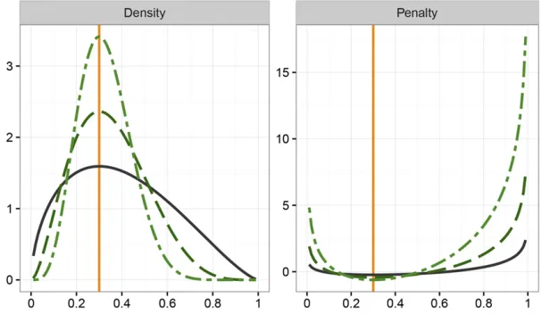
Figure 1 shows the probability density of a variable with a standard Beta distribution on the interval½0;1with mode of 0.3 together with the resulting penalty (i.e., minus the loga-rithmic value of the density), for three values of PSS. For

n. WhilePðuÞin (1) was considered nonnegative, penalty values close to the mode can be negative—this does not affect suitability of the penalty and can be overcome by add-ing a suitable constant.

Penalty on canonical eigenvalues: Canonical eigenvalues fall in the interval½0;1:Forqtraits, there are likely to beq

different valuesli and attempts to determine the mode of

their distribution may be futile. Hence we propose to sub-stitute the mean canonical eigenvalue,l:Taking minus log-arithmic values of (5) and assuming the same mode and PSS for allqeigenvalues then gives penalty

P_l¼C2ðn22Þ lX

q

i¼1

 logðliÞ þ

12l X

q

i¼1

 logð12liÞ

" #

(7)

with C¼qloghB1þlðn22Þ;1þ ð12lÞðn22Þi. This formulation results in shrinkage of all eigenvalues toward

l;with the highest and lowest values shrunk the most.

Penalty on correlations:Following Joe (2006) and Daniels and Pourahmadi (2009), we assume independent shifted Beta distributions on½21;1for PAC.

Daniels and Pourahmadi (2009) considered several Bayesian priors for correlation matrices formulated via PAC, suggesting uniform distributions for individual pij;

i.e.,pijBetað1;1Þ:In addition, they showed that the

equiv-alent to the joint uniform prior for R proposed by Barnard

et al. (2000),pðRÞ}1; is obtained by assuming Beta priors for PAC with shape parameters depending on the number of intervening variables;i.e.,ai;iþk¼bi;iþk¼1þ ðq212kÞ=2:

Similarly, priors proportional to higher powers of the de-terminant of R, pðRÞ}jRjt21; are obtained for ai;iþk¼

tþ ðq212kÞ=2 (Daniels and Pourahmadi 2009). Gaskins

et al. (2014) extended this framework to PAC-based priors with more aggressive shrinkage toward zero for higher lags, suitable to encourage sparsity in estimated correlation matri-ces for longitudinal data.

Both Joe (2006) and Daniels and Pourahmadi (2009) con-sidered Beta priors for PAC witha¼b;i.e., shrinkage of all

pijtoward zero. We generalize this by allowing for different

shrinkage targetstij—and thus different shape parametersaij

andbij—for individual valuespij:This gives penalty

Pp¼qðq₂21Þðn21Þlogð2Þ þX

q

i¼1

Xq

j¼iþ1

Cij

2n22

2

ðtijþ1Þlogðpijþ1Þ þ ð12tijÞlogð12pijÞ

(8)

with Cij¼log½Bð1þ ðtijþ1Þðn22Þ=2;1þ ð12tijÞðn22Þ=

2Þ:Again, this assumes equal PSS for all values, but could of course readily be expanded to allow for different valuesnijfor

different PACs. For alltij¼0;(8) reduces to

P_pð0Þ ¼ qðq21Þ

2

ðn21Þlogð2Þ þC0

2n22

2

Xq

i¼1

Xq

j¼iþ1

log

12p2ij

(9)

withC0 ¼log

Bð1þ ðn22Þ=2;1þ ðn22Þ=2Þ:

Maximizing the penalized likelihood

REML estimation in quantitative genetics usually relies on algorithms exploiting derivatives of the log-likelihood func-tion to locate its maximum. In particular, the so-called average information algorithm (Gilmour et al.1995) is widely used due to its relative computational ease, good convergence properties, and implementation in several REML software packages. It can be described as a Newton(–Raphson)-type algorithm where the Hessian matrix is approximated by the average of observed and expected information. To adapt the standard, unpenalized algorithm for penalized estimation we need to adjust first and second derivatives of logLðuÞ for derivatives of the penalties with respect to the parameters,

uk;to be estimated. These differ if we choosefixed values to

or the meanlifrom a preliminary, unpenalized analysis) or

employ penalties that derive these from the parameter estimates.

Canonical eigenvalues:Iflin (7) is estimated from the data, its derivatives are nonzero. This gives

@P_l

@uk

¼ @C

@uk

þ ðn22Þ @l

@uk Xq

i¼1

log 12li

li (

þX

q

i¼1

@li

@uk

12l 12li2

l li

!)

(10)

and

@2_P l

@uk@um

¼ @2C

@uk@um

þ ðn22ÞX

q

i¼1

@2_l

@uk@um

log 12li

li

2 @l @uk

@li

@um

þ@li

@uk

@l @um

1

li

þ 1

12li

þ @2li

@uk@um

12l 12li2

l li

þ@li

@uk

@li

@um

l l2

i

þ 12l

ð12liÞ2

: (11)

Derivatives of C involve the digamma and trigamma func-tions,e.g.,

@C @uk

¼qðn22Þ @l

@uk h

c1þ ðn22Þl

2c1þ ðn22Þð12lÞi

withcthe digamma function. Derivatives oflirequired in

(10) and (11) are easiest to evaluate if the analysis is pa-rameterized to the canonical eigenvalues and the elements of the corresponding transformation matrix T (see Meyer and Kirkpatrick 2010), so that@li=li¼1 and@l=li¼1=q

and all other derivatives of l and li are zero. A possible

approximation is to ignore contributions of derivatives of

l;arguing that the mean eigenvalue is expected to be un-affected by sampling overdispersion and thus should change little.

Partial correlations:Analogous arguments hold for penalties involving correlations. This gives

@P_p

@uk

¼X

q

i¼1

Xq

j¼iþ1

@Cij

@uk

þn22

2

"

log 12pij 1þpij

@tij

@uk

þ2 pij2tij

12p2_ij

@pij

@uk #

(12)

and

@2_P p

@uk@um

¼X

q

i¼1

Xq

j¼iþ1

@2_C

ij

@uk@um1

n22 2

"

log 12pij 1þpij

@2_t

ij

@uk@um

2 2

12p2

ij

@tij

@uk

@pij

@um1

@tij

@um

@pij

@uk

12 pij2tij 12p2_ij

@2_p

ij

@uk@um

22 12t

2

ijþ ðpij2tijÞ2

12p2

ij 2

!

@pij

@uk

@pij

@um #

(13)

with obvious simplifications if shrinkage targets arefixed or treated as such, so that derivatives oftijare zero. As shown in

theAppendix, derivatives of correlations and PACs are read-ily calculated from the derivatives of covariance compo-nents for any of the parameterizations commonly utilized in (unpenalized) REML algorithms for variance component estimation.

Simulation Study

A large-scale simulation study, considering a wide range of population parameters, was carried out to examine the effi -cacy of the penalties proposed above.

Setup

Data were sampled from multivariate normal distributions for

q¼9 traits, assuming a balanced paternal half-sib design composed ofsunrelated sire families with 10 progeny each. Sample sizes considered weres¼100;400, and 1000, with records for all traits for each of the progeny but no records for sires.

Population values for genetic and residual variance com-ponents were generated by combining 13 sets of heritabilities with six different types of correlation structures to generate 78 cases. Details are summarized in theAppendixand pop-ulation canonical eigenvalues for all sets are shown in Sup-plemental Material, File S1. To assess the potential for detrimental effects of penalized estimation, values were chosen deliberately to generate both cases that approxi-mately matched the priors assumed in deriving the penal-ties and cases where this was clearly not the case. The latter included scenarios where population canonical eigenvalues were widely spread and in multiple clusters and cases where genetic and phenotypic correlations were highly dis-similar. A total of 500 samples per case and sample size were obtained and analyzed.

Analyses

REML estimates ofSGandSEfor each sample were obtained

without penalization and imposing a penalty on canonical eigenvaluesP_l;as given in (7), and penalties on partial au-tocorrelations shrinking all values toward zero [Ppð0Þ;see

the latter, penalties on genetic PAC only and both genetic and residual values were examined.

Analyses were carried out consideringfixed values for the effective sample size, ranging fromn¼2:5 to 24. For penalties on both genetic and residual PAC, either the same value was used for both or the PSS for residual PAC wasfixed atn¼8:In addition, direct estimation of a suitable PSS for each replicate was attempted. As shown in (1), penalties were subtracted from the standard log-likelihood, incorporating a factor of 1=2: The model of analysis was a simple animal model, fitting means for each trait as the onlyfixed effects. A method-of-scoring algorithm together with simple derivative-free search steps was used to locate the maximum of the (penalized) likelihood func-tion. To facilitate easy computation of derivatives ofPl;this was

done using a parameterization to the elements of the canonical decomposition (see Meyer and Kirkpatrick 2010), restraining estimates oflito the interval of½0:0001;0:9999:

Direct estimation ofnwas performed by evaluating points on the profile likelihood forn[i.e., maximizing logLPðuÞwith

respect to the covariance components to be estimated for selected,fixed values ofn], combined with quadratic approx-imation steps of the profile to locate its maximum, using Powell’s (2006) Fortran subroutine NEWUOA. To avoid nu-merical problems, estimates ofnwere constrained to the in-terval ½2:01;50: All calculations were carried out using custom Fortran programs (available on request).

Summary statistics

For each sample and analysis, the quality of estimates was evaluated through their entropy loss (James and Stein 1961)

L1

SX;S^X

¼trS2X1S^X

2logS2X1S^X2q (14)

forX¼G;E, andP, withPXdenoting the matrix of

popula-tion values for genetic, residual, and phenotypic covariances andP^ _Xthe corresponding estimate. As suggested by Lin and Perlman (1985), the percentage reduction in average loss (PRIAL) was used as the criterion to summarize the effects of penalization

100

"

12L1

SX;S^

n

X .

L1

SX;S _0

X #

; (15)

where L1ðÞ denotes the entropy loss averaged over

repli-cates, and S^nX and S^

0

X represent the penalized and

corre-sponding unpenalized REML estimates ofSX;respectively.

In addition, the average reduction in logLðuÞ due to penalization, DL; was calculated as the mean difference across replicates between the unpenalized likelihood for

esti-matesS^nXand the corresponding value for estimatesS^

0

X: Data availability

The author states that all data necessary for confirming the conclusions presented in the article are represented fully within the article.

Results

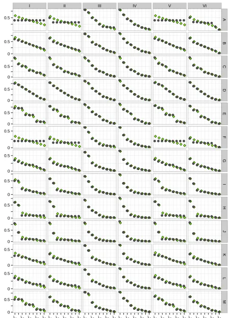
Distributions of PRIAL across the 78 sets of population values together with the corresponding change in likelihood are shown in Figure 2 for two sample sizes, with penalties

Ppð0ÞandPpðPÞapplied to genetic PAC only. Distributions

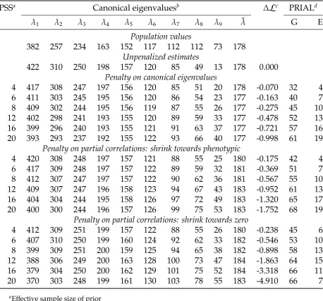
shown are trimmed; i.e., their range reflects minimum and maximum values observed. Selected mean and minimum val-ues are also reported in Table 1. More detailed results for individual cases are reported inFile S1.

Genetic covariances

Overall, forfixed PSS there were surprisingly few differences between penalties in mean PRIAL values achieved, especially for estimates of the genetic covariance matrix. Correlations between PRIAL for S^G from 0.9 to unity suggested similar

modes of action.

For comparison, additional analyses considered penalties on standard correlations, obtained by substitutingrijforpijin

(8), (9), (12), and (13). Corresponding PRIAL values (not shown) for these were consistently lower and, more impor-tantly, a considerable number of minimum values were neg-ative, even for small values of the PSS. Clearly this reflected a discrepancy between priors assumed and the distribution of correlations. Transformation to partial autocorrelation yield-ed a better match and thus yieldyield-ed penalties markyield-edly less likely to have detrimental effects. While easier to interpret than PAC, penalties on standard correlations based on inde-pendent Beta priors are thus not recommended.

Even for small values ofnthere were worthwhile reduc-tions in loss for estimates ofPG;in particular for the smallest

sample (s¼100). Means increased with increasing strin-gency of penalization along with an increasing spread in re-sults for individual cases, especially for the largest sample size. This pattern was due to the range of population values for genetic parameters used.

Moreover, for small samples or low PSS, it did not appear to be all that important whether the priors on which the penalties were based approximately matched population values or not:

“Any” penalty proved beneficial, i.e., resulted in positive PRIAL for S^G: For more stringent penalization, however,

there was little improvement (or even adverse effects) for the cases where there was a clear mismatch. For instance, forPlforn¼24 ands¼100 sires, there were two cases with

negative PRIAL forS^G:Both of these had a cluster of high

and low population values forliso that the assumption of

a unimodal distribution invoked in deriving Pl was

inap-propriate and led to sufficient overshrinkage to be detri-mental. On the whole, however, unfavorable effects of penalization were few and restricted to the most extreme cases considered.

Paradoxically, PRIAL values for P^G were also relatively

penalty function, as illustrated in Figure 1, resulting in little penalization for values close to the mode. In other words, these were cases were the prior also did not quite match the population values: While the assumption of a common mean for canonical eigenvalues clearly held, that of a distri-bution on the interval½0;1did not. This can be rectified by specifying a more appropriate interval. As the unpenalized estimates of li are expected to be overdispersed, their

ex-tremes may provide a suitable range to be used. Additional simulations (not shown) forPlreplaced values ofa¼0 and b¼1 used to derive Pl in (7) with a¼maxð0;^l920:05Þ

andb¼minð1;l^1þ0:05Þfor each replicate, where^l1 and

^

l9represented the largest and smallest canonical eigenvalue

estimate from a preliminary, unpenalized analysis, respec-tively. This increased PRIAL for bothP^G and ^

P

E

substan-tially for these cases. However, as the proportion of such cases was low (seeFile S1), overall results were little affected.

Residual covariances

Differences between penalties were apparent forSE:Pl

in-volved terms logð12liÞ[see (7)],i.e., the canonical

eigen-values ofSEandSP:Hence,Plyielded substantial PRIAL for

estimates of bothSGandSE;especially for the smaller

sam-ples where sampling variances and losses were high. Con-versely, applying penalties on genetic PAC resulted in some, but lower improvements inSE(except for largen), but only

as a by-product due to negative sampling correlations be-tweenSG and SE:As shown in Table 2, imposing a

corre-sponding penalty on residual PACs in addition could increase the PRIAL in estimates ofSEmarkedly without reduction in

the PRIAL forSG;provided the PSS chosen corresponded to a

relatively mild degree of penalization. Shrinking toward

phenotypic PAC yielded somewhat less spread in PRIAL for

SE than shrinking toward zero, accompanied by smaller

changes in logLðuÞ:

Phenotypic covariances

We argued above that imposing penalties based on the esti-mate ofSPwould allow us to borrow strength from it because

typicallySPis estimated more precisely than any of its

com-ponents. Doing so, we would hope to have little—and cer-tainly no detrimental—effect on the estimates ofSP:Loosely

speaking, we would expect penalized estimation to redress, to some extent at least, any distortion in partitioning of SP

due to sampling correlations. As demonstrated in Figure 2, this was generally the case forfixed values of the PSS less than n¼10 or 12. Conversely, negative PRIAL for esti-mates ofSP for higher values ofnflagged overpenalization

for cases where population values for genetic parameters did not sufficiently match the assumptions on which the penalties were based.

Canonical eigenvalues

Figure 3 shows the distribution of the largest and smallest canonical eigenvalues, contrasting population values with mean estimates from unpenalized and penalized analyses for a medium sample size and afixed PSS ofn¼8:Results clearly illustrate the upward bias in estimates of the largest and downward bias in estimates of the smallest eigenvalues. As expected, imposing penaltyPl reduced the mean of the

largest and increased the mean of the smallest eigenvalues, with some overshrinkage, especially of the largest eigen-value, evident. In contrast, for the small value ofn¼8 cho-sen, the distribution of the largest values from penalized and

Figure 2Distribution of percent-age reduction in averpercent-age loss for estimates of genetic, residual, and phenotypic covariance matrices, to-gether with corresponding change in log-likelihood (DL) for penalties on canonical eigenvalues (Pl) and

genetic, partial autocorrelations, shrinking toward zero [Ppð0Þ] or

phenotypic values [PpðPÞ].

unpenalized analyses differed little for penalty PpðPÞ; i.e.,

penalizing genetic PAC did not affect the leading canonical eigenvalues markedly, acting predominately on the smaller values. For more stringent penalties, however, some shrink-age of the leading eigenvalues due to penalties P_pðPÞ and

Ppð0Þ was evident; detailed results for selected cases are

given inFile S1.

Estimating PSS

On the whole, attempts to estimate the appropriate value ofn from the data were not all that successful. ForPl;numerous

cases yielded an estimate ofnclose to the lower end of the range allowed,i.e., virtually no penalty. Conversely, forPpð0Þ

andPpðPÞa substantial number of cases resulted in estimates

ofnclose to the upper bound allowed. This increased PRIAL (compared tofixed values forn) for cases that approximately matched the priors but caused reduced or negative PRIAL and substantial changes in logLðuÞotherwise. A possible ex-planation was that the penalized likelihood and thus the es-timate ofnmight be dominated byPE:However, as shown in

Table 2, neither estimating a value forSG(nG) whilefixing

the PSS forSE(nE) nor estimating a value for both (either

separately or jointly,nG¼nE) improved results greatly.

More-over, it yielded more cases for which penalization resulted in substantial, negative PRIAL, especially forPpðPÞ:Repeating

selected analyses using a sequential grid search to determine optimal values ofngave essentially the same results;i.e., re-sults could not be attributed to inadequacies in the quadratic approximation procedure. Given the additional computational requirements and the fact that suitable values could not be estimated reliably, joint estimation of PSS together with the covariance components cannot be recommended.

Discussion

Sampling variation is the bane of multivariate analyses in quantitative genetics. While nothing can replace large num-bers of observations with informative data and appropriate relationship structure, we often need to obtain reasonably trustworthy estimates of genetic parameters from relatively small data sets. This holds especially for data from natural populations but is also relevant for new or expensive to mea-sure traits in livestock improvement or plant breeding schemes. We have shown that regularized estimation in a maximum-likelihood framework through penalization of the likelihood function can provide“better”estimates of covari-ance components,i.e., estimates that are closer to the popu-lation values than those from standard, unpenalized analyses. This is achieved through penalties targeted at reducing sam-pling variation.

Table 1 Selected mean and minimum values for percentage reduction in average loss for estimates of genetic (SG), residual (SE), and

phenotypic (SP) covariance matrices together with mean change in unpenalized log-likelihood from the maximum (DL) for penalties on

canonical eigenvalues (Pl) and genetic correlations, shrinking partial autocorrelations toward zero [Ppð0Þ] or phenotypic values [PpðPÞ]

100 sires 400 sires 1000 sires

Penalty na _{SG SE SP DL SG SE SP DL SG SE SP DL}

Mean values

Pl 4 41 43 1 20.6 31 19 0 20.2 21 9 0 20.1

6 49 46 1 21.2 38 22 0 20.5 27 12 0 20.2

8 54 50 1 21.9 42 24 0 20.7 30 13 0 20.4

12 58 51 1 23.0 45 25 0 21.4 33 13 0 20.7

E 18 10 0 20.2 22 7 0 20.1 16 4 0 20.1

Ppð0Þ 4 47 13 1 20.9 37 5 0 20.3 27 2 0 20.2

6 53 21 1 21.8 43 9 0 20.7 31 4 0 20.4

8 56 26 2 22.9 44 12 0 21.1 32 6 0 20.6

12 58 31 2 25.1 45 16 1 22.1 34 8 0 21.1

E 56 29 3 28.5 46 12 1 21.9 35 5 0 20.5

PpðPÞ 4 46 9 0 20.7 37 3 0 20.3 26 1 0 20.2

6 52 15 0 21.4 42 6 0 20.7 31 2 0 20.4

8 55 21 0 22.0 44 8 0 21.0 32 3 0 20.6

12 57 28 1 23.1 45 11 0 21.6 33 5 0 21.0

E 60 47 2 28.7 50 22 1 23.5 36 10 0 21.7

Minimum values

Pl 8 12 26 0 22.9 5 7 0 21.7 2 2 0 21.1

12 1 13 0 24.7 211 11 21 23.0 214 4 21 22.2

E 0 4 0 20.7 1 1 0 20.6 1 0 0 20.4

P_pð0Þ 8 16 11 0 25.0 2 2 0 23.0 1 0 0 21.9

12 14 11 0 28.7 27 2 21 25.4 213 0 21 23.4

E 18 7 21 216.4 1 3 21 211.6 1 1 0 22.8

PpðPÞ 8 18 7 0 23.5 4 1 0 22.9 1 0 0 22.6

12 16 12 0 25.4 21 2 0 24.7 25 0 0 24.3

E 3 12 21 212.4 234 7 0 28.8 254 3 0 25.6

a_{Effective sample size of the Beta prior. Numerical values are“fixed”values used whileEdenotes values estimated from the data for each replicate, with means of 3.1, 5.9,}

Simplicity

The aim of this study was to obtain a procedure to improve REML estimates of covariance components and thus genetic parameters that is easy to use without considerable increase in computational requirements and suitable for routine aplica-tion. We have demonstrated that it is feasible to choose default values for the strength of penalization that yield worthwhile reductions in loss for a wide range of scenarios and are robust,

i.e., are unlikely to result in penalties with detrimental ef-fects, and are technically simple. While such a tuning-free approach may not yield a maximum reduction in loss, it ap-pears to achieve a substantial proportion thereof in most cases with modest changes in the likelihood compared to the maximum of logLðuÞ(without penalization). In contrast to earlier attempts to estimate a tuning factor (Meyer and Kirkpatrick 2010; Meyer 2011), it does not require multiple additional analyses to be carried out, and effects of penal-ization on computational requirements are thus mostly unimportant.

In addition, we can again make the link to Bayesian estimation, where the idea of mildly or weakly informative priors has been gaining popularity. Discussing priors for var-iance components in hierarchical models, Gelman (2006) advocated a half-t or half-Cauchy prior with large-scale

parameters. Huang and Wand (2013) extended this to prior distributions for covariance matrices that resulted in half-t priors for standard deviations and marginal densities of cor-relationsrproportional to a power ofð12r2_{Þ:Chunget al.}

(2015) proposed a prior for covariance matrices proportional to a Wishart distribution with a diagonal scale matrix and low degrees of belief to obtain a penalty on the likelihood function that ensured nondegenerate estimates of variance components.

Choice of penalty

We have presented two types of suitable penalties thatfit well within the standard framework of REML estimation. Both achieved overall comparable reductions in loss but acted slightly differently, with penalties on correlations mainly affecting the smallest eigenvalues of the covariance matrices while penalties on canonical eigenvalues acted on both the smallest and largest values. Clearly it is the effect on the smallest eigenvalues (which have the largest sampling vari-ances) that contributes most to the overall reduction in loss for a covariance matrix. An advantage of the penalty on correla-tions is that it is readily implemented for the parameteri-zations commonly employed in REML estimation, and it is straightforward to extend it to models with additional random effects and covariance matrices to be estimated or cases where

Table 2 Selected mean and minimum values for percentage reduction in average loss for estimates of genetic (SG), residual (SE), and

phenotypic (SP) covariance matrices together with mean change in unpenalized log-likelihood from the maximum (DL) for penalties on

both genetic and residual partial autocorrelations, shrinking toward zero [Ppð0Þ] or phenotypic values [PpðPÞ]

na _{100 sires 400 sires 1000 sires}

Penalty nG nE SG SE SP DL SG SE SP DL SG SE SP DL

Mean values

Ppð0Þ 4 4 48 38 1 20.9 37 16 0 20.4 27 7 0 20.2

8 4 56 43 2 22.9 45 20 0 21.1 33 10 0 20.6

8 8 57 48 2 22.8 45 23 1 21.1 33 12 0 20.6

E 4 57 46 3 26.6 48 21 1 21.3 35 10 0 20.5

E nG 61 55 3 25.3 50 27 1 21.8 37 14 0 20.8

E E 53 43 3 29.1 47 24 1 21.9 35 13 0 20.5

PpðPÞ 4 4 47 37 0 20.8 37 15 0 20.4 27 7 0 20.2

8 4 55 43 1 22.2 44 19 0 21.0 32 9 0 20.6

8 8 56 47 1 22.3 44 22 0 21.1 32 11 0 20.6

E 4 60 57 1 28.2 51 31 1 23.5 36 14 0 21.6

E nG 61 60 2 210.8 46 31 1 26.5 33 18 0 23.0

E E 61 60 2 210.7 51 33 1 24.9 36 15 0 22.3

Minimum values

Ppð0Þ 4 4 17 11 0 21.5 2 1 0 20.9 0 0 0 20.6

8 4 17 17 1 24.8 3 3 0 22.9 1 1 0 21.9

8 8 16 21 0 24.6 3 4 0 22.9 1 1 0 22.0

E 4 16 11 0 212.8 5 4 0 25.9 1 2 0 22.9

E nG 17 21 21 210.6 3 6 0 26.2 2 2 0 23.0

E E 270 2139 25 217.7 6 269 22 212.3 2 25 0 22.9

P_pðPÞ 4 4 20 10 0 21.3 2 1 0 21.0 0 0 0 20.8

8 4 21 20 0 23.7 4 3 0 23.0 1 1 0 22.7

8 8 20 23 0 23.8 5 5 0 23.1 1 1 0 22.7

E 4 5 24 21 210.8 228 9 0 27.9 248 3 0 24.9

E nG 23 10 21 217.0 232 228 23 216.0 265 1 21 28.5

E E 21 10 22 217.4 230 26 22 29.4 264 218 22 26.7

a_{Effective sample size of the Beta prior for genetic (nG) and residual (nE) correlations. Numbers given arefixed values used whileEdenotes values estimated from the data for}

traits are recorded on distinct subsets of individuals so that some residual covariances are zero. It also lends itself to scenarios where we may be less interested in a reduction in sampling variance but may want to shrink correlations toward selected target values.

Strength of penalization

Results suggest that penalties on canonical eigenvalues or PAC assuming a Beta prior with a conservative choice of PSS ofn¼4–10 will not only result in substantial improvements in estimates of genetic covariance components for many cases, but also result in little chance of detrimental effects for cases where the assumed prior does not quite match the underlying population values. Reanalyzing a collection of published heritability estimates from Mousseau and Roff (1987), M. Kirkpatrick (personal communication) sug-gested that their empirical distribution could be modeled as Betað1:14;1:32Þ; corresponding to v¼2:46 and mode of 0.3.

Additional bias

The price for a reduction in sampling variances from penalized analyses is an increase in bias. It is often forgotten that REML estimates of covariance components are biased even if no penalty is applied, as estimates are constrained to the param-eter space;i.e., the smallest eigenvalues are truncated at zero or, in practice, at a small positive value to ensure estimated matrices are positive definite. As shown in Figure 3, penali-zation tended to increase the lower limits for the smallest canonical eigenvalues and thus also for the corresponding values of the genetic covariance matrix, thus adding to the inherent bias. Previous work examined the bias due to penal-ization on specific genetic parameters in more detail (Meyer and Kirkpatrick 2010; Meyer 2011), showing that changes from unpenalized estimates were usually well within the range of standard errors. Employing a mild penalty withfixed PSS, changes in logLðuÞ from the maximum value in an unpenalized analysis were generally small and well below significance levels. This suggests that additional bias in REML estimates due to a mild penalty on the likelihood is of minor

concern and far outweighed by the benefits of a reduction in sampling variance.

Alternatives

Obviously, there are many other choices. As in Bayesian estimation, results of penalized estimation are governed by the prior distribution selected, the more so the smaller the data set available. Mean reductions in loss obtained in a previous study, attempting to estimate tuning factors and using pen-alties derived assuming a normal distribution of canonical eigenvalues or inverse Wishart distributions of covariance or correlation matrices, again were by and large of similar magnitude (Meyer 2011). Other opportunities to reduce sampling variation arise through more parsimonious model-ing, e.g., by estimatingSG at reduced rank or assuming a

factor-analytic structure. Future work should examine the scope for penalization in this context and consider the effects on model selection.

Application

Practical application of REML estimation using the simple penalties proposed is illustrated using the data set consid-ered by Meyer and Kirkpatrick (2010) (available as supple-mental material in their article). In brief, this was composed of six traits measured on beef cattle, with 912– 1796 records per trait. Including pedigree information on parents, grandparents, etc., without records yielded a total of 4901 animals in the analysis. The model of analy-sis fitted animals’ additive genetic effects as random and so-called contemporary group effects, with up to 282 levels per trait, asfixed. The latter was a subclass representing a combination of systematic environmental factors to ensure only animals subject to similar conditions were directly compared.

Estimates of SG and SE were obtained by REML using

WOMBAT (Meyer 2007), applying penalties on canonical ei-genvalues and partial correlations (shrinking toward zero) using PSS of 4 and 8, and contrasted to unpenalized results. Lower bound sampling errors for estimates of canonical

Figure 3 Distribution of mean estimates of selected ca-nonical eigenvalues comparing results from unpenalized analyses and analyses imposing penalties on canonical ei-genvalues (Pl) and genetic, partial autocorrelations,

shrinking toward phenotypic values [PpðPÞ], with

eigenvalues were approximated empirically (Meyer and Houle 2013).

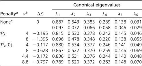
Results are summarized in Table 3. For all penalties and both levels of PSS, deviations in the unpenalized likelihood from the maximum (for the“standard”unpenalized analysis) were small and well below the significance threshold of–1.92 for a likelihood-ratio test involving a single parameter (at an error probability of 5%), emphasizing the mildness of penal-ization even for the larger PSS. Similarly, changes in esti-mates of canonical eigenvalues were well within their 95% confidence limits, except forl1forPlwithn¼8;which was

just outside the lower limit. As expected from simulation results above (cf. Figure 3), the penalty on canonical eigen-values affected estimates of the largest eigen-values more than penalties on partial correlations. Conversely, the latter yield-ed somewhat larger changes in the lowest eigenvalues. Esti-mates forPlwithn¼8 agreed well with results from Meyer

and Kirkpatrick (2010) (of 0.69, 0.50, 0.38, 0.27, 0.17, and 0.05 forl1–l6;respectively), which were obtained by

apply-ing a quadratic penalty on the canonical eigenvalues and using cross-validation to determine the stringency of penalization.

Corresponding changes in individual parameters were small throughout and again well within the range of95% confidence intervals (sampling errors derived from the in-verse of the average information matrix) for the unpenalized analysis. The largest changes in correlations occurred for the pairs of traits with the smallest numbers of records and the higher PSS. For instance, forPlthe residual correlation

be-tween traits 1 and 4 changed from 0.82 (with standard error of 0.17) to 0.65, whilePpð0Þon both genetic and residual

PAC reduced the estimate of the genetic correlation from 0.48 (standard error of 0.25) to 0.37. Plots with detailed results for individual parameters are given inFile S1.

In summary, none of the penalties applied changed esti-mates significantly and none of the changes in estimates of individual parameters due to penalization were questionable. Indeed, the larger changes described yielded values more in line with literature results for the traits concerned, suggesting that penalization stabilized somewhat erratic estimates based on small numbers of observations.

Implementation

Penalized estimation for the penalties proposed for fixed values ofnhas been implemented in our mixed-model pack-ageWOMBAT(available athttp://didgeridoo.une.edu.au/km/

wombat.php) (MEYER2007). ForP_la parameterization to the

elements of the canonical decomposition is used for ease of implementation, while penalties on correlations use the stan-dard parameterization to elements of the Cholesky factors of the covariance matrices to be estimated. Maximization of the likelihood is carried out using the average information algo-rithm, combined with derivative-free search steps where nec-essary to ensure convergence. Example runs for a simulated data set are shown inFile S1.

Experience with applications so far has identified small to moderate effects of penalization on computational require-ments compared with an unpenalized analysis, with the bulk of extra computations arising from derivative-free search steps used to check for convergence. The parameterization to the elements of the canonical decomposition, however, tended to increase the number of iterations required even without penalization. Detrimental effects on convergence behavior when parameterizing to eigenvalues of covariance matrices have been reported previously (Pinheiro and Bates 1996).

Convergence rates of iterative maximum-likelihood anal-yses are dictated by the shape of the likelihood function. Newton–Raphson-type algorithms, including the average in-formation algorithm, involve a quadratic approximation of the likelihood. When this is not the appropriate shape, the algorithm may become “stuck”and fail to locate the maxi-mum. This happens quite frequently for standard (unpenal-ized) multivariate analyses comprising more than a few traits when estimated covariance matrices have eigenvalues close to zero. For such cases, additional maximization steps using alternative schemes, such as expectation maximization-type algorithms or a derivative-free search, are usually beneficial. For small data sets, we expect the likelihood surface around the maximum to be relativelyflat. Adding additional“ infor-mation”through the assumed prior distribution (a.k.a. the penalty) can improve convergence by adding curvature to the surface and creating a more distinct maximum. Conversely, too stringent a penalty may alter the shape of the surface sufficiently so that a quadratic approximation may not be successful. Careful checking of convergence should be an in-tegral part of any multivariate analysis, penalized or not.

Conclusion

We propose a simple but effective modification of standard multivariate maximum-likelihood analyses to“improve” esti-mates of genetic parameters: Imposing a penalty on the

Table 3 Reduction in unpenalized likelihood (DL) for applied example together with estimates of canonical eigenvalues

Canonical eigenvalues Penaltya _nb _{DL l1 l2 l3 l4 l5 l6}

Nonec _{0 0.887 0.543 0.383 0.239 0.138 0.031} 0.097 0.072 0.066 0.058 0.046 0.029

Pl 4 20.195 0.815 0.530 0.378 0.242 0.145 0.046

8 21.395 0.696 0.478 0.348 0.220 0.138 0.055

P_pð0Þ 4 20.117 0.880 0.534 0.377 0.246 0.141 0.049 8 20.628 0.867 0.522 0.370 0.259 0.146 0.069 4,4 20.172 0.836 0.531 0.376 0.244 0.140 0.048 8,8 20.797 0.789 0.520 0.372 0.263 0.148 0.070

a_P

l;penalty on canonical eigenvalues; Ppð0Þ;penalty on partial correlations, shrinking toward zero with a single value denoting a penalty on genetic correla-tions only and two values denoting a penalty on both genetic and residual corre-lations.

b_{Effective sample size of the Beta prior.}

c_{Second line gives approximate sampling errors of estimates of canonical}

likelihood designed to reduce sampling variation will yield estimates that are on average closer to the population values than unpenalized values. There are numerous choices for such penalties. We demonstrate that those derived under the assumption of a Beta distribution for scale-free function of the covariance components to be estimated, namely gen-eralized heritabilities (a.k.a. canonical eigenvalues) and ge-netic correlations, are well suited and tend not to distort estimates of the total, phenotypic variance. In addition, in-voking a Beta distribution allows the stringency of penaliza-tion to be regulated by a single, intuitive parameter, known as effective sample size of the prior in a Bayesian context. Aim-ing at moderate rather than optimal improvements in esti-mates, suitable default values for this parameter can be identified that yield a mild penalty. This allows us to abandon the laborious quest to identify tuning factors suited to partic-ular analyses. Choosing the penalty to be sufficiently mild can all but eliminate the risk of detrimental effects and results in only minor changes in the likelihood, compared to unpenal-ized analyses. Mildly penalunpenal-ized estimation is recommended for multivariate analyses in quantitative genetics consider-ing more than a few traits to alleviate the inherent effects of sampling variation.

Acknowledgments

The Animal Genetics and Breeding Unit is a joint venture of the New South Wales Department of Primary Industries and the University of New England. This work was supported by Meat and Livestock Australia grant B.BFG.0050.

Literature Cited

Anderson, T. W., 1984 An Introduction to Multivariate Statistical Analysis, Ed. 2. John Wiley & Sons, New York.

Barnard, J., R. McCulloch, and X. Meng, 2000 Modeling covari-ance matrices in terms of standard deviations and correlations, with applications to shrinkage. Stat. Sin. 10: 1281–1312. Bickel, P. J., and E. Levina, 2008 Regularized estimation of large

covariance matrices. Ann. Stat. 36: 199_–227.

Bickel, P. J., and B. Li, 2006 Regularization in statistics. Test 15: 271–303.

Bouriga, M., and O. Féron, 2013 Estimation of covariance matri-ces based on hierarchical inverse-Wishart priors. J. Stat. Plan. Inference 143: 795_–808.

Cheverud, J. M., 1988 A comparison of genetic and phenotypic correlations. Evolution 42: 958–968.

Chung, Y., A. Gelman, S. Rabe-Hesketh, J. Liu, and V. Dorie, 2015 Weakly informative prior for point estimation of covari-ance matrices in hierarchical models. J. Educ. Behav. Stat. 40: 136–157.

Daniels, M. J., and R. E. Kass, 2001 Shrinkage estimators for co-variance matrices. Biometrics 57: 1173–1184.

Daniels, M. J., and M. Pourahmadi, 2009 Modeling covariance matrices via partial autocorrelations. J. Multivariate Anal. 100: 2352–2363.

Deng, X., and K.-W. Tsui, 2013 Penalized covariance matrix esti-mation using a matrix-logarithm transforesti-mation. J. Comput. Graph. Stat. 22: 494_–512.

Fisher, T. J., and X. Sun, 2011 Improved Stein-type shrinkage estimators for the high-dimensional multivariate normal covari-ance matrix. Comput. Stat. Data Anal. 55: 1909–1918. Gaskins, J. T., M. J. Daniels, and B. H. Marcus, 2014 Sparsity

inducing prior distributions for correlation matrices of longitu-dinal data. J. Comput. Graph. Stat. 23: 966–984.

Gelman, A., 2006 Prior distributions for variance parameters in hierarchical models. Bayesian Anal. 1: 515–533.

Gilmour, A. R., R. Thompson, and B. R. Cullis, 1995 Average in-formation REML, an efficient algorithm for variance parameter estimation in linear mixed models. Biometrics 51: 1440–1450. Green, P. J., 1987 Penalized likelihood for general semi-parametric

regression models. Int. Stat. Rev. 55: 245–259.

Hayes, J. F., and W. G. Hill, 1980 A reparameterisation of a ge-netic index to locate its sampling properties. Biometrics 36: 237_–248.

Hayes, J. F., and W. G. Hill, 1981 Modi_fications of estimates of parameters in the construction of genetic selection indices (_‘bending_’). Biometrics 37: 483_–493.

Hill, W. G., 2010 Understanding and using quantitative genetic variation. Philos. Trans. R. Soc. Lond. B Biol. Sci. 365: 73–85. Hsu, C. W., M. S. Sinay, and J. S. J. Hsu, 2012 Bayesian estimation

of a covariance matrix withflexible prior specification. Ann. Inst. Stat. Math. 64: 319–342.

Huang, A., and M. P. Wand, 2013 Simple marginally noninforma-tive prior distributions for covariance matrices. Bayesian Anal. 8: 439–452.

Huang, J. Z., N. Liu, M. Pourahmadi, and L. Liu, 2006 Covariance matrix selection and estimation via penalised normal likelihood. Biometrika 93: 85–98.

James, W., and C. Stein, 1961 Estimation with quadratic loss, pp. 361–379 inProceedings of the Fourth Berkeley Symposium on Mathematical Statistics and Probability, edited by J. Neiman. Uni-versity of California Press, Berkeley, CA.

Joe, H., 2006 Generating random correlation matrices based on partial correlations. J. Multivariate Anal. 97: 2177–2189. Johnson, N., S. Kotz, and N. Balakrishnan, 1995 Continuous

Uni-variate Distributions(Wiley Series in Probability and Mathemat-ical Statistics: Applied Probability and Statistics Section, Vol. 2, Ed. 2). John Wiley & Sons, New York.

Koots, K. R., J. P. Gibson, and J. W. Wilton, 1994 Analyses of published genetic parameter estimates for beef production traits. 2. Phenotypic and genetic correlations. Anim. Breed. Abstr. 62: 825_–853.

Lawley, D. N., 1956 Tests of signi_ficance for the latent roots of covariance and correlation matrices. Biometrika 43: 128–136. Ledoit, O., and M. Wolf, 2004 A well-conditioned estimator for

large-dimensional covariance matrices. J. Multivariate Anal. 88: 365–411.

Ledoit, O., and M. Wolf, 2012 Nonlinear shrinkage estimation of large-dimensional covariance matrices. Ann. Stat. 40: 1024– 1060.

Lin, S. P., and M. D. Perlman, 1985 A Monte Carlo comparison of four estimators of a covariance matrix, pp. 411–428 in Multivar-iate Analysis, Vol. 6, edited by P. R. Krishnaish. North-Holland, Amsterdam.

Meyer, K., 2007 WOMBAT– a tool for mixed model analyses in quantitative genetics by REML. J. Zhejiang Univ. Sci. B 8: 815–821. Meyer, K., 2011 Performance of penalized maximum likelihood in estimation of genetic covariances matrices. Genet. Sel. Evol. 43: 39.

Meyer, K., and D. Houle, 2013 Sampling based approximation of confidence intervals for functions of genetic covariance matri-ces. Proc. Assoc. Adv. Anim. Breed. Genet. 20: 523–526. Meyer, K., and M. Kirkpatrick, 2010 Better estimates of genetic

Meyer, K., and S. P. Smith, 1996 Restricted maximum likelihood estimation for animal models using derivatives of the likelihood. Genet. Sel. Evol. 28: 23–49.

Meyer, K., M. Kirkpatrick, and D. Gianola, 2011 Penalized maxi-mum likelihood estimates of genetic covariance matrices with shrinkage towards phenotypic dispersion. Proc. Assoc. Adv. Anim. Breed. Genet. 19: 87–90.

Morita, S., P. F. Thall, and P. Müller, 2008 Determining the effec-tive sample size of a parametric prior. Biometrics 64: 595–602. Mousseau, T. A., and D. A. Roff, 1987 Natural selection and the

heritability of_fitness components. Heredity 59: 181_–197. Pinheiro, J. C., and D. M. Bates, 1996 Unconstrained

parameter-izations for variance-covariance matrices. Stat. Comput. 6: 289_–296.

Pourahmadi, M., 2013 High-Dimensional Covariance Estimation (Wiley Series in Probability and Statistics). John Wiley & Sons, New York/Hoboken, NJ.

Powell, M., 2006 The NEWUOA software for unconstrained opti-mization without derivatives, pp. 255–297 inLarge-Scale Nonlin-ear Optimization(Nonconvex Optimization and Its Applications, Vol. 83), edited by G. Pillo and M. Roma. Springer, US. Rapisarda, F., D. Brigo, and F. Mercurio, 2007 Parameterizing

cor-relations: a geometric interpretation. IMA J. Manag. Math. 18: 55. Roff, D. A., 1995 The estimation of genetic correlations from phe-notypic correlations - a test of Cheveruds conjecture. Heredity 74: 481–490.

Rothman, A. J., E. Levina, and J. Zhu, 2010 A new approach to Cholesky-based covariance regularization in high dimensions. Biometrika 97: 539–550.

Schäfer, J., and K. Strimmer, 2005 A shrinkage approach to large-scale covariance matrix estimation and implications for func-tional genomics. Stat. Appl. Genet. Mol. Biol. 4: 32.

Stein, C., 1975 Estimation of a covariance matrix, inReitz Lecture of the 39th Annual Meeting of the Institute of Mathematical Statistics. Atlanta, Georgia.

Thompson, R., S. Brotherstone, and I. M. S. White, 2005 Estimation of quantitative genetic parameters. Philos. Trans. R. Soc. Lond. B Biol. Sci. 360: 1469–1477.

Waitt, D. E., and D. A. Levin, 1998 Genetic and phenotypic cor-relations in plants: a botanical test of Cheverud’s conjecture. Heredity 80: 310–319.

Warton, D. I., 2008 Penalized normal likelihood and ridge regu-larization of correlation and covariance matrices. J. Am. Stat. Assoc. 103: 340–349.

Witten, D. M., and R. Tibshirani, 2009 Covariance-regularized regression and classification for high dimensional problems. J. R. Stat. Soc. B 71: 615–636.

Won, J.-H., J. Lim, S.-J. Kim, and B. Rajaratnam, 2013 Condition-number-regularized covariance estimation. J. R. Stat. Soc. B 75: 427–450.

Ye, R. D., and S. G. Wang, 2009 Improved estimation of the co-variance matrix under Stein’s loss. Stat. Probab. Lett. 79: 715–721.

Zhang, X., W. J. Boscardin, and T. R. Belin, 2006 Sampling cor-relation matrices in Bayesian models with correlated latent var-iables. J. Comput. Graph. Stat. 15: 880–896.

Appendix

Population Values

Population values for the 13 sets of heritabilities used are summarized in Table A1. The six constellations of genetic (rG ij) and

residual (rE ij) correlations between traitsiandj(i6¼j) were obtained as

I. rG ij ¼rE ij¼0;

II. rG ij¼0:5 andrE ij¼0:3;

III. rG ij¼0:7

ji2jj_andr

E ij ¼0:5þ0:05i ð21Þ j_;

IV. rG ij¼ 20:7

ji2jj_þ0:02iandr

E ij¼0:5þ ð20:2Þ

ji2jj_;

V. rG ij¼rE ij¼0:7 fori;j2 ½3;7andrG ij ¼rE ij¼0:3 otherwise, and

VI. rG ij¼rE ij¼0:6 forji2jj ¼1;andrG ij ¼rE ijcomputed from (4) withpij¼0:4 otherwise.

Phenotypic variances were equal to 1 throughout for correlation I and set to 2, 1, 3, 2, 1, 2, 3, 1, and 2 for traits 1–9 otherwise.

Derivatives of Partial Autocorrelations

Partial autocorrelations [see (3)] can be written as

pij¼cij= ffiffiffiffiffiffiffiffiffiv1v3

p

with

cij¼rij2r91R221r3

vx¼12r9xR221rx for x¼1;3:

This gives partial derivatives ofpijwith respect to parametersukandum:

@pij

@uk

¼@cij

@uk

pij

cij2

pij

2 1

v1

@v1

@uk

þ 1

v3

@v3

@uk

@2_p

ij

@uk@um

¼ ffiffiffiffiffiffiffiffiffi1

v1v3

p "

@2_c

ij

@uk@um2

1 2

@cij

@uk

1

v1

@v1

@um

þ1

v3

@v3

@um #

þpij

2 1

v12

@v1

@uk

@v1

@um2

1

v1

@2_v 1

@uk@um

þ 1

v32

@v3

@uk

@v3

@um2

1

v3

@2_v 3

@uk@um

21

2

@pij

@um

1

v1

@v1

@uk

þ 1

v3

@v3

@uk

:

Derivatives of the components are

@cij

@uk

¼@rij

@uk

þr91R221

@R2

@ukR 21

2 r32r91R221

@r3

@uk2

@r91

@ukR 21 2 r3 

@2_c

ij

@uk@um

¼ @2rij

@uk@um2

@2_r9 1

@uk@umR 21

2 r32r91R221

@2_r 3

@uk@um

þr91R221

@2_R 2

@uk@umR 21 2 r32@r91

@uk

R21 2

@r3

@um2

@r91

@umR 21 2

@r3

@uk

þ@r91

@ukR 21 2

@R2

@umR 21

2 r3þr91R221

@R2

@umR 21 2

@r3

@uk

þ@r91

@umR 21 2

@R2

@ukR 21

2 r3þr91R221

@R2

@ukR 21 2

@r3

@um

2r91R221

@R2

@umR 21 2

@R2

@ukR 21

2 r32r91R221

@R2

@ukR 21 2

@R2

@umR 21 2 r3

and

@vx

@uk

¼r9xR221

@R2

@ukR 21

2 rx22 r9xR221

@rx

@2_v

x

@uk@um¼r9xR 21 2

@2_R 2

@uk@umR 21

2 rx22  @

2_r9

x

@uk@umR 21 2 rx

þ2  @r9x

@umR 21 2

@R2

@uk

R21 2 rx

22 r9xR221

@R2

@umR 21 2

@R2

@uk

R21 2 rx

22  @r9x

@uk

R21 2

@rx

@um

þ2  @r9x

@uk

R21 2

@R2

@umR 21 2 rx:

Decompose the correlation matrix as R¼S21SS21 with S¼Diagfsig the diagonal matrix of standard deviations for

covariance matrixS:This gives the required derivatives of the correlation matrix:

@R @uk

¼S21@S

@ukS

21_2S21@S

@ukR2R

@S @ukS

21

@2_R

@uk@um

¼S21 @2S

@uk@umS

21_2S21 @2S

@uk@umR2R

@2_S

@uk@umS 21

2 S21@S

@umS 21@S

@ukS

21_2S21@S

@ukS

21@S

@umS 21

þ R@S

@ukS

21@S

@umS

21_þS21@S

@umS 21@S

@ukR

2 S21@S

@uk

@R @um2

@R @um

@S @ukS

21_:

Finally, assuming derivatives of variancessiiare available, the required derivatives of standard deviationssi¼pffiffiffiffiffiffisiiare

@si

@uk

¼ 1

2si

@sii

@uk

@2_s

i

@uk@um

¼ 1

2si

@2_s

ii

@uk@um2

1 2s2

i

@sii

@uk

@sii

@um

:

When estimating elements ofSdirectly, only@sii=@sii¼1 are nonzero. Derivatives of covariance matrices when employing a

parameterization to the elements of their Cholesky factors are given by Meyer and Smith (1996).

Table A1 Population values (3100) for sets of heritabilities

Trait no.

Set 1 2 3 4 5 6 7 8 9

A 40 40 40 40 40 40 40 40 40

B 60 55 50 45 40 35 30 25 20

C 90 60 50 50 30 30 20 20 10

D 75 70 60 50 40 30 20 10 5

E 70 70 70 40 40 40 10 10 10

F 20 20 20 20 20 20 20 20 20

G 35 30 25 20 20 20 15 10 5

H 60 50 10 10 10 10 10 10 10

I 50 50 20 15 15 10 10 5 5

J 80 40 10 10 10 10 10 5 5

K 30 30 25 25 20 15 15 10 10

L 35 30 30 20 20 15 15 15 10

GENETICS

Supporting Information

www.genetics.org/lookup/suppl/doi:10.1534/genetics.115.186114/-/DC1

Simple Penalties on Maximum-Likelihood Estimates

of Genetic Parameters to Reduce Sampling Variation

Karin Meyer