ABSTRACT
NABAVI, SEYEDBEHZAD. Measurement-Based Methods for Model Reduction, Identification, and Distributed Optimization of Power Systems. (Under the direction of Aranya Chakrabortty.)
In this dissertation, we develop algorithms for identification and distributed oscillation monitoring of large scale power system networks. In Part I, we propose two algorithms to identify reduced-order inter-area models of large power systems using the measurements of voltages and currents available from Phasor Measurement Units (PMUs) at some designated buses. In Chapter 2, we propose an algorithm that uses PMU measurements to identify the linear equivalent power system model. For this, we first extract the slow oscillatory components of the available PMU measurements using either state estimation or modal decomposition, and use the extracted components to construct the linear state-space model of the reduced-order system using nonlinear least squares. We validate our results using a detailed study of NPCC 48-machine system. In Chapter 3, we propose an algorithm to identify the nonlinear DAE model of the reduced-order power systems.
In Chapter 4, we investigate the identifiability of linear network dynamic systems exhibiting continuous-time weighted consensus defined over a class of graphs. Following the classical definition of output distinguishability, we first derive conditions that ensure the identifiability of the edge weights of the network graph in terms of its Markov parameters, and thereafter propose a sensor placement algorithm that guarantees a one-to-one mapping from the weights to these Markov parameters obtained from the available state measurements.
© Copyright 2015 by Seyedbehzad Nabavi
Measurement-Based Methods for Model Reduction, Identification, and Distributed Optimization of Power Systems
by
Seyedbehzad Nabavi
A dissertation submitted to the Graduate Faculty of North Carolina State University
in partial fulfillment of the requirements for the Degree of
Doctor of Philosophy
Electrical Engineering
Raleigh, North Carolina 2015
APPROVED BY:
Mo-Yuen Chow Edgar Lobaton
Ralph Smith Aranya Chakrabortty
DEDICATION
To my beloved family
My parents: Fereshteh Rajabzadeh, and Sirous Nabavi My siblings: Behrouz, Beheshteh, Behnam, and Banafsheh
BIOGRAPHY
Behzad Nabavi was born in Bojnord, North Khorasan, Iran in 1986. He received the B.S. degree from Amirkabir University of Technology (Tehran Polytechnic), Tehran, Iran, in 2009, and the M.S. degree from North Carolina State University, Raleigh, NC, USA, in 2011.
ACKNOWLEDGEMENTS
First and foremost, I would like to express my sincere gratitude to my advisor, Dr. Aranya Chakrabortty who gave me this great opportunity to be a part of his research group. His energy, guidance, support, and advice were a valuable assist not only to develop this work, but also to grow my personality during these four years. I would also like to thank Dr. Mo-Yuen Chow, Dr. Edgar Lobaton, and Dr. Ralph Smith for being part of my graduate committee and for letting me learn from their experience in the field.
I express my gratitude to Dr. Pramod Khargonekar of University of Florida for all his precious help and comments about the identifiability problem, as well as Dr. Rakesh Bobba, and Dr. Nitin Vaidya, for their constructive comments on the resiliency of distributed algorithms.
I am thankful for all the amazing educators I have worked alongside. I am also thankful to the family of FREEDM Systems Center for providing the friendly atmosphere for us to grow in and learn. I would like to appreciate all my labmates for their collaboration, help, guidance, hint, and feedback: Saman Babaei, Babak Parkhideh, Thomas R. Nudell, Vahraz Zamani, Nima Yoosefpour, Almuataz Boker, Hesam Mirzaei, Mohammad Etemadrezaei, Ghazal Falahi, Pouria Fajri, Sina Parhizi, Mahsa Kashani, Alireza Afiat, Maziar Mobarrez, Abhishak Jain, Jianhua Zhang, Urvir Singh, Mohammad Ali Rezaei, Yashar Naeimi, Bharadwaj Vasudevan, Govind Chavan, Kathleen Sico, Sarah Hambridge, and many others.
TABLE OF CONTENTS
LIST OF TABLES . . . vii
LIST OF FIGURES . . . .viii
Chapter 1 Introduction . . . 1
I Identification of Reduced-Order Models of Power Systems 3 Chapter 2 Identification of Equivalent Linear Dynamic Models of Power Sys-tems . . . 4
2.1 Introduction . . . 4
2.2 Problem Formulation . . . 7
2.2.1 Electromechanical Model of Power System . . . 7
2.2.2 Model Reduction of Power System Based on Slow Coherency . . . 9
2.2.3 The Model-Based Reduction of Large Power Systems . . . 11
2.3 The Proposed Identification Method . . . 12
2.3.1 Step 1. Construction of ∆δsk(t) fromy(t) . . . 13
2.3.2 Step 2. Estimation ofAs . . . 14
2.4 Case Studies . . . 15
2.4.1 Identification using state estimation . . . 16
2.4.2 Identification using modal decomposition . . . 18
2.4.3 Validating the results . . . 20
2.5 Conclusions . . . 22
Chapter 3 Identification of DAE Equivalent Models of Power Systems. . . 24
3.1 Problem Formulation . . . 26
3.1.1 Comparison with Chapter 2 . . . 29
3.2 The Proposed Structured-Identification Approach . . . 30
3.3 Case Study 1 . . . 36
3.3.1 Estimation ofx0ds k . . . 36
3.3.2 Estimation of inter-area parameters . . . 36
3.3.3 Identification of inter-area impedances . . . 37
3.4 Case Study 2 . . . 39
3.4.1 Calculating ˆVpsk(t)∠θˆspk(t) and ˆIpsk(t)∠φˆspk(t) for Area k . . . 40
3.4.2 Estimation ofx0ds k and r s k . . . 42
3.4.3 Estimating the remaining area parametersMks,Dks,Pmsk . . . 42
3.4.4 Identification of the inter-area impedances . . . 43
3.5 Conclusions . . . 44
Chapter 4 Identifiability Analysis of Weighted Consensus Networks . . . 45
4.2 Preliminaries . . . 47
4.3 Problem Formulation . . . 48
4.4 The Proposed Sensor Placement Algorithm . . . 49
4.4.1 Main Result . . . 49
4.4.2 Number of sensors needed . . . 56
4.4.3 Example . . . 57
4.4.4 More Information on Weights from a Transfer Function . . . 57
4.5 Examples . . . 58
4.5.1 Illustrating the one-to-one mapping between weights and the Markov parameters . . . 58
4.5.2 Sufficiency vs Necessity . . . 59
4.6 A Note on Star Graphs . . . 60
4.7 Extension to a Class of Cyclic Graphs . . . 62
4.7.1 Preliminary Assumptions . . . 62
4.7.2 The Sensor Placement Algorithm . . . 63
4.8 Conclusions . . . 72
II Distributed Algorithms for Power System Monitoring 73 Chapter 5 Distributed Estimation of Oscillation Modes. . . 74
5.1 Introduction . . . 74
5.2 Problem Formulation . . . 77
5.3 Modal Estimation using Prony Method . . . 78
5.4 Proposed Strategies for Distributed Modal Estimation . . . 80
5.4.1 Architecture 1: Distributed Prony using Standard ADMM (S-ADMM) . . 81
5.4.2 Architecture 1 with Asynchronous Communication . . . 84
5.4.3 Architecture 2: Distributed Prony using Distributed ADMM (D-ADMM) 86 5.4.4 Architecture 3–Distributed Prony using Hierarchical ADMM (H-ADMM) 89 5.5 Case Studies . . . 91
5.5.1 IEEE 68-bus Model . . . 91
5.5.2 IEEE 145-bus Model . . . 96
5.6 Real-Time Simulations using ExoGENI . . . 97
5.7 Conclusions . . . 99
Chapter 6 An Intrusion Resilient Distributed Modal Estimation . . . .100
6.1 Introduction . . . 100
6.2 Distributed Prony using D-ADMM . . . 101
6.3 A Case Study . . . 104
6.4 Conclusions . . . 108
Chapter 7 Conclusions and Future Works . . . .110
LIST OF TABLES
Table 2.1 PMUs placed per area . . . 19 Table 2.2 Post-fault oscillatory modes of the ∆ˆδs
i(t) for the NPCC 48-machine in the frequency range [0.1, 1] Hz obtained from Prony . . . 20 Table 2.3 The calculated values of the error termJa(k) as defined in (2.16) using the
model-based reduction, Case 1, and Case 2. Note that the trajectory of area 7 is the reference angle and it is zero by assumption. . . 22 Table 2.4 The inter-area modes of the reduced-order systems compared with the
full-order model . . . 23 Table 3.1 Estimation results of the generator parameters for the WECC model . . . 37 Table 3.2 Results of modal analysis ofVp ,[Vp1 Vp2 Vp3 Vp4]
T andθ
p ,[θp1 θp2 θp3 θp4]
T using Prony. The listed eigenvalues are those with frequencies in the range of [0.1, 1] Hz . . . 41 Table 3.3 Estimation results of the equivalent generator parameters for the IEEE 39-bus
model . . . 42 Table 4.1 Examples of sensor placement based on Algorithm 1 with N number of
sensors. The listed Markov parameters show their one-to-one relationship with the unknown edge-weights. . . 59 Table 5.1 Comparison between three different architectures . . . 91 Table 5.2 The estimated slow eigenvalues of the IEEE 68-bus model using centralized
Prony (Steps 1 and 2), and the distributed Prony algorithms atk= 50 . . . 94 Table 5.3 The computational area partitioning of the IEEE 145 bus model. The buses
written in boldface are equipped with PMUs (10 PMUs per area) . . . 96 Table 5.4 T1: measurement exchange streaming delay, T2: computation delay,T3:
aver-aging plus parameter exchanging delay (All time delays are measured for a single iteration, units are in milliseconds). . . 99 Table 6.1 The estimated slow eigenvalues of the IEEE 68-bus model in the two scenarios
LIST OF FIGURES
Figure 2.1 The discrepency between the actual measurement from the prediction of the
models, taken from [12] . . . 6
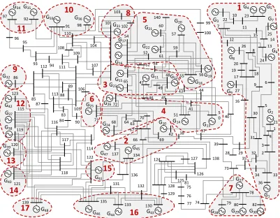
Figure 2.2 The one-line diagram of NPCC 48 machine system . . . 16
Figure 2.3 PCA-based generator clustering results using their rotor angles . . . 17
Figure 2.4 NPCC 48-machine model post-fault generator angles per area . . . 18
Figure 2.5 The topology of the identified reduced-order system in Case 1 . . . 19
Figure 2.6 Time response of 3 equivalent machines, black: actual response, red: the model-based reduced order model, blue: the identified model in Case 1 . . . 21
Figure 3.1 The reduction taking place in Chapter 3 . . . 28
Figure 3.2 Merging the boundary buses and forming a single equivalent pilot bus . . . 31
Figure 3.3 The equivalent model of a coherent area . . . 34
Figure 3.4 9-Bus WECC Model . . . 35
Figure 3.5 The relative error of the results in (3.18) calculated using (3.19) . . . 38
Figure 3.6 IEEE 39-bus model divided into four coherent areas. . . 38
Figure 3.7 The trajectories of Vi and θi at the buses with PMUs in IEEE 39-bus model. 39 Figure 3.8 The actual and the slow components of the equivalent pilot buses for the IEEE 39-bus model obtained in Step 1. . . 40
Figure 3.9 The matching between the obtained ∆ˆδs(t) and ∆δCOI(t) calculated using measurements as defined in (3.20) . . . 41
Figure 3.10 The matching between the ωs of the DAE model (3.14) and the ˆωs obtained in Step 3.1 from measurements . . . 41
Figure 3.11 The relative error of the results shown in (3.21) calculated using (3.19). . . 43
Figure 3.12 The equivalent DAE model of the IEEE 39-bus model. . . 44
Figure 4.1 Two networks with the same input-output transfer function as shown in (4.1) 46 Figure 4.2 The subgraph Hdefined in Lemma 4.4.2 . . . 52
Figure 4.3 Application of Algorithm 1 to T1 (circles indicate sensor nodes) . . . 53
Figure 4.4 S0∪S1 . . . 54
Figure 4.5 The set of children of nodeq0 ∈Sk . . . 55
Figure 4.6 The star graph of Proposition 4.6.1 . . . 61
Figure 4.7 Examples of graphs satisfying (4.20). The input is applied to node 1. . . 63
Figure 4.8 A network graph not satisfying Assumption 2. . . 64
Figure 4.9 Application of Algorithm 2 to a given graph G (circles indicate sensor nodes) 66 Figure 4.10 S0,S1, and a portion of S2 . . . 68
Figure 4.11 A subgraph of G discussed in Steps 2.1-2.5 . . . 70
Figure 5.1 Distributed architecture for wide-area PMU-PDC communications . . . 76
Figure 5.2 Architecture 1 using S-ADMM for a 4-area network. . . 81
Figure 5.3 Architecture 2 using D-ADMM for a given communication graph G for a 4-area network. . . 86
Figure 5.5 IEEE 68-bus model. . . 91 Figure 5.6 The estimation of σ and Ω per iterationk (solid lines) versus their actual
values obtained from PST (dashed lines). (a) S-ADMM algorithm. (The values are calculated at the ISO from ¯ak based on the Step 2 of the Prony algorithm.) (b) A-ADMM. (c) D-ADMM withG1. (The values are calculated using ak1.) (e) H-ADMM. . . 93 Figure 5.7 The communication graphs used in Architecture 2. . . 94 Figure 5.8 Comparison of the error term E(k) = P5
j=112kHˆja
k
j −ˆcjk22 for the four
proposed algorithms per iteration. . . 95 Figure 5.9 The estimation of σ and Ω using S-ADMM for the 145-bus model . . . 97 Figure 5.10 The execution flowchart of the distributed Prony using S-ADMM . . . 98 Figure 6.1 The D-ADMM architecture suitable for attack localization applied to a
4-area network. . . 102 Figure 6.2 IEEE 68-bus model. . . 105 Figure 6.3 (a) The communication graph used in Scenario 1 and Scenario 2 (only before
detection of the attack at PDC 3). (b) The reconfigured communication graph after detection of the attack at PDC 3 at scenario 3. . . 105 Figure 6.4 Scenario 1: (a) Error per PDC per iteration, (b) Estimation of a selected
set of σ’s per iteration at PDC 1, (c) Estimation of a selected set of Ω’s per iteration at PDC 1 . . . 106 Figure 6.5 Scenario 2: the calculated errors at each PDC described in D-ADMM
Chapter 1
Introduction
The power systems are the largest and the most complex man-made networks, comprised of millions of components. The grid conditions are changing continuously due to instantaneous changes in demand and hence the necessary changes in electricity generations. One of the challenges of the power system since its beginning has been to ensure its stability under such dynamically changing conditions at all times. Recently, due to the increase in the electricity demand, advent of highly penetrated renewable energy resources, as well as the electric vehicles, the network is pushed more toward its limits, and, therefore, the reliable performance of the grid will not be attainable without its real-time monitoring and control.
The advent of the GPS-synchronized measurement devices known as Phasor Measurement Units (PMUs) in recent years has enabled the operators and utilities to visualize and measure the network quantities with a very high sampling-rate (30 to 60 samples per second) and a high precision compared to the conventional technologies [1]. This very high volume of data generated by PMUs can be used in Wide-Area Measurement Systems (WAMSs) in order to ensure the reliability, stability, and security of the grid, both in real-time applications and the offline studies such as power systems planning and post-fault analyses.
grids. This dissertation is prepared in two parts. Part 1 mostly discusses the identification of the reduced-order power systems using the PMU measurements. The reduced-order power systems can be useful tools to study the dynamics of power systems in large-scales, building stability metrics, localization of disturbance, and designing the controllers, to name a few. Chapters 2 and 3 proposes methods to identify such models. Chapter 4 presents the preliminary results on the problem of sensor selection for general network dynamic systems with acyclic structures. These results can be generalized to the case of power system networks.
Part I
Identification of Reduced-Order
Chapter 2
Identification of Equivalent Linear
Dynamic Models of Power Systems
2.1
Introduction
Recent analyses of phase angle and frequency oscillations in the Western Electricity Coordinat-ing Council (WECC) and the Eastern Interconnect (EI) have highlighted the importance of constructing dynamic models of large power systems from Synchrophasor measurements [1, 2]. However, given the large size of any realistic power system, such as the WECC or EI, it is practically impossible to derive the pre-event or post-event dynamic model for the entire network in real-time. System operators are, rather, more interested in constructing reduced order models of the power system that capture the dominant inter-area modes of oscillation, and, hence, can predict how the different parts of the system may oscillate with respect to each other in the face of a particular contingency. Such reduced-order models are often referred to as wide-area
Mathematical modeling of dynamic equivalents of large-scale electric power systems has seen some 40 years of long and rich research history. The foundations of this research lineage were laid in the late 70s by Chow and Kokotovic who established the relationship between the slow coherency and weak connections in power systems using singular perturbation theory. They proposed algorithms of partitioning a power network into dynamic aggregates orcoherentareas, where each coherent area consists of a group of strongly connected generators that oscillates with fast time-scale against each other. The areas themselves are oscillating against each other with slower inter-area oscillatory modes across weakly connected power transfer interfaces. Their approach was complimented by alternative techniques of coherency [5], circuit-theoretic approaches [6], linear modal decomposition [7], and enumerative clustering algorithms [8]. Aggregation and coherency also was tested offline on both small-scale (such as 48-machine NPCC) and large-scale (such as 12000 bus NYPP2) via software programs such as DYNEQ and DYNRED [9].
However, the discrepancy between the offline models and the real-time events sometimes has caused severe catastrophic blackouts and cascaded failures. For example, Fig. 2.1 illustrates the mismatch between the recorded behavior of the WECC model during the blackout of August 10, 1996 versus the predicted results from the comprehensive simulation models. This figure clearly emphasizes the crucial need to build more accurate predictive models for long-range planning studies, short-range planning studies, near-term operations planning studies, and real-time on-line studies.
However, broadly speaking, the main limitations of the above-mentioned conventional model reduction methods are as follows:
–First, they are model-based methods, meaning that to construct reduced order models using these methods one would need to know each constituent model explicitly.
–Third, any model-based method provides a reduced-order approximation of the original system. While these approximated models provide a very accurate reduced-order representations of ideally-clustered systems, their accuracy declined for non-ideally clustered, realistic power system networks.
Figure 2.1: The discrepency between the actual measurement from the prediction of the models, taken from [12]
In Chapter 2 we proposed a measurement-based approach to obtain these reduced-order models.
the areas are not known apriori. The identified linear reduced-order models are directly in Krons form and do not retain any PV or PQ buses of the full-order model. These models are highly useful if operators want to evaluate the effective coupling strength between different coherent areas during a disturbance event. They can also be highly useful for assessing transient stability of inter-area dynamics of multi-area power systems by using energy functions, as shown in [22], where potential energy functions were estimated using the inter-area topology.
A preliminary version of this work was recently presented in [21]. The results in this chapter are, in comparison, significantly more advanced. In [21], we assumed the availability of generator state measurements for identification, while in this chapter we propose two algorithms to construct the states of the reduced-order model. The case studies presented here are much more detailed than those in [21] with their in-depth validation.
The remainder of Chapter 2 is organized as follows: Section 2.2 presents the power system models of interest. Section 2.3 proposes the topology identification method. Section 2.4 illustrates the results through several case studies. Section 2.5 concludes the chapter.
2.2
Problem Formulation
2.2.1 Electromechanical Model of Power System
To motivate the problem of topology identification, we first recall the general ideas on how a multi-area power system model can be reduced to its dynamic equivalent via time-scale separation. For this, let us consider a power system network consisting ofngenerator buses and
nl load buses. The electromechanical model of the power system can be described as a system of differential-algebraic equations (DAE) [23] as follows:
˙
δi(t) =ωs(ωi(t)−1), (2.1a)
for generator i= 1, . . . , n, and
Pek+
X
l∈Nk
Pkl−PLk = 0, Qek+
X
l∈Nk
Qkl−QLk = 0, (2.2)
for busk= 1, . . . , n+nl. Here,δi(t),ωi(t),Mi,Di,Pmi, andPei(t) denote the rotor angle, speed,
inertia, damping, mechanical power, and the active electrical power produced by generatori, respectively. For bus k, Nk denotes the set of its neighboring buses, Pek and Qek denote the
generator active and reactive powers for generator busk,PLk andQLk denote the active and
reactive powers of the load at bus k, and Pkl andQkl denote the active and reactive powers injected to busk from bus l∈ Nk, which are calculated as:
Pkl =−Vk2rkl/z2kl−VkVlsin(θkl−αkl)/zkl, (2.3a)
Qkl =−Vk2xkl/z2kl+VkVlcos(θkl−αkl)/zkl. (2.3b)
Here, Vk∠θk is the voltage phasor at bus k, θkl = θk−θl, rkl and xkl are the resistance and reactance of the transmission line joining busesk andl,zkl=
q
r2
kl+x2kl,αkl= tan −1(r
kl/xkl). Let S denote a set of buses where PMUs are placed so that the output can be defined as
y(t) ={yk(t), k ∈S} where
yk(t) ={Vk(t), θk(t), Ik,l(t), φk,l(t)}, k∈S, l∈ Nk. (2.4)
Here, ˜Vk(t) ,Vk(t)∠θk(t) denotes the voltage of busk, and ˜Ik,l ,Ik,l(t)∠φk,l(t) denotes the current injecting to busk through the tie-line connecting buses kand l. All of these quantities are available over time when a PMU is installed at bus k.
results in the following small-signal state-space model:
∆ ˙δ(t) ∆ ˙ω(t)
=
0n×n ωsIn×n
M−1L −M−1D
| {z }
A
∆δ(t) ∆ω(t)
+Bd(t), (2.5)
where ∆δ =
∆δ1 · · · ∆δn
T
, ∆ω =
∆ω1 · · · ∆ωn
T
, In×ndenote the (n×n) identity matrix,
M = diag(Mi) andD = diag(Di) are the (n×n) diagonal matrices of the generator inertias and dampings. The disturbance input d(t)∈Rq acts as a small perturbation to the swing states.
Since the disturbance can occur anywhere in the power system, we assume the matrixB to be unknown in general. The matrixL in (2.5) is the (n×n) Laplacian matrix of the form:
[L]i,j = EiEj
Z2
ij
Xijcos(δi0−δj0) +Rijsin(δi0−δj0)
i6=j,
[L]i,i=− n
X
k=1
[L]i,k, (2.6)
whereRijandXijdenote the equivalent resistance and reactance of the line connecting generators
iandjin the Kron’s form, respectively, andZij =
q
R2ij +Xij2. The eigenvalues ofAare denoted by (−σi±jΩi), with (j,
√
−1), andσi≥0.
2.2.2 Model Reduction of Power System Based on Slow Coherency
Next, we assume that the power system is divided into r coherent areas, where area kconsists of mk generators. The assumption of coherency follows from the weak connections between the areas as shown in [23]. Due to this assumption, the oscillatory modes of the matrix Awill be divided into sets of (r−1) inter-area (slow) modes with eigenvalues (−σ1±jΩ1) through
(−σr−1±jΩr−1). The remaining (n−r) modes will be characterized by intra-area (fast) modes
area k. As a result, the solution of ∆δi,k(t) can be written as
∆δi,k(t) = ∆δi,k0 (t) + r−1
X
l=1
ρile(−σl+jΩl)t+ρ∗ile(−σl−jΩl)t
| {z }
∆δs
i,k(t),inter-area or slow modes
+ n−1
X
l=r
ρile(−σl+jΩl)t+ρ∗ile(
−σl−jΩl)t
| {z }
∆δfi,k(t),intra-area or fast modes
, (2.7)
where ∆δi,k0 (t), ∆δi,ks (t), and ∆δi,kf (t) respectively represent the non-oscillatory, the inter-area, and the intra-area components of ∆δi,k(t). The residue of thelth mode in ∆δi(t) is denoted by
ρil, and the superscript (∗) denotes the complex conjugate.
From the definition of coherency following from [23], the generator angles in any area k
ideally satisfy
∆δ1s,k(t)≈∆δ2s,k(t)≈ · · · ≈∆δmsk,k(t). (2.8)
That is, the slow trajectories for all the local phase angles inside an area are approximately the same. We denote this common slow trajectory for areak simply as ∆δs
k(t), k= 1, . . . , r. It can be shown that ∆δsk(t) is approximately equal to thecenter of inertia of generator angles of area
kdefined as:
∆δCOIk (t),
P
i∈area kMi∆δi,k
P
i∈area kMi
(2.9)
of (2.5) can be shown as follows:
∆ ˙δs(t) ∆ ˙ωs(t)
=
0r×r ωsIr×r (Ms)−1Ls −(Ms)−1Ds
| {z }
As
∆δs(t) ∆ωs(t)
+B
sd(t). (2.10)
Here, ∆δs , [∆δ1s . . . ∆δsr]T, and Ms and Ds are (r ×r) diagonal matrices of equivalent machine inertias and equivalent machine dampings, respectively. Neglecting the matrices B and
D, the reduction of (2.5) into (2.10) is also shown in (2.11). The exact closed-form solution of the elements ofLs,Ms, andDs can be found in [23]. The matrix (Ms)−1Ls in the lower-left compartment ofAsin (2.10), denoted from here onwards byLsm, reflects the equivalent weighted topology connecting the r equivalent machines.
2.2.3 The Model-Based Reduction of Large Power Systems
The model-based reduction of a given power system (2.5) to the equivalent linear model of (2.10) includes the following steps: 1) linearizing the power system (2.1) at a given operating point, 2) finding the Kron-reduced form of (2.5), 3) partitioning the generators intor coherent areas using any of the methods outlined in [23], and 4) constructing the model (2.10).
Each of these steps involves gigantic volume of algebraic computations over the detailed
∆¨δ1,1 . . . ∆¨δm1,1
∆¨δ1,2 . . . ∆¨δm2,2
. . .
∆¨δ1,r
. . . ∆¨δmr ,r
=M−1
L11 L12 · · · L1r L21 L22 · · · L2r
. . . . . . .. . . . .
Lr1 Lr2 · · · Lrr
| {z }
L
∆δ1,1 . . . ∆δm1,1
∆δ1,2 . . . ∆δm2,2
. . .
∆δ1,r
. . . ∆δmr ,r
⇒
∆¨δs 1
∆¨δs2
. . .
∆¨δsr
= (Ms)−1
[Ls]1,1[Ls]1,2 · · · [Ls]1,r
[Ls]
2,1[Ls]2,2 · · · [Ls]2,r
. . . . . . .. . . . .
[Ls]
r,1[Ls]r,2 · · · [Ls]r,r
| {z }
Ls
∆δs1
∆δs2
. . .
slow and fast subsystem state matrices. This computational burden becomes more and more critical in real-time model updates after severe contingencies. Besides, the dynamics of the reduced-order model (2.10) is only an approximation of the exact inter-area dynamics [23]. In other words,
∆δks(t) = ∆δkCOI(t) +O(), k= 1, . . . , r, (2.11)
where denotes the weak connection parameter as defined in [23]. IfkLkkk kLjkk, ∀k, j 6=k, i.e., the generators in each area are strongly connected to each other, while they are weakly connected to the generators in the other areas, then1. If the areas are not perfectly clustered, which is the case in practice in real-world power systems, i.e., is not small enough, ∆δks(t) the response of the reduced-order model (2.10) obtained from the model-based reduction approach is not an accurate approximation of ∆δkCOI(t) in (2.9) for areak.
In Chapter 2 our objective is to identify the most updated reduced-order linear model of a wide-area power system (2.10) using the PMU measurements yi(t), i ∈ S, t = t0, . . . , tm following a disturbance. In Section 2.3, we discuss the steps of the proposed measurement-based identification method, which circumvents the drawbacks of the aforementioned model-based approach. The operators can then use this updated model to predict the inter-area responses corresponding to any contingency of his choice, and then be prepared for the next event.
2.3
The Proposed Identification Method
Our proposed measurement-based identification method has two major steps. First, construct the states of the reduced-order model ∆δks(t) for each areak using an available set of measure-ments y(t). Let ∆ˆδs
2.3.1 Step 1. Construction of ∆δs
k(t) from y(t)
Recalling the PMU measurementsy(t) to be a set of bus angles and current magnitude and phasors after a given disturbance, our first step is to extract ∆δs
k(t) from y(t). This step itself can be performed using two different strategies—namely, 1) using the modal decomposition, 2) using dynamic state estimation. We next discuss both of these methods in detail.
Construction of ∆ˆδs(t) using state estimation The first strategy for constructing ∆ˆδs
k(t) from a set of PMU measurements consist of the following steps: 1) Estimate ∆δi,k(t), for i = 1, . . . , mk using any dynamic state estimation methods available in the literature. Several dynamic state estimation methods have recently been proposed in power system literature using least squares [27], or unscented transformation [28, 29]. 2) The estimated trajectories then can be used to identify the coherent group of generators using a measurement-based coherency identification method such as principle component analysis (PCA) as proposed in [30]. 3) Use the direct formulation (2.9) to form ∆δkCOI(t), and set it equal to ∆δks(t). This process can be repeated for every areak, and the vector ∆ˆδs(t) can be constructed by stacking ∆ˆδs
k(t),k= 1, . . . , r.
Construction of ∆δs(t) using modal decomposition
strategy utilizes the fact that the slow trajectory of any generator ibelonging to areak, ∆δi,ks (t) approximates ∆δks(t) as mentioned in (2.8). Thus, the first step is to estimate ∆δks(t), i.e., the small-signal angle of equivalent generator k from ∆ˆδi(t) in (2.10). This can be done via standard modal decomposition algorithms such as Prony or Eigensystem Realization Algorithm (ERA) [24] by assuming a fixed frequency range BWslow for the slow modes. The signal ∆ˆδis(t) is then constructed by retaining the sum of only those components whose poles have frequencies in the rangeBWslow. Also note that, so far we have considered only one scalar output ∆ˆδi(t) in area k. If more than one generator buses are equipped with PMUs in area k, ∆ˆδsk(t) can be constructed as follows. Suppose multiple PMUs are installed at a set generator buses in areak
denoted by Nk. We assume Mi fori∈Nk to be known. Then, the representative measurement for this area is obtained by defining an approximate center of inertia (∆δk0(t)) as:
∆δ0k(t), X i∈Nk
Mi∆δi(t)
/ X
i∈Nk Mi
, (2.13)
followed by a filtering or modal decomposition method to extract the inter-area component. If the estimated dynamic trajectories of all generator states belonging to areakare available, (2.13) will be exactly equal to ∆δCOIk (t) and hence no further modal decomposition will be required.
This process can be repeated for every area k, and the vector ∆ˆδs(t) can be constructed by stacking ∆ˆδks(t),k= 1, . . . , r.
2.3.2 Step 2. Estimation of As
After constructing ∆ˆδs(t), the final step is to identify As by solving
min As
Z tm
t1
k
∆δs(t, As) ∆ωs(t, As)
−
∆ˆδs(t) ∆ˆωs(t)
k
2
where,
∆δs(t, As) ∆ωs(t, As)
= exp(A
s(t−t
1))
∆ˆδs(t1)
∆ˆωs(t1)
, (2.15)
where ∆ˆωs(t) is calculated from the numerical differentiation of ∆ˆδs(t) normalized by ωs. Equation (2.15) follows from the solution of (2.10) for a givenAs assuming that the disturbance
d(t) is a momentary perturbation at t = t0, and the states of the system are initialized at
(∆ˆδs(t1),∆ˆωs(t1)). Ifd(t) persists till the time instantt=td, then (2.15) needs to be considered
fromt=td+1, . . . , tm using superposition. Problem (2.14) is a non-convex optimization problem. In order to overcome this non-convexity issue, one can run a local optimization routine several times for different initial conditions, and consider theAs that results in the minimum residual error.
Note: An implicit assumption for unique reconstruction of ∆δsk(t) is that (As, Bs) in (2.10) iscontrollable. If this assumption does not hold for a given event, then the identified topology will be based only on those modes that are detectable from the controllable subspace of (As,
Bs).
2.4
Case Studies
To verify our identification method, we consider the NPCC 48-machine 140-bus system as shown in Fig. 2.2. Generator 27 at bus 78 is chosen as the reference machine. All generators are modeled using classical models. We consider a three-phase short-circuit fault occurs at the line connecting buses 111 and 105. The fault starts att= 0.1 sec, clears at bus 111 at t= 0.15 sec, and at bus 105 at t= 0.20 sec.
G34
G48 G
46 G45 G43 G7 G6 G5 G4 G10 G36 97
92 G33
91 96 95 93 94 111 109 108 105 G31 101 110 104 107 98 85 87 135 88
G32 86
89 113 112 106 83 84 116 G37 115
G39120 G38 119
G40121
90 114 117 118 122 139 G42 123 G41 131 G44 133 136 99 130 132 134 66 129 128 G28 79 G29 80 G30 82 81 125 124 126 127 138
G47 137
42 75 76 77 G27 78 74 73 39 35 37 38 69 67 63 64 G2468 G25 71 G23 65 62 70 72 G26 G14 54 58 G16 102 103 G21 G22 G18 60 61 140 59 55 G17 G19 56 G15 53 52 48G 12 G11 5 0 51 44 43 41 40 29 28 34 33 G1 36 32 2 31 G2 21 1 3 4 5 16
G9 27
6 G8 26 20 17 19 9 25 14 13 24 7 12 15 18 8 23 11 10 22 G3 G13 G20 57
1
6
8
G35
10
11
13
15
16
17
307
47 45 46 49 10014
12
9
5
4
3
2
Figure 2.2: The one-line diagram of NPCC 48 machine system
identify the reduced-order equivalent model of the NPCC using the two strategies described in Section 2.3. For both of the following two scenarios, we assume there exists 19 PMUs at the following PQ buses 21, 24, 50, 53, 54, 55, 71, 78, 86, 91, 97, 101, 115, 120, 121, 122, 133, 134, 139.
2.4.1 Identification using state estimation
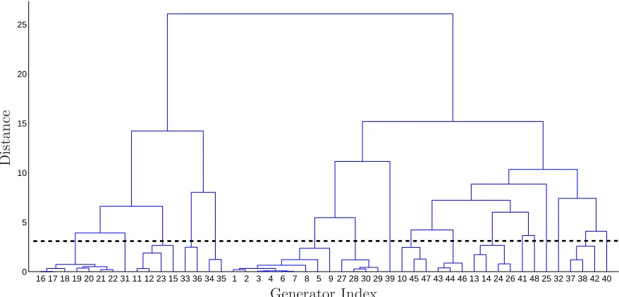
16 17 18 19 20 21 22 31 11 12 23 15 33 36 34 35 1 2 3 4 6 7 8 5 9 27 28 30 29 39 10 45 47 43 44 46 13 14 24 26 41 48 25 32 37 38 42 40 0
5 10 15 20 25
Generator Index
D
is
t
an
c
e
Figure 2.3: PCA-based generator clustering results using their rotor angles
The next step is to identify the coherent groups of the generators. For this, we use the PCA method, and MATLAB clustering routinelinkage. Fig. 2.3 shows the resulting clustering. In this figure, the horizontal represents the generator index, and the vertical axis represents the euclidean distance between the generator groups obtained by considering the three largest principle components of matrix T as defined in [30]. From this figure, different clustering partitioning can be obtained. Here we considered 17 areas as marked in Fig. 2.3 by setting the clustering distance to be equal to 3.
We then form the estimate of the center of inertia ∆ˆδkcoi(t) for areak,k= 1, . . . ,17 using (2.9). Based on the earlier discussion in Section 2.2, ∆ˆδcoik (t) is set equal to ∆ˆδks(t).
2.4.2 Identification using modal decomposition
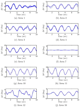
We next take a different approach for constructing ∆ˆδks(t) as outlined in Section 2.3. We first assume that the area partitioning that was obtained in the Section 2.4.1 is already given. The initial assignment of PMUs also satisfy the condition of the availability of at least one PMU per area as shown in Table 2.1. If area k contains only a single machine i, namely
2 4 6 8 10 −2 0 2 ∆ δ (d eg ) Time (sec)
(a) Area 1
2 4 6 8 10 −5 0 5 ∆ δ (d eg ) Time (sec)
(b) Area 2
2 4 6 8 10 −10 0 10 ∆ δ (d eg ) Time (sec)
(c) Area 3
2 4 6 8 10 −5 0 5 ∆ δ (d eg ) Time (sec)
(d) Area 4
2 4 6 8 10 −10 0 10 ∆ δ (d eg ) Time (sec)
(e) Area 5
2 4 6 8 10 −5 0 5 ∆ δ (D eg ) Time (sec) (f) Area 7
2 4 6 8 10 −10 0 10 ∆ δ (D eg ) Time (sec) (g) Area 10
2 4 6 8 10 −10 0 10 ∆ δ (d eg ) Time (sec)
(h) Area 11
2 4 6 8 10 −5 0 5 ∆ δ (D eg ) Time (sec) (i) Area 12
2 4 6 8 10 −5 0 5 ∆ δ (D eg ) Time (sec) (j) Area 16
11
1 3
2
12 4
7 15
17
16 9
14 13
10
6 8
5
Figure 2.5: The topology of the identified reduced-order system in Case 1
k= 6,8,9,13,14,15,17, we set ∆ˆδks(t) equal to the ∆ˆδi(t). For areas 1 and 5, there were two PMUs available per area. Therefore, we first form the approximate center of inertia from (2.13) using the available set of measurements, and then we extract their slow part and set them equal to ∆ˆδ1s(t) and ∆ˆδ6s(t). For the remaining areas, we extract the slow components ∆ˆδi(t) using Prony and set it equal to ∆ˆδsk, for machine ibelongs to area k. The details of this modal extraction is shown in Table 2.2. We then use the extracted slow components ∆ˆδs(t) to estimate
As. In the following section we compare the reduced-order model of the NPCC obtained using
Table 2.1: PMUs placed per area
Area Bus # Gen # Area Bus # Gen #
1 21,24 2,6 10 91 33
2 134 45 11 92 35
3 53 15 12 115 37
4 50 13 13 120 39
5 54,54 17,18 14 121 40
6 71 25 15 122 41
7 78 27 16 133 44
8 101 31 17 139 48
model-based reduction with Case 1 and Case 2 reduced-order models.
Table 2.2: Post-fault oscillatory modes of the ∆ˆδs
i(t) for the NPCC 48-machine in the frequency range [0.1, 1] Hz obtained from Prony
Mode # Eigenvalue Freq. (Hz) Damp. (%) 1
2 3 4 5 6 7 8
−0.0001±j1.6200 −0.0034±j2.3874 −0.0007±j2.9163 −0.6744±j3.4899 −0.0409±j3.7405 −0.0095±j4.4182 −0.0093±j5.1800 −0.0124±j5.9288
0.2578 0.3800 0.4641 0.5554 0.5953 0.7032 0.8244 0.9436
0.0062 0.1424 0.0240 19.3243
1.0934 0.2150 0.1795 0.2091
2.4.3 Validating the results
We next validate the identified reduced-order models of Case 1 and Case 2 by comparing their response with the responses of the actual system and the model-based reduced-order system to the same initial condition. Fig. 2.6 shows the trajectories of ∆δcoik (t) compared with ∆δsk(t) obtained from the reduced-order models, for a selected set ofk. Visually inspecting the trajectories in Fig. 2.6 verifies that the proposed measurement-based approaches of Case 1 and Case 2 result in better approximations of the full-order model compared to the model-based reduction. In order to quantify the differences in responses, we use the following metric as introduced in [26]:
Ja(k) = 1
tm−t1
Z tm
t1
|∆δk,sreduced(t)−∆δk,sactual(t)|dt. (2.16)
0 5 10 15 −3 −2 −1 0 1 2 3 Time (sec) (d e g )
∆δCOI 1 ∆δ
s
1model-based
(a)
0 5 10 15 −3 −2 −1 0 1 2 3 Time (sec) (d e g )
∆δCOI 1 ∆δ
s 1Case 1
(b)
0 5 10 15 −3 −2 −1 0 1 2 3 Time (sec) (d e g )
∆δCOI 1 ∆δ
s
1Case 2
(c)
0 5 10 15 −10 −5 0 5 10 Time (sec) (d e g )
∆δCOI
8 ∆δ
s
8model-based
(d)
0 5 10 15 −10 −5 0 5 10 Time (sec) (d e g )
∆δCOI
8 ∆δ
s
8Case 1
(e)
0 5 10 15 −10 −5 0 5 10 Time (sec) (d e g )
∆δCOI
8 ∆δ
s 8Case 2
(f)
0 5 10 15 −6 −4 −2 0 2 4 6 Time (sec) (d e g )
∆δCOI 17 ∆δ
s
17model-based
(g)
0 5 10 15 −6 −4 −2 0 2 4 6 Time (sec) (d e g )
∆δCOI 17 ∆δ
s
17Case 1
(h)
0 5 10 15 −6 −4 −2 0 2 4 6 Time (sec) (d e g )
∆δCOI
17 ∆δ
s 17Case 2
(i)
expected because of the more number of PMUs are assumed in Case 1.
Table 2.3: The calculated values of the error termJa(k) as defined in (2.16) using the model-based reduction, Case 1, and Case 2. Note that the trajectory of area 7 is the reference angle and it is zero by assumption.
Area (k) Model-based
Case 1 Case 2
1 0.2414 0.0777 0.1138
2 0.2854 0.1852 0.2424
3 0.8514 0.1087 0.4393
4 0.5328 0.1044 0.2450
5 0.6976 0.3008 0.2947
6 0.5856 0.1738 0.2445
7 0 0 0
8 1.9563 0.1787 0.2538
9 0.5005 0.2240 0.2292
10 1.1111 0.2907 0.5887 11 1.3260 0.1654 0.3394 12 0.3897 0.2476 0.3735 13 0.3858 0.3794 0.3739 14 0.4606 0.2246 0.2490 15 0.3746 0.2448 0.2929 16 0.1984 0.1142 0.1282 17 0.3261 0.1990 0.1935 Total 10.2232 3.2191 4.6017
Table 2.4 compares the frequency of the 9 slowest modes of the full-order model with the reduced-order models. It shows that both model-based reduction and the measurement-based reduction preserve the accuracy of the mode frequencies.
2.5
Conclusions
Table 2.4: The inter-area modes of the reduced-order systems compared with the full-order model
Full Model Reduced-Order
Model-Based Case 1 Case 2
Frequency Frequency Error(%) Frequency Error(%) Frequency Error(%)
(Hz) (Hz) (Hz) (Hz)
0.2567 0.2567 0.0272 0.2559 0.2901 0.2575 0.3387
0.3804 0.3815 0.2886 0.3810 0.1508 0.3802 0.0538
0.4661 0.4669 0.1660 0.4637 0.5093 0.4638 0.4880
0.5317 0.5342 0.4710 0.5320 0.0637 0.5276 0.7758
0.6009 0.6112 1.7179 0.6027 0.2940 0.6043 0.5646
0.6985 0.6990 0.0770 0.7021 0.5241 0.6993 0.1251
0.7201 0.7307 1.4611 — — — —
0.8264 — — 0.8216 0.5791 0.7899 4.4266
0.9093 0.9099 0.0594 0.9138 0.4896 0.9148 0.6082
Chapter 3
Identification of DAE Equivalent
Models of Power Systems
result of which the model was identified directly in the Kron-reduced form. In other words, the identity of every bus in the full-order model was lost in the reduced-order model. Such a loss is permissible if one wants to compute the oscillation modes, i.e., the eigenvalues of the state matrix, or to assess small-signal stability. These models, however, are not very suitable for the purpose of controller design since there is no well-defined way to implement a controller in the real system from a reduced-order model that does not preserve the bus identities.
In Chapter 3 we bridge this gap by proposing an alternative algorithm that identifies dynamic equivalent models while preserving the identities of a specific set of buses from the original system. The identified model, unlike Chapter 2, is in the form of a structured electric circuit described by nonlinear differential-algebraic equations (DAE). We consider the original network to be divided into r non-overlapping coherent areas. Each Areak is characterized by a unique set ofmk generators and a unique set of nk buses. A subset of these nk buses, referred to as
boundary buses, is defined as the set of all buses in Areak that are the end-points of tie-lines connecting this area to buses outside this area. Under the assumption of coherency, we consider every variable in the original network to exhibit a time-scale separation similar to Chapter 2. We first aggregate the boundary buses of every area to form a single equivalentpilotbus, whose voltages and injected currents can be calculated from the PMUs installed at the boundary buses. Using a modal decomposition method, we extract the slow time-scale components of these voltages and currents, and use them to identify the parameters of the reduced-order DAE model via least-squares. It should be noted that unlike Chapter 2, where our goal was to identify the small-signal model, the circuit representation of the equivalent model here forces us to retain the nonlinearity of the generator dynamics. We also add a brief discussion on how the identified DAE model can be used for designing Static VAR Compensators (SVC) to damp inter-area oscillations, and how this controller can be finally mapped back to the full-order network for implementation [38].
identification in details. Sections 3.3 and 3.4 illustrate the results through two case studies. Section 3.5 concludes the chapter.
3.1
Problem Formulation
Consider a power system network consisting of ngenerator buses andnl load buses connected by a given topology. Assume buses 1 through n to be the generator buses and buses n+ 1 throughn+nl to be the load buses. The electromechanical swing equations for theith generator,
i= 1, . . . , n,are given as:
˙
δi(t) =ωs(ωi(t)−1) (3.1a)
Miω˙i(t) =Pmi−Pei(t)−Di(ωi(t)−1), (3.1b)
where,
Pe0i(t) +Pi(t)−PLi(t) = 0, Q
0
ei(t) +Qi(t)−QLi(t) = 0, Pj(t)−PLj(t) = 0, Qj(t)−QLj(t) = 0,
(3.2)
fori= 1, . . . , nandj=n+ 1, . . . , n+nl. Here,δi(t),ωi(t),Mi,Di,Pmi,Pei(t),Qei(t) denote the
internal angle, speed, inertia, damping, mechanical power, active and reactive electrical powers produced by the ith generator, respectively.P0
ei(t) andQ
0
ei(t) denote the delivered active and
reactive powers from theith generator to theith bus. (Pk(t),Qk(t)) and (PLk(t),QLk(t)) denote,
respectively, the total active and reactive powers injected to thekth bus from other buses of the network, and the active and reactive powers of the loads at the kth bus, fork= 1, . . . , n+nl. Let S denote a set of bus indices where PMUs are placed so that the output equation can be written as
Here, ˜Vi(t),Vi(t)∠θi(t) denotes the voltage of theith bus, ˜Ii,j(t),Ii,j(t)∠φi,j(t) denotes the current injecting to the ith bus through the tie-line connecting busesiand j, and Ni is the set of all buses that are connected to the ith bus. All of these quantities are available over time when a PMU is installed at the ith bus.
The network is divided into r non-overlapping coherent areas. Each Areakis characterized by a unique set of mk generators and a unique set of nk buses. A subset of thesenk buses, are referred to as boundary buses if any tie-line radiating from these buses connects Areakto a bus that does not belong to Areak. This set is denoted by Bk. For our problem of interest we need the boundary buses of all areas to be equipped with PMUs. Hence, from this point onward we assume
S= r
[
k=1
Bk. (3.4)
In the reduced-order representation of this r-area network, each set of boundary buses Bk,
k= 1, . . . , r, are reduced to a single bus, referred to as a pilot bus of Area k. Assuming all the generators in each area to be coherent, this area is represented by a single equivalent generator behind thekth pilot bus. Thekth equivalent generator is modeled by an equivalent DAE similar to (3.1) as:
˙
δks(t) =ωs(ωsk(t)−1), (3.5a)
Mksω˙ks(t) =Pmsk−Pesk(t)−Dsk(ωks(t)−1), (3.5b)
where
Pe0sk(t) +Pks(t)−PLsk(t) = 0, Q0esk(t) +Qsk(t)−QsLk(t) = 0,
for k = 1, . . . , r. - Here, δks(t), ωks(t), Mks,Dsk,Pms k,P
s ek(t), Q
s
`
Area 1
Area 2 Area 3
Area 4
(a) A 4-area transmission network
1
s
G
2
s
G
3
s
G
4s
G
1
s p
V
2
s p
V
3
s p
V
4
s p
V
1
s p
I
2
s p
I
3
s p
I
4
s p
I
(b) The equivalent structured reduced-order network
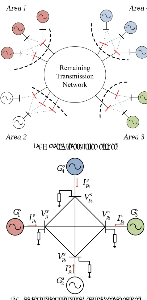
Figure 3.1: The reduction taking place in Chapter 3
speed, inertia, damping, mechanical power, active and reactive electrical power produced by the
kth equivalent generator, respectively,Pe0sk(t) andQ0esk(t) are the delivered active and reactive powers from the kth generator to thekth pilot bus,Pks(t), Qsk(t), PLs
j(t) and Q
s
the total active and reactive powers injected to the kth pilot bus from other pilot buses of the network, and the active and reactive powers of the loads at thekth pilot bus, respectively.
For example, consider the 4-area power system in Fig. 3.1a. The buses shown in red in each area denote their boundary buses. The structured reduced-order model of this network is shown in Fig. 3.1b. In this figure, the buses belonging to B1,B2, B3, and B4 are reduced to single
equivalent pilot buses representing Areas 1, 2, 3, and 4, respectively.Gs1,Gs2,Gs3, andGs4 are the respective equivalent generators whose models are given by (3.5).
Thekthgenerator is assumed to be connected to its respective pilot bus through an equivalent impedance (rsk+jx0ds
k). The voltage and injected current from the generator to the k
th pilot bus are denoted by ˜Vpsk(t) and ˜Ipsk(t), respectively, whose precise definition will be given in Section 3.2. Note that the identity of the boundary bus sets Bk,k= 1, . . . , r, are preserved in the reduced-order model. The actual transmission network connecting the boundary buses in Fig. 3.1a may be very complicated, but in the reduced-order network thejth and kth pair of pilot buses are connected by an equivalent tie-line with impedancezsjk =rsjk+jxsjk as shown in Fig. 3.1b. The main problem to be solved can then be stated as follows:
Consider S to be defined as in (3.4). Using the measured values of yi(t) in (3.3) available
from PMUs following a disturbance, sampled at time t=t0, t1, . . . , tm, estimate zjks , rsk, x
0s
dk, Mks, Dsk for all j, k∈ {1, . . . , r}.
We solve this problem using the four steps described in Section 3.2.
3.1.1 Comparison with Chapter 2
In Chapter 2, we linearized (3.1) and considered the Kron-reduced version of Fig. 3.1a, whereGs1
(3.5) instead of small-signal quantities (∆δsk(t),∆ωks(t)), k= 1, . . . , r as used in Chapter 2.
3.2
The Proposed Structured-Identification Approach
Step 1–Constructing an equivalent pilot bus for each area
The first step in constructing the structured equivalent network is to aggregate the boundary buses inBk to form an equivalent pilot bus. The criteria that was considered for this reduction is that the net injecting current/power to this equivalent pilot bus should be equal to the summation of the currents/powers injecting to the individual boundary buses belonging to Bk. Therefore, the total injected current and the voltage phasors of Bk, denoted respectively by
˜
Ipk(t) and ˜Vpk(t), are defined as follows:
˜
Ipk(t),Ipk(t)∠φpk(t) =
X
i∈Bk
˜
Ii(t), (3.6a)
˜
Vpk(t),Vpk(t)∠θpk(t) =
P
i∈Bk
˜
Vi(t) ˜Ii∗(t) ˜
I∗ pk(t)
, (3.6b)
where,
˜
Ii(t) = X
j∈Areak, j∈Ni
˜
Ii,j(t). (3.7)
The idea is shown in Fig. 3.2. We next describe how to find the pilot bus voltages and currents ( ˜Vpsk(t),I˜psk(t)), by extracting the slow time-scale motions of ( ˜Vpk(t),I˜pk(t)).
Step 2–Extracting (V˜psk(t),I˜psk(t)) from ( ˜Vpk(t),Ip˜k(t))
φpk(t) from (3.6), we will next construct their respective slow time-scale motions using modal
decomposition techniques.
As shown in [39], the Normal Form solution ofδi(t),i= 1, . . . , n, from the nonlinear model (3.1) is as follows:
δi(t)≈
2n
X
l=1
ρjleλlt+
2n
X
k=1 2n
X
l=1
ρ0jkle(λl+λk)t, (3.8)
where λl,l= 1, . . . ,2n, are the eigenvalues ofA, i.e., the linearized state matrix of (3.1), and the coefficients ρlk andρ0ijk denote the residues of the first-order and second-order modes of
δi(t). Let us sortλi based on the magnitude of their frequencies (i.e., imaginary part) as:
|Im(λ1)| ≤ |Im(λ2)| ≤ · · · ≤ |Im(λ2n)|.
From the assumption of the coherency, it follows that the modal content of theδs
i(t) from the nonlinear model (3.5) will be given in terms ofλl,l= 1, . . . ,2r. Hence, we may write:
δis(t)≈
2r
X
l=1
ρjleλlt+
2r
X
k=1 2r
X
l=1
ρ0jkle(λl+λk)t, (3.9)
SinceVps
k(t) is one of the outputs of the state space model of (3.5), its modal decomposition can
Coherent
Area k Coherent Area k
k
p
V
k
p
I
PMUPMU
PMU
Coherent Area k
k
s p
V
k
s p
I
Step 1 Step 2
be written as:
Vpsk(t) =
2r
X
l=1
αlkeλlt+
2r
X
i=1 2r
X
j=1
α0ijke(λi+λj)t, (3.10)
where the coefficients αlk and α0ijk denote the residues of the first-order and second-order modes of Vpsk(t). Now, if Vpk(t) is passed through a modal decomposition algorithm such as
Prony [24, 40], its linear fit can be estimated as
ˆ
Vpk(t) =
N
X
l=1
βlkeγlt, (3.11)
where N is the number of columns of the Hankel matrix indicating the number of identified modes. The values ofβlk andγl, forl= 1, . . . , N, will follow from the least squares estimation step of the Prony algorithm. Assuming an upper and lower bound for the frequencies of slow time-scale motion (0.1 Hz and 1 Hz in our simulations), we retain only those modal components in (3.11) whose frequencies fall within the selected band. The sum of these selected modal components are classified as ˆVpsk(t). Comparing with (3.10), this means that if the sum of two slow mode frequencies, whose individual values are not known in reality, exceeds the selected upper bound (1 Hz) or fall below the lower bound (0.1 Hz), the modal component resulting from that sum is not counted in constructing ˆVps
k(t). The estimates of the slow time-scale components
ofθpk(t),Ipk(t), andφpk(t), denoted respectively by ˆθ
s pk(t), ˆI
s
pk(t), and ˆφ
s
pk(t) can be constructed
similarly. Fig. 3.2 shows the use of these slow components to construct the variables at thekth
Step 3–Estimation of inter-area parameters
As mentioned earlier, each area is modeled with an equivalent classical generator with parameters including the transient reactance x0s
dk, the equivalent inertia M
s
k, and the equivalent mechanical dampingDsk. We also add an equivalent resistancerks in order to increase the model accuracy. We next discuss how to estimate these parameters in two separate steps; first, estimating x0ds
k
and rks; second, estimatingMks and Dks using a nonlinear least squares formulation (Step 3.2).
Step 3.1–Estimation of x0ds
k and r
s
k Fig. 3.3 shows the equivalent circuit connecting Gsk to thekth pilot bus. Applying the Ohm’s Law to this circuit, at any time tyields:
Eks(t)∠δks(t) = (rks+jx0ds k) ˜I
s
pk(t) + ˜V
s
pk(t). (3.12)
For all measurement instances t0, . . . , tm, we define the following quantities:
Φ0,|(rsk+jx0dsk)( ˆI
s
pk(t0)∠φˆ
s
pk(t0)) + ˆV
s
pk(t0)∠θˆ
s pk(t0)|,
.. .
Φm,|(rsk+jx0dsk)( ˆIpsk(tm)∠φˆspk(tm)) + ˆVpsk(tm)∠θˆpsk(tm)|.
Since Es
k(t) in (3.12) is constant over time, the estimation ofrsk and x0dsk can be posed as the
following nonlinear least squares problem [42]:
min x0s
dk, rsk
var Φ0, . . . ,Φm
, (3.13)
where var(·) represents the variance function. Once the values of x0ds
k and r
s
k are estimated from (3.13), the estimates ofEks(t)∠δks(t) denoted by ˆEks(t)∠δˆsk(t) can be found from (3.12) for
s s
k k
E
k
s d
jx
k k k
s s s
p p p
V V k
s p
I
sk
r
the kthequivalent pilot bus
Figure 3.3: The equivalent model of a coherent area
Step 3.2–Estimation of Ms
k, Dks, and Pmsk We next propose the following nonlinear least
squares (NLS) problem in order to find the remaining equivalent intra-area parameters, i.e.,
Mk,Dk and Pmk, fork= 1, . . . , r:
min Ms
k,Dsk,Pmks
Z tm
t0
|δˆks(t)−δks(t, Mks, Dks, Pmsk)|2dt, (3.14)
where ˆδks(t) is available from Step 3.1. Since (3.14) is a local NLS problem forGsk,δks(t, Mks, Dks, Pmsk) may be constructed by solving (3.5) with Pesk(t) = Re ˆEks(t)∠δˆks(t) ˜Ipsk∗(t) at every time
t=t0, . . . , tm.
Step 4–Estimation of inter-area impedance zijs
We next estimate the inter-area admittances using the values of ˜Vpsk(t) and ˜Ipsk(t), k = 1, . . . , r, that are identified in Step 2. Let us define ˜Is(t) , col( ˆIpsk(t)∠φˆspk(t)) and ˜Vs(t) , col( ˆVpsk(t)∠θˆpsk(t)), k= 1, . . . , r. At any time t, ˜Vks(t) and ˜Iks(t) satisfy:
˜
Is(t) =YsV˜s(t), (3.15)
whereYsis the (r×r) admittance matrix for the network contained between therequivalent pilot buses in Fig. 3.1b. Considering the time instances of the PMU data samples to bet=t0, . . . , tm,
1 s G 2 s G 3 s G 2 2 2 6.4 0.2 s s s H D M 1 1 1 23.64 0.1 s s s H D M 3 3 3 3.01 0.3 s s s H D M
Figure 3.4: 9-Bus WECC Model
Ys
˜
Vs(t0) | · · · |V˜s(tm)
| {z }
˜
Vs
=
˜
Is(t0) | · · · |I˜s(tm)
| {z }
˜
Is
, (3.16)
where ˜Vs and ˜Is are (r×m) matrices known from Step 2. One can then estimate Ys by solving the following least squares problem:
min Ys kY
sV˜s−I˜sk2
F,
s.t. Ys = (Ys)T, (3.17)
where k.kF denotes the Frobenius norm of a matrix. The choice of the Frobenius norm is due to the fact that (YsV˜s−I˜s) is a matrix, not a vector. OnceYs is estimated, we can calculate the inter-area impedances aszsij =− 1
3.3
Case Study 1
We first apply the structured identification proposed in Section 3.2 to identify the equivalent DAE model of the 3-generator 9-bus WECC as shown in Fig. 3.4. Since this model is already a reduced-order model of the WECC [43], we do not need to extract the slow time-scale motions of voltage or current phasors as described in Steps 1 and 2. Buses 1, 2, and 3 are treated as the pilot buses and are equipped with PMUs. The classical models of the generators are considered. The inertias and damping factors of the generators are also indicated in Fig. 3.4. The PMU measurements are generated using Power System Toolbox (PST) nonlinear dynamics simulation routines simu. The sampling rate is considered to be 1/60 Hz. A three-phase fault is assumed to occur at the line connecting buses 6 and 7. The fault starts att= 0.1 sec, clears at bus 6 at
t= 0.15 sec and at bus 7 at t= 0.2 sec. We next describe Steps 3 and 4 of our identification method applied to this system.
3.3.1 Estimation of x0ds
k
Since the generators of this system are the equivalent generators, we skip Steps 1 and 2 of the identification method. We first estimate the values ofx0ds
k,k= 1,2,3, by solving (3.13) using
MATLAB fminconroutine. The first compartment of Table 3.1 shows the estimation results for the three generators compared to their actual value. This table verifies the accuracy of the estimation of x0ds
k fork= 1,2,3.
3.3.2 Estimation of inter-area parameters
Table 3.1: Estimation results of the generator parameters for the WECC model
Parameter Gs
1 Gs2 Gs3
x0ds Actual 0.0608 0.1198 0.1813
Estimated 0.0608 0.1198 0.1813
Hs Actual 23.64 6.4 3.01
Estimated 23.6738 6.4304 3.0282
Ds/Ms Actual 0.1 0.2 0.3
Estimated 0.0987 0.2025 0.3051
Pms Actual 0.716 1.63 0.85
Estimated 0.7161 1.6301 0.8501
3.3.3 Identification of inter-area impedances
Using the measurements of voltage and current phasors available at buses 1, 2, and 3, we next estimate the matrixYs using (3.17). The resulting Ys matrix is:
Ys =
1.1068−j4.6952 0.1676 +j2.2858 −0.0648 +j2.2483 0.1676 +j2.2858 1.1623−j2.8030 −0.0173 +j0.4051 −0.0648 +j2.2483 −0.0173 +j0.4051 0.5591−j2.4474
. (3.18)
From (3.18), we calculate the inter-area tie-line impedances as follows: z12 = −0.0319 +
j0.4352, z13= 0.0128 +j0.4444, z23= 0.1055 +j2.4641. It should be noted that the value ofr12
is negative. This happens due to the loads of the system, which are here modeled as constant impedance loads. This can be justified by setting the load to zero for the same system, and observing that all resistance values will be non-negative. The plot of the residual error for (3.18) is shown in Fig. 3.5. The error shown in this figure is the relative error of the LS formulation (3.17), which is calculated as
Error(t) = kY
sV˜s(t)−I˜s(t)k
2
kI˜s(t)k
2
. (3.19)
2 3 4 5 6 7 8 9 10 4
6 8 10 12
x 10−15
Time (sec)
E
rr
o
r
Figure 3.5: The relative error of the results in (3.18) calculated using (3.19)
10
8
25
26 28
29 9
31
39
18 17
27
24 12
35
11 13
30
2 34
36 37
38 3
5 4 7
20 19
23 33
32
1 16
15 14
21
22 6 PMU
PMU
G1
G10
G8
G3
G2 G
4
G5 G7
G9
G6
PMU
PMU
Area 1
Area 2
Area 3
Area 4
PMU
0 2 4 6 8 10 0.7
0.8 0.9 1 1.1
Time (sec)
V
(p
u
) VV1
30
V35
V16
V26
V31
0 2 4 6 8 10
−0.2 −0.1 0 0.1 0.2 0.3
Time (sec)
θ
(r
a
d
)
θ1 θ30 θ35 θ16 θ26 θ31
Figure 3.7: The trajectories ofViandθiat the buses with PMUs in IEEE 39-bus model.
3.4
Case Study 2
We next consider the IEEE 39-bus model divided into four areas as shown in Fig. 3.6. The model parameters are derived from [44]. The original system is modified by removing the line connecting buses 16 and 17. The generator partitioning is chosen based on the similarity of the angles and frequencies. As shown in Fig. 3.6, each area is characterized by a set of pilot buses. Area 1 only includes G1 and the pilot bus 1. Area 2 consists ofG2 andG3 with two pilot buses
30 and 35.G5–G8 belong to Area 3 with a single pilot bus 16. Finally, Area 4 includes G8–G10
1 2 3 4 5 6 7 1
1.02 1.04 1.06 1.08 1.1
Time (sec)
(p
u
)
Vpk ˆ
Vs pk
k= 4
k= 1
k= 3
k= 2
(a)
1 2 3 4 5 6 7
−0.2 −0.1 0 0.1 0.2
Time (sec)
(r
a
d
)
θp
k ˆ
θs pk
k= 3
k= 2
k= 4
k= 1
(b)
Figure 3.8: The actual and the slow components of the equivalent pilot buses for the IEEE 39-bus model obtained in Step 1.
sampling rate is considered to be 1/60 Hz.
Considering the structure of this network, we next show how to identify the structured topology of its reduced-order network based on the approach described in Section 3.2.
3.4.1 Calculating Vˆpsk(t)∠θˆpsk(t) and Iˆpsk(t)∠φˆspk(t) for Area k
We first aggregate the boundary buses of each area shown in Fig. 3.6 to form a single equivalent pilot bus as described in Step 1 of Section 3.2, and then calculate the values of ˜Vpk(t) and ˜Ipk(t)
in (3.6), fork= 1, . . . ,4. We next extract the slow components of ˜Vpk(t) and ˜Ipk(t). For this, we
use the Prony method, and we only retain the modes in the range of [0.1 1] Hz as discussed in Step 2 of Section 3.2. Table 3.2 lists the identified modes of ˜Vpk(t) and ˜Ipk(t) in this frequency
range. The eigenvalues shown in boldface belong to the set of first-order electromechanical modes. The remaining eigenvalues are either the higher-order modes or the excitation modes of the system. Fig. 3.8 compares Vpk(t) and θpk(t) with the resulting ˆV
s
pk(t) and ˆθ
s
pk(t). This
figure shows a very interesting observation that although the actual bus voltages ( ˜Vi(t),i∈S) have both fast and slow modes, the construction ofVpk(t) andθpk(t) as shown in (3.6b) has an
![Figure 2.1:The discrepency between the actual measurement from the prediction of the models, taken from [12]](https://thumb-us.123doks.com/thumbv2/123dok_us/1564844.1192313/18.612.149.487.176.385/figure-discrepency-actual-measurement-prediction-models-taken.webp)