INVESTIGATION
A Simple Method for Finding Explicit Analytic
Transition Densities of Diffusion Processes
with General Diploid Selection
Yun S. Song*,†,1and Matthias Steinrücken* *Department of Statistics, University of California, Berkeley, California 94720 and†Computer Science Division, University of California, Berkeley, California 94720
ABSTRACTThe transition density function of the Wright–Fisher diffusion describes the evolution of population-wide allele frequencies over time. This function has important practical applications in population genetics, butfinding an explicit formula under a general diploid selection model has remained a difficult open problem. In this article, we develop a new computational method to tackle this classic problem. Specifically, our method explicitlyfinds the eigenvalues and eigenfunctions of the diffusion generator associated with the Wright–Fisher diffusion with recurrent mutation and arbitrary diploid selection, thus allowing one to obtain an accurate spectral representation of the transition density function. Simplicity is one of the appealing features of our approach. Although our derivation involves somewhat advanced mathematical concepts, the resulting algorithm is quite simple and efficient, only involving standard linear algebra. Furthermore, unlike previous approaches based on perturbation, which is applicable only when the population-scaled selection coefficient is small, our method is nonperturbative and is valid for a broad range of parameter values. As a by-product of our work, we obtain the rate of convergence to the stationary distribution under mutation–selection balance.
D
IFFUSION processes, which are continuous-time Mar-kov processes with almost surely continuous sample paths, have been successfully applied in various population genetic analyses in the past. Examples include finding the stationary distribution of allele frequencies and approximat-ing fixation times and probabilities (see Karlin and Taylor 1981; Ewens 2004; Durrett 2008 for other applications of diffusion processes). This success is largely due to the fact that the diffusion approximation captures the key features of an evolutionary model while ignoring unimportant details, thereby arriving at a simpler process that facilitates compu-tation. However, when a reasonably complex model of evo-lution is considered, one is faced with unwieldy equations even under the diffusion approximation. In particular, for Wright–Fisher diffusions with general diploid selection,finding an explicit analytic transition density function, which characterizes the evolution of population-wide allele frequencies over time, has remained a challenging open problem. The diffusion theory allows one to write down
a partial differential equation (PDE) satisfied by the transi-tion density, but solving the PDE analytically has proved to be difficult.
The transition density has several practical applications, including the following: Recently, there has been growing interest in analyzing samples taken from the same or related populations at different time points. For example, such data arise from experimental evolution of model organisms in the laboratory (e.g., bacteria, see Lenski 2011), from viral/ phage populations (Shankarappa et al. 1999; Wichman
et al. 1999), or from ancient DNA (Hummel et al. 2005); see also Bollback et al. (2008) and references therein. In particular, the recent sequencing of Neanderthal (Green
et al. 2010) and Denisova (Reich et al. 2010) genomes should provide new opportunities for studying the evolution of allele frequencies over time, possibly under the influence of natural selection. In applying the diffusion process to study the evolution of the populations underlying such sam-ples, it is important tofind the transition density accurately. Bollbacket al.(2008) analyzed samples from multiple time points by using a hidden Markov model in which the hidden states are the population-wide allele frequencies. To approx-imate the evolution of the allele frequencies, they applied Copyright © 2012 by the Genetics Society of America
doi: 10.1534/genetics.111.136929
Manuscript received November 16, 2011; accepted for publication December 20, 2011
1Corresponding author: University of California, EECS Department, 683 Soda Hall
finite difference methods to obtain approximate numerical solutions to the PDE satisfied by the transition density. Finite difference methods were also employed by Gutenkunstet al.
(2009) to obtain numerical approximations of the transition density in Wright–Fisher diffusions with population sub-structure, which the authors applied to develop a useful tool for demographic inference. When employing such numerical methods, however, one needs to exercise caution in choos-ing appropriate discretization grid points. Which discretiza-tion is appropriate may depend strongly on the parameters (e.g., the selection coefficient) of the model, and it is difficult to predict a priori whether a particular discretization will produce accurate solutions. Also, in a numerical approach, note that the PDE needs to be solved afresh if the initial or the final frequency is changed. It would be useful to have a solution that is analytic in those variables.
Since the transition density of the Wright–Fisher diffu-sion with selection has practical applications,finding an ex-plicit formula has significant merit and several researchers have considered the problem. As detailed later in the text, the so-called spectral representation of the transition density can be found if the eigenvalues and eigenfunctions of the diffusion generator are known. Indeed, this is the approach taken by Kimura (1955a, 1957), first for a diallelic model with genic selection (i.e., the case with the dominance pa-rameterh= 1/2, as described shortly) and later for the case of complete dominant selection (i.e., withh= 1), assuming no recurrent mutation in both cases. More precisely, Kimura proposed perturbation expansions of the eigenvalues and eigenfunctions in powers of the population-scaled selection coefficients (defined more precisely later). Although this method is valid fors,1, the expansions fail to converge for ssubstantially.1 [say,s.10, which is not so unusual for adaptive alleles (Eyre-Walker and Keightley 2007)]. Fur-thermore, the perturbation expansion scheme described in Kimura’s work is not entirely transparent.
For aneutralparent-independent mutation model, an ex-plicit spectral representation of the transition density for the one-locus Wright–Fisher diffusion has been known for some time (Shimakura 1977; Griffiths 1979). Griffiths and Li (1983) and Tavaré (1984) showed that this spectral repre-sentation can be interpreted in terms of a stochastic process dual to the diffusion. The time dependency of the transition density is solely given through the probability distribution of this dual process (see Griffiths and Spanò 2010 for an over-view). Barbouret al.(2000) extended this duality approach to include a general selection model, but the transition rates of the dual process depend on the moments of the stationary distribution, and under selection these moments are difficult to compute (Donnelly et al. 2001). Hence, while being of theoretical interest, their method does not readily lead to efficient computation of the transition density.
In this article, we develop a new, simple computational method with which tofind analytic transition density func-tions of diallelic Wright–Fisher diffusions under recurrent mutation and arbitrary diploid selection. In contrast to the
aforementioned mathematical work based on duality, our method explicitlyfinds the eigenvalues and eigenfunctions of the diffusion generator associated with the diffusion, thus leading to an explicit spectral representation of the transi-tion density functransi-tion. Specifically, the eigenfunctions are found as a series of orthogonal functions. Although some-what advanced mathematical concepts are needed to derive the necessary system of equations, the resulting algorithm is quite simple to describe and easy to implement, involving only standard linear algebra. Furthermore, unlike previous approaches (Kimura 1955a, 1957) based on perturbation, which is applicable only when the population-scaled selec-tion coefficient s is small, our method is nonperturbative and is valid for a broad range of parameter values, including large values of sand an arbitrary dominance parameter h. As an application of our work, we obtain the rate of conver-gence to the stationary distribution under mutation–selection balance.
The rest of this article is organized as follows. We begin with a brief review of the Wright–Fisher diffusion and de-scribe the notion of spectral representation. Orthogonal pol-ynomials, which we extensively employ in our work, are also introduced. Then, we illustrate the key ideas behind our method in the simple case of genic selection and no recur-rent mutation. Afterward, we apply our method to the gen-eral case of arbitrary diploid selection and recurrent mutation and show how the results for the no-mutation case can be recovered as a special case. We then assess the per-formance of our method and end with discussions on possi-ble applications and extensions.
Background
In this section, we review useful facts about diffusion pro-cesses. In particular, we highlight some key properties satisfied by backward generators of one-dimensional diffusions. We also introduce the relevant orthogonal polynomials that we utilize in our method.
Wright–Fisher diffusions
We consider a Wright–Fisher diffusion process with two alleles, denotedA0andA1. The population-wide frequency
ofA1is denoted byx; hence, the frequency ofA0is 1 2x.
The genotype fitness scheme considered in this article is as follows:
Genotype: A0=A0 A0=A1 A1=A1
Relative fitness: 1 1þ2 h s 1þ2 s
We refer to the case with the dominance parameterh= 1/2 as genic selection. The population-scaled selection coeffi -cient is defined as s = 2Ns, where N corresponds to the diploid population size, which is assumed to remain con-stant over time. The rate of mutation fromA0toA1is given
by a= 4Nu01and fromA1to A0byb= 4Nu10, whereu01
(respectively,u10) denotes the per-generation probability of
Note that the genotypefitness scheme introduced above does not include the case in which the homozygotes have a relative fitness of 1 and the heterozygote has a relative
fitness unequal to 1. However, by choosings close to zero andhlarge, we can mimic such a scheme in our framework. More generally, it is straightforward to apply the technique developed in this article to a selection scheme in which the heterozygote has relativefitness 1 +s1and the homozygote
A1/A1has relativefitness 1 +s2. However, to conform to the
convention widely adopted in the literature, we use the above-mentioned parameterization of relativefitnesses.
Throughout, we use f to denote a twice continuously differentiable bounded function over [0,1]. The backward generatorL of a one-dimensional diffusion process on [0,1] with diffusion coefficientn2(x) and drift coefficientm(x) acts
onfas
LfðxÞ ¼1
2n
2ð xÞ @
2
@x2ff ðxÞg þmðxÞ @
@xff ðxÞg:
In the Wright–Fisher diffusion,n2(x) =x(12x). The
con-tribution tom(x) from selection is
2sx ð12xÞ ½xþh ð122 xÞ;
while the contribution from recurrent mutation is
1
2 ½a ð12xÞ2b x:
See Ewens (2004, Chap. 5.1) for a more detailed description.
Self-adjointness and the spectrum of a generator
LetL2([0,1],r) denote the space of real-valued functions on
[0,1] that are square integrable with respect to some real positive density r(x). We refer toras the weight function. Define the inner producth,iras
hf;gir¼
Z 1
0
fðxÞgðxÞrðxÞdx; (1)
forf,g2L2([0,1],r).
For a diffusion process with diffusion coefficient n2(x)
and drift coefficientm(x), thescaledensityj(x) is defined as
jðxÞ ¼exp
2
Z x
x0
2 m ðzÞ
n2 ðzÞ d z
; (2)
and the speeddensityp(x) is defined as
p ðxÞ ¼ g
n2 ðxÞ j ðxÞ; (3)
wheregis some positive constant andx0is an arbitrary state
in [0,1]. For the results derived in this article it is crucial to establish thatL isself-adjointwith respect top. To this end, let f, g 2 L2([0,1], p) satisfy appropriate boundary
condi-tions relevant to the boundary behavior of the correspond-ing diffusion. The diffusions considered in this article exhibit
exit, regular reflecting, or entrance boundaries. If 0 is an exit boundary, then the appropriate boundary condition is LimxY0 f(x) = 0. If 0 is either a regular reflecting or an
entrance boundary, the appropriate boundary condition is limxY0ð1=jðxÞÞðdfðxÞ=dxÞ ¼0:Similar boundary conditions
apply as x[1. See Durrett (2008) or Ewens (2004) for more details. For the diffusions considered in this article, their corresponding boundary conditions and integration by parts imply
hL f;gip ¼ hf;L gip;
thus establishing thatL is self-adjoint.
The key property (known as the spectral theorem) that we utilize in our work is the following: SupposeBandB9are eigenfunctions of L that satisfy the requisite boundary conditions of the diffusion process. If their eigenvalues L and L9 are distinct, then the self-adjointness of L (i.e., hB;L B9ip¼ hL B;B9ip) implieshB,B9ip= 0. Hence,
eigen-functions of L with distinct eigenvalues are orthogonal with respect to the weight functionp(x).
ThatL is a self-adjoint negative semidefinite differential operator implies that its eigenvalues are all real and non-positive. Furthermore, for many boundary conditions, in-cluding the ones considered in this article, solutions of
L B ðxÞ ¼2L B ðxÞ satisfying the requisite boundary con-ditions exist for countably many distinct values ofL. Thus, for the diffusion processes considered in this article, there is a unique sequence
0# L0,L1,L2,⋯;
with Ln/N asn/ N (Karlin and Taylor 1981, Chap.
15.13). These eigenvalues f2LngNn¼0 are called the “
spec-trum”ofL; and it can be shown that their associated eigen-functionsfBn ðxÞgNn¼0;which satisfy
L Bn ðxÞ ¼ 2Ln Bn ðxÞ;
form a basis ofL2([0,1],p).
Spectral representation of the transition density
For any subsetS3[0,1], the transition density function of a diffusion process is the functionp:ℝ$0·[0,1]·[0,1]/
ℝ$0such that
ℙ½Xt 2SjX0¼x ¼ Z
S
pðt;x;yÞdy:
The transition density p(t; x, y) satisfies the Kolmogorov backward equation
@p ðt;x;yÞ
@t ¼L p ðt;x;yÞ
¼1
2 n
2 ðxÞ @2
@x2 fp ðt;x;yÞg
þm ðxÞ @
and the appropriate boundary conditions, see Karlin and Taylor (1981, Chap. 15.5). Here, the differential operator
L is the backward generator of the diffusion and it acts onx.
Let {Bn(x)} be the eigenfunctions of L that satisfy the proper boundary conditions of the diffusion process. Further, let 2Ln denote the eigenvalue of Bn(x). Then,
fn ðt;xÞ ¼e2Ln t Bn ðxÞ satisfies the partial differential
equation
@fn ðt;xÞ
@t ¼L fn ðt;xÞ; (4)
and the requisite boundary conditions. Furthermore, since
L is a linear differential operator, a linear combination of
e2LntBnðxÞis also a solution to (4). The spectral
representa-tion ofp(t;x,y) is given by
p ðt;x;yÞ ¼X
N
n¼0
cn ðyÞ e2Ln t Bn ðxÞ;
where the coefficients cn(y) depend on y and are set to satisfy the initial condition. For p(0;x,y) =d(x2 y), the Dirac-delta distribution, we obtain
pðt;x;yÞ ¼X
N
n¼0
e2Ln t p ðyÞBnðxÞBnðyÞ
hBn;Bnip
; (5)
wherepis the speed density defined in (3) andh,ipis the
inner product defined in (1). See Karlin and Taylor (1981, Chap. 15.13) for further details and examples.
In summary, the transition density function of a diffusion process can be determined if the eigenvalues and the eigenfunctions of L are known. The orthogonal polyno-mials described in the following two subsections are such eigenfunctions for certain neutral Wright–Fisher diffusion processes, and we make extensive use of them in our work to solve the eigenvalue problem in the presence of selection. In practice, we do not need to sum over infinitely many terms in (5). Since Ln/N asn/N, the exponential
terme2Ln t will be negligibly small fornsufficiently large.
Hence, we can obtain accurate approximations ofp(t;x,y) for t.0 by summing overn from 0 to some reasonable
finite cutoff. In Empirical transition densities and station-ary distributions andRate of convergence to the stationary distribution we provide explicit examples illustrating this property.
Jacobi polynomials
An excellent treatise on orthogonal polynomials can be found in Szegö (1939) and a concise collection of related formulas can be found in Abramowitz and Stegun (1965, Chap. 22). Here, we briefly review some key facts about a particular type of classical orthogonal polynomials.
For z2 [21,1], the Jacobi polynomials Pnða;bÞ ðzÞ satisfy
the differential equation
12z2d 2f ðzÞ
dz2 þ ½b2a2ðaþbþ2Þz dfðzÞ
dz
þn ðnþaþbþ1Þ fðzÞ ¼0: (6)
Forfixeda,b. 21,fPnða;bÞ ðzÞgform an orthogonal system
with respect to the weight function (12z)a(1 +z)bon the
interval [21,1]. Since the domain and the parameters of
Pðna;bÞ ðzÞ are not suitable for our purpose, we define the
following modified Jacobi polynomials, for x 2 [0,1] and
a,b.0:
Rnða;bÞ ðxÞ ¼Pnðb21;a21Þ ð2x21Þ:
Griffiths and Spanò (2010) use a slightly different, although related, convention.
For x2 [0,1], the modified Jacobi polynomialsRnða;bÞ ðxÞ
satisfy the differential equation
x ð12xÞ d 2 f ðxÞ
dx2 þ ½a2ðaþbÞ x dfðxÞ
dx
þn ðnþaþb21Þ f ðxÞ ¼0; (7)
which follows immediately from (6). For fixed a, b . 0, fRðna;bÞ ðxÞg is an orthogonal system with respect to the
weight functionxa21(12x)b21on [0,1]. More precisely,
Z 1
0
Rnða;bÞ ðxÞ Rmða;bÞðxÞxa21ð12xÞb21 dx¼dn;mDn ða;bÞ;
(8)
wheredn,mdenotes the Kronecker delta and the coefficient
Dn(a,b) is defined as
Dn ða;bÞ ¼ GðnþaÞGðnþbÞ
ð2 nþaþb21Þ G ðnþaþb21Þ G ðnþ1Þ:
(9)
Furthermore, fRðna;bÞ ðxÞgform a complete basis of the
Hil-bert spaceL2([0,1],xa21(12x)b21).
For n $ 1, it can be shown that Rnða;bÞ ðxÞ satisfies the
recurrence relation
x Rðna;bÞ ðxÞ ¼
ðnþa21Þ ðnþb21Þ
ð2 nþaþb21Þ ð2 nþaþb22Þ R ða;bÞ
n21 ðxÞ
þ
1 22
b22a222 ðb2aÞ
2 ð2 nþaþbÞ ð2 nþaþb22Þ
Rðna;bÞ ðxÞ
þ ðnþ1Þ ðnþaþb21Þ ð2 nþaþbÞ ð2 nþaþb21Þ R
ða;bÞ
nþ1 ðxÞ;
(10)
while, for n= 0,
x Rða0;bÞ ðxÞ ¼ a aþb R
ða;bÞ 0 ðxÞ þ
1
aþb R ða;bÞ
1 ðxÞ: (11)
Also, note thatRð0a;bÞ ðxÞ[1. The above recurrence relations
Gegenbauer polynomials
The classical Gegenbauer polynomials are a special case of the classical Jacobi polynomials, namely Pðn1;1Þ ð2x21Þ. In
our work, we defineGn(x) as
Gn ðxÞ ¼ 2x ð12xÞ Pðn1;1Þ ð2x21Þ ¼ 2x ð12xÞ Rðn2;2Þ ðxÞ
and refer to them as modified Gegenbauer polynomials. The minus sign will prove convenient later. Using (7), it can be shown that Gn(x) satisfies the differential equation
x ð12xÞ d 2fðxÞ
dx2 þ ðnþ2Þ ðnþ1Þ fðxÞ ¼0: (12)
Further, {Gn(x)} form an orthogonal system of polynomials with respect to the weight functionx21(12x)21:
Z 1
0
Gn ðxÞ Gm ðxÞ x21 ð12xÞ21 dx¼dn;m ðnþ2nÞþ ð21nþ3Þ:
Using the completeness of the Jacobi polynomials, it can be shown that {Gn(x)} form a complete basis of L2([0,1],
x21(12x)21).
Forn$1,Gn(x) satisfies the recurrence relation
xGn ðxÞ ¼ nþ1
2 ð2nþ3Þ Gn21 ðxÞ þ 1 2 Gn ðxÞ
þ ðnþ1Þ ðnþ3Þ
2ðnþ2Þð2nþ3Þ Gnþ1 ðxÞ;
(13)
while, forn= 0,
x G0 ðxÞ ¼
1
2 G0 ðxÞ þ 1 4 G1 ðxÞ:
These relations follow from (10) and (11). Furthermore, we haveG0(x)[ 2x(12x).
Diffusions with Genic Selection and No Mutation
As described earlier, to obtain the spectral representation ofp
(t; x,y), we need to solve the eigenvalue problem for the diffusion generator. In this section, we illustrate the key ideas underlying our method by considering the simple case of no mutation and genic selection (h= 1/2), in which case the involved algebra simplifies significantly. Incidentally, the genic selection case has been considered by many other researchers in the past; for example, see Kimura (1955a, 1957), Etheridge and Griffiths (2009), and Griffiths (2003). The modified Gegenbauer polynomials introduced above will play an important role in this section. The case with both recurrent mutation and general diploid selection (i.e.,hnot necessarily equal to 1/2) is addressed in the next section.
Description of the main idea
LetL0denote the diffusion part of the backward generator:
L0fðxÞ ¼1
2 x ð12xÞ
@2
@x2 ff ðxÞg: (14)
As is well known (Kimura 1955a,b, 1957; Karlin and Taylor 1981), it follows from Equation 12 that the modified Gegen-bauer polynomialsGn(x) are eigenfunctions ofL0,
L0Gn ðxÞ ¼ 2ln Gn ðxÞ;
where
ln¼
nþ2 2
:
With genic selection, the full backward generator is
L f ðxÞ ¼1
2 x ð12xÞ
@2
@x2 ffðxÞg þs x ð12xÞ
@ @x ff ðxÞg:
(15)
The speed density corresponding to this diffusion process is
p ðxÞ ¼ e 2 s x
x ð12xÞ; (16)
where we usedx0= 0 andg= 1 in (2) and (3), respectively.
Our goal is to find the eigenfunctionsBn(x) and the as-sociated eigenvalues 2Lnof the full generatorL:
L Bn ðxÞ ¼ 2Ln Bn ðxÞ: (17)
As discussed inBackground,L is self-adjoint with respect to the weight function p(x), which implies that its eigenfunc-tions Bn(x) and Bm(x), forn6¼ m, are orthogonal with re-spect top(x);i.e.,
Z 1
0
Bn ðxÞ Bm ðxÞ p ðxÞ dx}dn;m;
wherep(x) is shown in (16). In addition to the eigenfunc-tions, there may exist other sets of functions that are orthog-onal with respect to the same weight function p(y). For example, consider
Hn ðxÞ ¼e2s x Gn ðxÞ: (18)
We can verify thatHn(x) andHm(x), forn6¼m, are orthog-onal with respect to the weight functionp(x):
R1
0Hn ðxÞ Hm ðxÞ p ðxÞ dx¼
R1
0Gn ðxÞ Gn ðxÞ x21 ð12xÞ21 dx
¼dn;m
nþ1
ðnþ2Þ ð2nþ3Þ:
However, by directly applying L to Hn(x), one can check that Hn(x) are not eigenfunctions of L. But, since both {Hn(x)} and {Bn(x)} are orthogonal with respect to the same weight function p(x), and {Hn(x)} form a basis of
L2([0,1],p), we can representBn(x) as a linear combination
Bn ðxÞ ¼ X
N
m¼0
un;m Hm ðxÞ; (19)
whereun,mare constants to be determined. In the absence of
mutation, states 0 and 1 are absorbing states (exit bound-aries), so, as discussed inBackground,Bn(x) must satisfy the boundary conditions limxY0Bn(x) = limx[1Bn(x) = 0. Indeed,
our proposed eigenfunctions satisfy those conditions since
Hm(0) =Hm(1) = 0 for allm$0. Now, one can show
L Hn ðxÞ ¼e2s x ½L0 Gn ðxÞ2Q ðx;sÞ Gn ðxÞ
¼ 2e2s x ½ln Gn ðxÞ þQ ðx;sÞ Gn ðxÞ; (20)
where
Q ðx;sÞ ¼1 2s
2
x ð12xÞ: (21)
For smalls, Kimura (1955a) employed an equation similar to (20) to obtain perturbation expansions in powers ofsfor the eigenvalues and the eigenfunctions of the forward dif-fusion generator. Here, we proceed along a different avenue. The key difference is that our approach is nonperturbative and that it is valid for all parameter values.
Using (20) together with (17) and (19), we obtain
XN
m¼0
un;m ½lmþQ ðx;sÞ Gm ðxÞ ¼Ln XN
m¼0
un;m Gm ðxÞ:
(22)
Now, form$0, (13) can be used to show
Qðx;sÞGmðxÞ ¼aðm22ÞGm22ðxÞ þamð0ÞGmðxÞ þamðþ2ÞGmþ2ðxÞ;
where
aðm22Þ¼ 2s2
1 8
m ðmþ1Þ
ð2mþ1Þ ð2mþ3Þ 1fm$2g;
aðm0Þ¼ þs2 1
4
ðmþ1Þ ðmþ2Þ
ð2mþ1Þ ð2mþ5Þ;
aðþm2Þ¼ 2s2
1 8
ðmþ1Þ ðmþ4Þ
ð2mþ3Þ ð2mþ5Þ:
(23)
In thefirst line of (23), 1{Y} denotes an indicator function
that is equal to 1 if statementYis true or 0 otherwise. For a nonnegative integerk, multiplying (22) byGk(x) and in-tegrating over [0,1] with respect to the weight function
x21(12x)21yields
lk un;kþað2 2Þ
kþ2 un;kþ2það 0Þ
k un;kþaðþ 2Þ
k22 un;k22¼Ln un;k;
(24)
where we defineaðþ222Þ¼a
ðþ2Þ
21 ¼0:Note that (24) specifies
a linear system of equations with un,0,un,1,un,2,. . ., as
variables.
Algorithm 1 (genic selection)
The eigenvalues and eigenfunctions of the backward gener-atorL (15) for the genic selection case can be obtained as follows. In matrix form, (24) can be written as
0 B B B B B B B B @
l0það00Þ 0 a
ð22Þ
2 0 0 ⋯
0 l1það10Þ 0 a
ð22Þ
3 0 ⋯
aðþ02Þ 0 l2það20Þ 0 a ð22Þ
4 ⋯
0 aðþ12Þ 0 l3það30Þ 0 ⋯
0 0 aðþ22Þ 0 l4það40Þ ⋯
⋮ ⋮ ⋮ ⋮ ⋮ ⋱ 1 C C C C C C C C A 0 B B B B B B @
un;0 un;1 un;2 un;3 un;4
⋮ 1 C C C C C C A
¼Ln
0 B B B B B B @
un;0 un;1 un;2 un;3 un;4
⋮ 1 C C C C C C A : (25)
Let M denote the infinite-dimensional matrix on the left hand side of (25). The key fact is that the eigenvalues Ln
ofMcorrespond to the eigenvalues ofL (up to a sign), and the associated eigenvectors un = (un,0, un,1,un,2,. . .) ofM
determine the eigenfunctions ofL via (19). Now, we con-sider a sequence of approximations by truncating (25). For a positive integer D, we let M[D] be an D-by-D matrix
obtained by taking thefirstDrows and thefirstDcolumns ofM, and letuðnDÞ¼ ðu½nD;0;u
½D n;1;. . .;u
½D
n;D21Þ. Then, we
approx-imate (25) by
M½D u½Dn ¼L½Dn u ½D n
and solve this finite-dimensional linear system to obtain eigenvalues L½nD and eigenvectors u½nD: This linear algebra
problem can be easily solved using standard software pack-ages such as Matlab, Mathematica, or the freely available LAPACK library (http://www.netlib.org/lapack/). We show inEmpirical ResultsthatL½nDandu½nD;m converge very rapidly
as the truncation levelDincreases.
The eigenvectorsu½nDcome in two types: Eitheru½nD;m ¼0
for allmeven oru½nD;m ¼0 for allmodd. In fact, the linear
system M½D u½D
n ¼L½nD u
½D
n can be decomposed into two
subsystems, one involving only the even rows and even columns of M[D] acting on un
,mfor modd, and the other
involving only the odd rows and odd columns ofM[D]
act-ing onun,mformeven. Hence, the eigenvalues and
eigen-vectors ofM[D], forD= 2D9, can be determined by solving
twoD9-dimensional linear systems.
In the case of genic selection with no recurrent mutation, the eigenfunctions Bn(x) of the backward generatorL are also known as the oblate spheroidal functions in mathemat-ical physics, and they have received considerable amounts of attention previously (e.g., see Stratton et al. 1941). Note that the algorithm presented in this section provides an
ef-ficient way to evaluate these functions, a problem that remained difficult in the past.
expansion, evaluation of the transition density for large selection coefficients involves combining quantities with substantially different orders of magnitude. Thus, to obtain accurate numer-ical values of the transition density under strong selection, the coefficientsu½nDmust be determined with high precision.
Diffusions with General Diploid Selection and Recurrent Mutation
In this section, we generalize the method developed in the previous section by incorporating recurrent mutation and general diploid selection into the diffusion process. The same overall strategy described above applies here as well. The main computational differences are that general diploid selection leads to more involved algebra and that, to handle recurrent mutation, we need to deal with general Jacobi polynomials instead of the modified Gegenbauer polynomials.
Neutral diffusion with recurrent mutation
For a neutral diallelic model with recurrent mutation, the backward generatorL 0 is given by
L0 fðxÞ ¼1 2 x ð12xÞ
@2
@x2 ff ðxÞg þ 1
2 ½a ð12xÞ2b x
@ @x ff ðxÞg:
(26)
See Backgroundfor the definitions of aandb. By appropri-ately choosing the constantsx0andgin (2) and (3), the speed
density corresponding to this diffusion can be defined as
p0 ðxÞ ¼xa21 ð12xÞb21; (27)
which is the unnormalized Beta distribution. It can be shown (see Karlin and Taylor 1981, Chap. 15.13, or compare with Equation 7) that the Jacobi polynomialsRðna;bÞ ðxÞare
eigen-functions of the backward generator L0 with eigenvalues
2lða;bÞ n , where
lðna;bÞ¼
1
2 n ðnþaþb21Þ: (28)
Furthermore, the Jacobi polynomials Rðna;bÞðxÞ form an
or-thogonal system with respect to the weight functionp0(x).
Under recurrent mutation, the diffusion exhibits either reg-ular or entrance boundaries (e.g., see Karlin and Taylor 1981, Chap. 15.6, Example 8). The respective conditions given in Background for x = 0 and x = 1 imply that the eigenfunctions u(x) ofL0 need to satisfy
lim
xY0x a @
@x ff ðxÞg ¼0 and limx[1ð12xÞ b @
@x ff ðxÞg ¼0;
and the modified Jacobi polynomials Rðna;bÞðxÞ obey these
conditions.
Adding general diploid selection
The backward generator of the diffusion process with recurrent mutation and general diploid selection is
L f ðxÞ ¼L0f ðxÞ þ2 s x ð12xÞ ½xþh ð122 xÞ @
@xff ðxÞg;
(29)
whereL0fðxÞis the selectively neutral part shown in (26).
With appropriate constants x0 and g in (2) and (3), the
speed density for this diffusion can be defined as
p ðxÞ ¼es ðxÞ p0 ðxÞ; (30)
where p0(x) is given in (27) and sð xÞ is the mean fitness
function given by
s ðxÞ ¼2 h s2 ð12xÞ xþ2 sx2¼2 s x ½xþ2 h ð12xÞ;
(31)
which simplifies to the linear function 2sxforh= 1/2. The discussion inBackgroundimplies that the full backward gen-eratorL is self-adjoint with respect to the weight function p(x), and that its eigenfunctions {Bn(x)} form an orthogonal system with respect to the same weight function. Now, if we defineKn(x) as
Kn ðxÞ ¼e2s ðxÞ=2 Rðna;bÞ ðxÞ; (32)
then (8) implies that {Kn(x)} is a complete system of orthog-onal functions with respect to the weight function p(x). However, by applying the generator L to Kn(x), one can show that Kn(x) is not an eigenfunction ofL. Rather, we obtain
L Kn ðxÞ ¼e2s ðxÞ=2
n
L0 Rðna;bÞ ðxÞ2Q ðx;a;b;s;hÞ Rnða;bÞ ðxÞ
o
¼2e2s ðxÞ=2 hlða;bÞ
n Rðna;bÞ ðxÞ þQ ðx;a;b;s;hÞ Rnða;bÞ ðxÞ
i ;
where Q(x;a,b,s,h) is the following degree-4 polynomial inx:
Q ðx;a;b;s;hÞ ¼s h aþ ½1þa2ð2þ3 aþbÞ h x2ð1þaþbÞ ð122 hÞ x2
þ2 s2 x ð12xÞ ðhþx22 hxÞ2:
(33)
For no recurrent mutation (a=b= 0) we get (12x)xs [1 2 2h + 2(h + x 22hx)2s], and for h = 1/2 (genic
selection), (33) reduces to a degree-2 polynomial:
1
2 fs ½2b xþa ð12xÞ þs
2 x ð12xÞg In the case of just
drift and genic selection, we obtain 1 2 s
2 x ð12xÞ as in
(21).
Again, {Bn(x)} and {Kn(x)} are orthogonal with respect to the same weight functionp(x), and {Kn(x)} form a basis ofL2([0,1],p), wherep is defined in (30). Hence, we pose
a representation for the eigenfunctions of the form
Bn ðxÞ ¼X
N
m¼0
wn;m Km ðxÞ ¼ XN
m¼0
wn;m e2s ðxÞ=2 Rðma;bÞ ðxÞ;
(34)
where wn,m are constants to be determined. It can be checked that Km ðxÞ ¼e2s ðxÞ=2 Rða;bÞ
satisfies the proper regular reflecting or entrance boundary conditions, and hence so doesBn(x).
Now, L BnðxÞ ¼ 2LnBnðxÞ implies the following alge-braic equation:
XN
m¼0 wn;m
h
lðma;bÞþQ ðx;a;b;s;hÞ
i
Rðma;bÞ ðxÞ ¼Ln
XN
m¼0
wn;m Rmða;bÞ ðxÞ:
(35)
Using (10), we can represent Q ðx;a;b;s;hÞ Rðna;bÞ ðxÞ as
afinite linear combination ofRðja;bÞ ðxÞ:
Q ðx;a;b;s;hÞ Rðma;bÞ ðxÞ ¼bðm24Þ Rmða2;b4Þ ðxÞ þb
ð23Þ
m Rðma2;b3Þ ðxÞ
þ⋯þbðþm3Þ Rmðaþ;b3Þ ðxÞ þb
ðþ4Þ
m Rðmaþ;b4Þ ðxÞ;
(36)
where the coefficientsbðmiÞare constants that depend onm,
a,b,s, andh.
For a nonnegative integerk, multiplying (35) byRðka;bÞ ðxÞ
and integrating over [0,1] with respect to the weight func-tionp0(x) yields
lðka;bÞ wn;kþbð2 4Þ
kþ4 wn;kþ4þbð2 3Þ
kþ3 wn;kþ3þ⋯þbðþ 3Þ k23 wn;k23
þbðþk244Þ wn;k24¼Ln wn;k;
(37)
where we definebðjiÞ¼0 ifj,0.
Algorithm 2 (recurrent mutation and general diploid selection)
We can now describe our algorithm for finding the eigen-values and eigenfunctions of the backward generatorL
de-fined in (29) for the case with recurrent mutation and general diploid selection. From (37), we arrive at a linear systemMwn=Lnwn, wherewn= (wn,0,wn,1,wn,2,. . .) is an
infinite-dimensional vector of variables andMis an infi nite-dimensional matrix given by
M¼ 0 B B B B B B B B B B B B B B @
lð0a;bÞþb
ð0Þ
0 b
ð21Þ
1 b
ð22Þ
2 b
ð23Þ
3 b
ð24Þ
4 0 0 ⋯
bðþ1Þ
0 lð a;bÞ
1 þbð 0Þ
1 bð2 1Þ
2 bð2 2Þ
3 bð2 3Þ
4 bð2 4Þ
5 0 ⋯
bðþ02Þ b
ðþ1Þ
1 l
ða;bÞ
2 þb
ð0Þ
2 b
ð21Þ
3 b
ð22Þ
4 b
ð23Þ
5 b
ð24Þ
6 ⋯
bðþ3Þ
0 bðþ 2Þ
1 bðþ 1Þ
2 lð a;bÞ
3 þbð 0Þ
3 bð2 1Þ
4 bð2 2Þ
5 bð2 3Þ
6 ⋯
bðþ04Þ b
ðþ3Þ
1 b
ðþ2Þ
2 b
ðþ1Þ
3 l
ða;bÞ
4 þb
ð0Þ
4 b
ð21Þ
5 b
ð22Þ
6 ⋯
0 bðþ14Þ bðþ
3Þ
2 bðþ 2Þ
3 bðþ 1Þ
4 lð a;bÞ
5 þbð 0Þ
5 bð2 1Þ
6 ⋯
0 0 bðþ24Þ b
ðþ3Þ
3 b
ðþ2Þ
4 b
ð1Þ
5 l
ða;bÞ
6 þb
ð0Þ
6 ⋯ ⋮ ⋮ ⋮ ⋮ ⋮ ⋮ ⋮ ⋱ 1 C C C C C C C C C C C C C C A
Closed-form formulas forbðmiÞcan be found easily using
sym-bolic computation software such as Mathematica. In the Ap-pendix, we provide a dynamic programming algorithm for computingbðmiÞwhich is useful for implementation in an
im-perative programming language such as C/C++. Ifh= 1/2,
bðm24Þ¼bð2
3Þ
m ¼bðþ
3Þ
m ¼bðþ
4Þ
m ¼0 for all m$ 0, and
there-fore only the innermostfive diagonals ofMwill be nonzero. As in Algorithm 1, we approximateMwn=Lnwnby afi
nite-dimensional truncated linear system
M½D w½Dn ¼L½Dn w ½D n ;
wherewðnDÞ¼ ðw½nD;0;w
½D
n;1;. . .;w
½D
n;D21ÞandM[D]is the
subma-trix ofMconsisting of itsfirstDrows and Dcolumns. This
finite-dimensional linear system can be easily solved to ob-tain the eigenvalues L½nDand the eigenvectorswn½DofM[D].
We show in Empirical Results thatL½nD and w½nD;m converge
very rapidly as the truncation levelDincreases.
Note that the same cautionary remark mentioned at the end of Algorithm 1 also applies here.
Special case: No recurrent mutation
Let L0 denote the diffusion generator defined in (14),
which can be obtained from (26) by setting a = b = 0. Since Rð0a;bÞ ðxÞ[1, it satisfies L0B ¼ 2lB with l = 0.
However, fora=b= 0, the boundaries are exit boundaries, and thereforeRð0a;bÞ ðxÞdoes not satisfy the requisite
bound-ary conditions. Furthermore, Rð1a;bÞ ðxÞ ¼bx2a ð12xÞ/0 asa,b/0, so it is not of interest. In contrast, forn$0,
Rðnaþ;b2Þ ðxÞconverges toGn(x) asa,b/0, and, as established
inBackground,Gn(x) satisfiesL0B ¼ 2lBwith l¼lðn0þ;02Þ
and satisfies the requisite boundary conditions fora=b= 0. In summary, as a,b/0, the first two modified Jacobi polynomials become irrelevant, while the rest converge to the appropriate eigenfunctions ofL 0. These facts have been
noticed before (e.g., see Griffiths and Spanò 2010), and they allow us to embed the model with no recurrent mutation conveniently into the model with recurrent mutation as de-scribed below.
Ifa=b= 0, letLnandwn= (wn,0,wn,1,. . .), respectively,
denote the eigenvalues and eigenvectors ofM9, the subma-trix ofMobtained by omitting thefirst two rows and thefirst two columns. DefiningKm ðxÞ:¼es ðxÞ=2 Gm ðxÞ(instead of
Equation 32) yields the eigenvaluesLnand the
eigenfunc-tionsBn(x) for the backward diffusion generator with a gen-eral diploid selection model but no recurrent mutation. Indeed, under genic selection (h = 1/2) anda =b = 0, one can show that bðm2þ42Þ¼b
ð23Þ
mþ2¼b
ð21Þ
mþ2¼b
ðþ1Þ
mþ2¼b
ðþ3Þ
mþ2¼
bðþmþ42Þ¼0, whileb
ð22Þ
mþ2 ¼a
ð22Þ
m ,bðm0þÞ2¼a
ð0Þ
m , andbðþmþ22Þ¼a
ðþ2Þ
m ,
whereaðjiÞare defined in (23). The casesa.0,b= 0 and
a= 0,b.0 can be treated along similar lines.
Empirical Results
In this section we study the convergence behavior of the eigenvalues and eigenvectors of the submatrix M[D] as its
dimensionD increases. Further, we show how the spectral representation of the transition density can be employed to characterize the convergence rate of the diffusion to statio-narity,i.e., mutation–selection equilibrium.
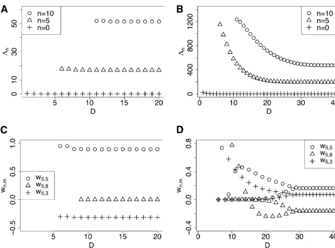
Convergence of the eigenvalues and eigenfunctions
As the dimensionDof the submatrixM[D]increases, we
gen-erally observe rapid convergence of the eigenvaluesL½nDand the entries w½nD;m of the eigenvectors, forfixedn,m,D. For
example, the convergence behavior ofL½0D;L½5D;L
½D
10 is shown
dominance parameterh= 1/2. Figure 1, A and B, illustrates that, for boths= 10 ands= 100,L½0Dconverges rapidly to 0 asDincreases, consistent with our expectation (see below). Thefigures illustrate that in generalL½nDconverges rapidly for a wide range ofsvalues, but that the convergence rate slows down as s increases. For a and b in biologically relevant ranges (say, 1023to 1021), we generally observe that
chang-ing the mutational parameters does not affect the conver-gence behavior significantly. Also, the dominance parameter
hhas little influence on the convergence rate provided that 0#h#1.
The typical convergence behavior of the eigenvector entries
w½nD;m is illustrated in Figure 1, C and D, fors= 10 ands= 100,
respectively. As Figure 1C shows, the rate of convergence is very fast for smalls. For larges, as in Figure 1D,w½nD;m mayfluctuate
for small values ofD, but they stabilize rapidly asDincreases. In general, we observe that the convergence of L½nD and that of
w½nD;m are roughly synchronized;i.e., for afixedn,Lnandw½ D
n;m
stabilize near similar values ofD.
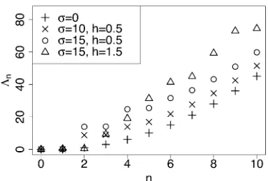
Figure 2 shows the dependence of L½nD ons,h, andn. Observe that L½nD increases rapidly as n increases, which
implies that using afinite number of terms in the spectral representation of the transition density should yield an ac-curate approximation of the true transition density. Increas-ing s or choosing h significantly different from 0.5 (the genic selection case) shifts the entire spectrum upward, but in all cases we observe thatL½nDincreases rapidly withn.
Empirical transition densities and stationary distributions
For given mutation and selection parameters, the eigenval-ues2Lnand the eigenfunctionsBn(x) found by our method
can be used to obtain the transition density via the spectral representation (5), for arbitraryt.0 andx,y2[0,1]. This
representation includes the stationary density, which admits a more explicit analytic form. To this end, note that a diffu-sion generator L maps constant functions to zero. In the case with recurrent mutation, we have either regular refl ect-ing or entrance boundaries, and constant functions actually satisfy the requisite boundary conditions. Hence, constant functions are valid eigenfunctions of L with eigenvalue zero. That is, L0 = 0 and B0(x) = C, where C is some
constant, for allx2[0,1]. Thus, the density of the stationary measure is given by
lim
t/Np ðt;x;yÞ ¼p ðyÞ
B0 ðxÞ B0 ðyÞ
hB0;B0ip
¼p ðyÞ C
2
hC;Cip
¼R1 p ðyÞ
0p ðzÞ d z ;
where p ðyÞ ¼es ðyÞ p
0 ðyÞ is the speed density defined in
(30). The integral in the denominator (which corresponds to a normalization constant for the stationary density) can be solved efficiently using our approach: SinceB0is a constant
function, we can express the integral as
Z 1
0
p ðzÞ d z¼ hB0;B0ip B0 ð1Þ B0 ð1Þ:
Then, using the representation
B0 ðxÞ ¼ XN
m¼0
w0;m e2s ðxÞ=2 Rðma;bÞ ðxÞ;
and the facts s ð1Þ ¼2 s [cf., (31)] and
Rðna;bÞ ð1Þ ¼G ðnþbÞ=½G ðnþ1Þ G ðbÞ, we obtain
Figure 1 Convergence of the eigenvaluesL½nD
and coefficientsw½nD;m with increasing truncation
levelD. The mutation rates are set toa¼b¼
0.01 and the dominance parameterh¼0.5. (A)
L0½D;L5½D;L½10Dfors¼10. (B)L½0D;L5½D;L½10Dfor
s ¼ 100. (C)w½5D;3;w5½D;5;w5½D;8 for s ¼ 10. (D)
R1
0p ðzÞ d z¼ PN
m¼0
w0;m 2
DRmða;bÞ;Rðma;bÞ E
p0
e2s ð1Þ h PN
k¼0w0;k Rkða;bÞ ð1Þ i2
¼
PN m¼0
w0;m
2
Dm ða;bÞ
e22s
PN
k¼0w0;k
G ðkþbÞ Gðkþ1Þ GðbÞ
2; (38)
where Dm(a,b) is the combinatorial coefficient defined in
(9). Thus, the integral can be evaluated purely algebraically. For a fixedn,wn,m/0 as m/N, so we can obtain an
accurate approximation of (38) by truncating the infinite sums and by computing w0,m using the method described
in this article. In special cases, the integralR01p ðzÞ d zcan be evaluated numerically using other methods (e.g., see Wakeley and Sargsyan 2009), but, for general s and h, standard numerical integration techniques do not seem to provide accurate answers.
Figure 3 shows some examples of the time evolution of the transition density function, with thet=Ncase corre-sponding to the stationary distribution. Specifically, three different types of selection schemes are illustrated:
1. Illustrated in Figure 3A are the densities forstrong posi-tive selection (s = 100, h = 0.5), when starting with a small initial frequency of x = 0.0005. As expected, for small t there is still some probability mass near 0, but already a substantial amount has moved to 1. At stationarity, the mass is concentrated at the boundaries, with the concentration near 1 being far more pronounced than that near 0.
2. Figure 3B shows the dynamics ofbalancing selection(s= 0.01, h = 10000), starting from initial frequency x = 0.0005. As time evolves, the mass gets shifted from the boundary at 0 to an intermediate frequency ofy= 0.5, where a large fraction of probability mass resides at stationarity.
3. In Figure 3C, the allele A1 exhibits weakly deleterious
selection (s =21, h= 0.5), with the initial frequency being x= 0.5. Initially most of the probability mass is concentrated around frequency y= 0.5. As the density evolves with time, it spreads out over the interval, and the peak of the density moves to lower frequencies. At stationarity, most of the mass is concentrated around the boundary at 0.
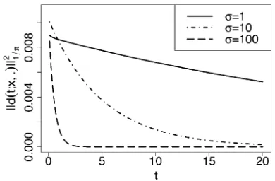
Rate of convergence to the stationary distribution
The spectral representation also allows us to obtain the rate of convergence to the stationary density. The differenced(t;
x,y) between the transition density and the stationary den-sity is given by
d ðt;x;yÞ:¼p ðt;x;yÞ2R1p ðyÞ 0p ðzÞ d z
¼XN n¼1
e2Ln t p ðyÞ Bn ðxÞ Bn ðyÞ hBn;Bnip :
Define kfk1=p¼
ffiffiffiffiffiffiffiffiffiffiffiffiffiffiffiffi
hf;fi1=p
q
. Then, by orthogonality of the eigenfunctions, we obtain
kdðt;x;Þk21=p¼
PN
n¼1e
22 Ln t½Bn ðxÞ2
hBn;Bnip
¼XN
n¼1
e22 Ln te
2s ðxÞ h PN
k¼0wn;k Rkða;bÞ ðxÞ i2
PN m¼0
wn;m
2
Dm ða;bÞ ; (39)
which can be approximated by truncating the infinite sums. Figure 4 shows the dependence of∥dðt;x;Þ∥21=pon timet, for
a = 0.01, b = 0.01, h = 0.5, s2{1,10,100}, and initial frequencyx= 0.0005. As expected, the distance to the sta-tionary distribution decreases over time, and the rate of convergence is faster for largers. We note that the spectral representation can also be readily employed to study con-vergence rates measured by other metrics such as the total variation distance or relative entropy.
Discussion
In this article, we developed a simple method for finding the eigenvalues and eigenfunctions of the diffusion gen-erator associated with the Wright–Fisher diffusion with recurrent mutation and general diploid selection. As de-scribed in Background, these eigenvalues and eigenfunc-tions can be used to construct a spectral representation (5) of the transition density. Since the eigenvalues 2Ln
tend to 2N as n / N, and the contribution of the nth eigenfunction to the transition density is proportional to
e2Ln t, we can truncate the series (5) at some appropriate
level and obtain a highly accurate approximation of the transition density. The mathematical derivation of our work invokes the theory of self-adjoint operators and or-thogonal functions, but the resulting algorithm involves only standard linear algebra, which is straightforward to
Figure 2 Magnitude of the eigenvalues {2Ln} of the diffusion generator L fora= 0.01,b= 0.01, and various values of the selection coefficients
implement. For a given set of parameters, computing the
first 500 eigenvalues and eigenfunctions using our method takes only a few seconds in Mathematica.
An accurate transition density enables one to estimate the parameters of Wright–Fisher diffusions, perhaps most inter-estingly the selection parameters. As mentioned in the In-troduction, Bollback et al. (2008) suggested a hidden Markov model framework for estimating the selection co-efficients by analyzing samples taken from multiple time points. The analytic transition density obtained from our method can be incorporated into that framework and thereby ameliorate potential numerical problems that may arise from trying to solve the Kolmogorov equation using discretization. Furthermore, our approach can be applied to devise an algebraic method for computing the sampling probability at stationarity under a general selection model.
There are several interesting extensions of our work to explore. It is known (Shimakura 1977; Griffiths 1979; Griffiths and Spanò 2010) that multivariate Jacobi polynomials, orthog-onal with respect to the Dirichlet distribution, are eigenfunc-tions of multiallelic diffusions under parent-independent mutation models. We believe that the technique developed in this article can be extended tofind the spectral representa-tion of the transirepresenta-tion density of a multiallelic diffusion with parent-independent mutation and general diploid selection.
For a neutral diallelic Wright–Fisher model with subdi-vided population structure, Lukić et al. (2011) recently obtained numerical approximations of the transition density by using a certain class of orthogonal polynomials. We re-mark that the orthogonal polynomials used in that approach are not eigenfunctions of the diffusion generator. Further, the system of ordinary differential equations (ODEs)
satis-fied by the coefficients of the basis functions does not admit a simple solution, so Lukić et al.(2011) employed afinite difference method with which to solve the ODEs
numeri-cally. Note that their method does not provide a proper spec-tral representation of the transition density, since it does not
find the eigenvalues and eigenfunctions of the diffusion gen-erator. It might be possible to extend the technique devel-oped in this article to obtain a spectral representation of the transition density in the case with subdivided population structure and general diploid selection.
In this article, we considered only one-locus Wright–Fisher diffusions. It is generally acknowledged that inference of evo-lutionary parameters, especially regarding selection, can be im-proved significantly by taking into account additional data at closely linked loci. Hence, it would be desirable to extend the approach described here to handle the dynamics of multilocus diffusions. However, our current technique relies on the fact that the eigenfunctions are known for the diffusion generator under neutrality. Therefore, to be able to apply our approach to multilocus diffusions with recombination and selection, one
Figure 3The transition density p(t;x,y) as a function ofy. Various times, selection param-eters, and initial frequencies were considered. The mutation rates were set toa=b= 0.01 in all examples. Thet=Ncase corresponds to the stationary distribution. A truncation level ofD= 1000 was used in the computation, and Equa-tions 5 and 34 were approximated by summing over 0#n#300 and 0#m#500. (A) Strong positive selection:s= 100,h= 0.5,x= 0.0005. (B) Balancing selection:s= 0.01,h= 10000,x= 0.0005. (C) Weakly deleterious selection:s = 21,h= 0.5,x= 0.5.
Figure 4 Convergence of the transition density to stationarity as time evolves, for initial frequencyx= 0.0005. Deviation from the stationary den-sity is measured by∥dðt;x;Þ∥2
1=p, defined in (39). The mutation and selection
would have to know the eigenfunctions in the neutral case. To our knowledge, no such eigenfunctions are known.
Since diffusion processes also arise in other disciplines (e.g., physics and mathematicalfinance), several approaches have been proposed to obtain efficient approximations of the transition densities for diffusions more general than the Wright–Fisher diffusion (see Srensen 2004; Aït-Sahalia 2008, for example). It would be interesting to investigate whether one could borrow techniques from those fields to the population genetics applications mentioned above.
Finally, we note that Mano (2009) recently employed the representation of the transition density given by Kimura (1955a) and the moment duality used in Barbour et al.
(2000) to investigate the dynamics of the number of line-ages in the ancestral selection graph dual to the Wright– Fisher diffusion. The representation of the transition density found in this article can be employed to include recurrent mutation into that framework.
Acknowledgments
We thank two reviewers for helpful comments and sugges-tions. This research is supported in part by National Institutes of Health grants R00-GM080099 and R01-GM094402 to Y.S.S. and Deutsche Forschungsgemeinschaft Research Fellowship STE 2011/1-1 to M.S.
Literature Cited
Abramowitz, M., and I. A. Stegun (Editors), 1965 Handbook of Mathematical Functions. Dover, New York.
Aït-Sahalia, Y., 2008 Closed-form likelihood expansions for mul-tivariate diffusions. Ann. Stat. 36(2): 906–937.
Barbour, A. D., S. N. Ethier, and R. C. Griffiths, 2000 A transition function expansion for a diffusion model with selection. Ann. Appl. Probab. 10: 123–162.
Bollback, J. P., T. L. York, and R. Nielsen, 2008 Estimation of 2Nes from temporal allele frequency data. Genetics 179: 497–502. Donnelly, P., M. Nordborg, and P. Joyce, 2001 Likelihoods and
simulation methods for a class of nonneutral population genet-ics models. Genetgenet-ics 159: 853–867.
Durrett, R., 2008 Probability Models for DNA Sequence Evolution. Springer, New York.
Etheridge, A. M., and R. C. Griffiths, 2009 A coalescent dual pro-cess in a moran model with genic selection. Theor. Popul. Biol. 75(4): 320–330.
Ewens, W. J., 2004 Mathematical Population Genetics: I. Theoret-ical Introduction. Springer, New York.
Eyre-Walker, A., and P. Keightley, 2007 The distribution offitness effects of new mutations. Nat. Rev. Genet. 8(8): 610–618. Green, R. E., J. Krause, A. W. Briggs, T. Maricic, U. Stenzelet al.,
2010 A draft sequence of the neandertal genome.Science328 (5979): 710–722.
Griffiths, R. C., 1979 A transition density expansion for a multi-allele diffusion model. Adv. Appl. Probab. 11: 310–325.
Griffiths, R. C., 2003 The frequency spectrum of a mutation, and its age, in a general diffusion model. Theor. Popul. Biol. 64(2): 241–251.
Griffiths, R. C., and W.-H. Li, 1983 Simulating allele frequencies in a population and the genetic differentiation of populations under mutation pressure. Theor. Popul. Biol. 23(1): 19–33. Griffiths, R. C., and D. Spanò, 2010 Diffusion processes and
co-alescent trees, pp. 358–375 inProbability and Mathematical Ge-netics: Papers in Honour of Sir John Kingman, Vol. 10, edited by N. H. Bingham, and C. M. Goldie. Cambridge University Press, Cambridge, UK.
Gutenkunst, R. N., R. D. Hernandez, S. H. Williamson, and C. D. Bustamante, 2009 Inferring the joint demographic history of multiple populations from multidimensional snp frequency data. PLoS Genet. 5(10): e1000695.
Hummel, S., D. Schmidt, B. Kremeyer, B. Herrmann, and M. Oppermann, 2005 Detection of the CCR5-D32 HIV resistance gene in bronze age skeletons. Genes Immun. 6(4): 371–374. Karlin, S., and H. Taylor, 1981 A Second Course in Stochastic
Pro-cesses. Academic Press, San Diego.
Kimura, M., 1955a Stochastic processes and distribution of gene frequencies under natural selection, pp. 33–53 inCold Spring Harbor Symposia on Quantitative Biology, Vol. 20. Cold Spring Harbor Laboratory Press, Cold Spring Harbor, NY.
Kimura, M., 1955b Solution of a process of random genetic drift with a continuous model. Proc. Natl. Acad. Sci. USA 41: 144–150. Kimura, M., 1957 Some problems of stochastic processes in
ge-netics. Ann. Math. Stat. 28(4): 882–901.
Lenski, R. E., 2011 TheE. colilong-term experimental evolution project site. Available at: http://myxo.css.msu.edu/ecoli. Ac-cessed: November, 2011.
Lukić, S., J. Hey, and K. Chen, 2011 Non-equilibrium allele frequency spectra via spectral methods. Theor. Popul. Biol. 79(4): 203–219. Mano, S., 2009 Duality, ancestral and diffusion processes in
mod-els with selection. Theor. Popul. Biol. 75(2–3): 164–175. Reich, D., R. E. Green, M. Kircher, J. Krause, N. Pattersonet al.,
2010 Genetic history of an archaic hominin group from Deni-sova Cave in Siberia. Nature 468(7327): 1053–1060.
Shankarappa, R., J. B. Margolick, S. J. Gange, A. G. Rodrigo, D. Upchurch et al., 1999 Consistent viral evolutionary changes associated with the progression of human immunodeficiency virus type 1 infection. J. Virol. 73(12): 10489–10502.
Shimakura, N., 1977 Equations différentielles provenant de la génétique des populations. Tohoku Math. J. 29: 287–318. Stratton, J. A., P. M. Morse, L. J. Chu, and R. A. Hutner, 1941 Eliptic
Cylinder and Spheroidal Wave functions. Wiley, New York. Szegö, G., 1939 Orthogonal Polynomials, Ed. 4th. American
Math-ematical Society, Providence, RI.
Srensen, H. 2004 Parametric inference for diffusion processes ob-served at discrete points in time: a survey. Int. Statist. Rev. 73 (3): 337–354.
Tavaré, S., 1984 Line-of-descent and genealogical processes, and their applications in population genetics models. Theor. Popul. Biol. 26: 119–164.
Wakeley, J., and O. Sargsyan, 2009 The conditional ancestral se-lection graph with strong balancing sese-lection. Theor. Popul. Biol. 75(4): 355–364.
Wichman, H. A., M. R. Badgett, L. A. Scott, C. M. Boulianne, and J. J. Bull, 1999 Different trajectories of parallel evolution during viral adaptation. Science 285(5426): 422–424.
Appendix
Here, we describe the computation of the coefficientsbðmiÞin Equation (36). Recall that the polynomialQ(x;a,b,s,h) defined
in (33) is of degree 4. Represent this polynomial as
Q ðx;a;b;s;hÞ ¼X 4
l¼0
qlxl; (40)
where ql are coefficients that depend on a, b, s, and h. As shown in (10) and (11), x Rmða;bÞ ðxÞ satisfies a three-term
recurrence relation of the form
x Rðma;bÞ ðxÞ ¼g ðm;m21Þ Rðma2;b1Þ ðxÞ þg ðm;mÞ R ða;bÞ
m ðxÞ
þg ðm;mþ1Þ Rmþða;b1Þ ðxÞ;
whereg(m,m21),g(m,m),g(m,m+1) are coefficients that depend onmanda,b. Note that (11) impliesg(0,21) = 0. Using the recurrence relation inductively gives
xlRðma;bÞ ðxÞ ¼ X mþl
k¼m2l
h ðm;l;kÞ Rkða;bÞ ðxÞ; (41)
where
h ðm;l;kÞ:¼
dm;k;
if l¼0;
1fjm212kj#l21g g ðm;m21Þ h ðm21;l21;kÞ
þ1fjm2kj#l21g g ðm;mÞ h ðm;l21;kÞ
þ1fjmþ12kj#l21g g ðm;mþ1Þ h ðmþ1;l21;kÞ;
if l.0:
8 > > > > > > < > > > > > > :
(42)
Now, (40) and (41) imply
Q ðx;a;b;s;hÞ Rðma;bÞ ðxÞ ¼ P4 l¼0
ql X mþl
k¼m2l
h ðm;l;kÞ Rkða;bÞ ðxÞ ¼ X mþ4
k¼m24 2 4 X4
l¼jk2mj
ql h ðm;l;kÞ 3
5 Rðka;bÞ ðxÞ:
Thus, the coefficientsbðmiÞin (36) are given by
bðiÞm ¼ X4
l¼jij
ql h ðm;l;kÞ;