University of Windsor University of Windsor
Scholarship at UWindsor
Scholarship at UWindsor
Electronic Theses and Dissertations Theses, Dissertations, and Major Papers
2008
Probabilistic three-dimensional object tracking based on adaptive
Probabilistic three-dimensional object tracking based on adaptive
depth segmentation
depth segmentation
Ehsan Parvizi University of Windsor
Follow this and additional works at: https://scholar.uwindsor.ca/etd
Recommended Citation Recommended Citation
Parvizi, Ehsan, "Probabilistic three-dimensional object tracking based on adaptive depth segmentation" (2008). Electronic Theses and Dissertations. 8234.
https://scholar.uwindsor.ca/etd/8234
This online database contains the full-text of PhD dissertations and Masters’ theses of University of Windsor students from 1954 forward. These documents are made available for personal study and research purposes only, in accordance with the Canadian Copyright Act and the Creative Commons license—CC BY-NC-ND (Attribution, Non-Commercial, No Derivative Works). Under this license, works must always be attributed to the copyright holder (original author), cannot be used for any commercial purposes, and may not be altered. Any other use would require the permission of the copyright holder. Students may inquire about withdrawing their dissertation and/or thesis from this database. For additional inquiries, please contact the repository administrator via email
NOTE TO USERS
This reproduction is the best copy available.
®
Probabilistic 3D Object Tracking Based
on Adaptive D e p t h Segmentation
by
Ehsan Parvizi
A Thesis
Submitted to the Faculty of Graduate Studies through Electrical and Computer Engineering in Partial Fulfillment of the Requirements for the Degree of Master of Applied Science at the
University of Windsor
1*1
Library and Archives CanadaPublished Heritage Branch
395 Wellington Street Ottawa ON K1A0N4 Canada
Bibliotheque et Archives Canada
Direction du
Patrimoine de I'edition
395, rue Wellington Ottawa ON K1A0N4 Canada
Your file Votre reference ISBN: 978-0-494-47082-4 Our file Notre reference ISBN: 978-0-494-47082-4
NOTICE:
The author has granted a non-exclusive license allowing Library and Archives Canada to reproduce, publish, archive, preserve, conserve, communicate to the public by
telecommunication or on the Internet, loan, distribute and sell theses
worldwide, for commercial or non-commercial purposes, in microform, paper, electronic and/or any other formats.
AVIS:
L'auteur a accorde une licence non exclusive permettant a la Bibliotheque et Archives Canada de reproduire, publier, archiver,
sauvegarder, conserver, transmettre au public par telecommunication ou par Plntemet, prefer, distribuer et vendre des theses partout dans le monde, a des fins commerciales ou autres, sur support microforme, papier, electronique et/ou autres formats.
The author retains copyright ownership and moral rights in this thesis. Neither the thesis nor substantial extracts from it may be printed or otherwise reproduced without the author's permission.
L'auteur conserve la propriete du droit d'auteur et des droits moraux qui protege cette these. Ni la these ni des extraits substantiels de celle-ci ne doivent etre imprimes ou autrement reproduits sans son autorisation.
In compliance with the Canadian Privacy Act some supporting forms may have been removed from this thesis.
Conformement a la loi canadienne sur la protection de la vie privee, quelques formulaires secondaires ont ete enleves de cette these.
While these forms may be included in the document page count,
their removal does not represent any loss of content from the thesis.
Bien que ces formulaires
© 2008 Ehsan Parvizi
Declaration of Co-Authorship and
Previous Publication
Co-Authorship Declaration
I hereby declare that this thesis incorporates material that is result of joint research with Professor Q.M. Jonathan Wu under his supervision. In all cases, the key ideas, primary contributions, experimental designs, data analysis and interpretation, were performed by the author.
I am aware of the University of Windsor Senate Policy on Authorship and I cer-tify that I have properly acknowledged the contribution of other researchers to my thesis, and have obtained written permission from the co-author to include the above materials in my thesis.
DECLARATION OF CO-AUTHORSHIP AND PREVIOUS PUBLICATION
Declaration of Previous Publication
This thesis includes three original papers that have been previously published in peer reviewed journal and conferences, as follows:
Thesis Chapter Chapter 4
Chapter 4
Chapter 4
Publication Title and Full Citation
E. Parvizi, Q.M. J. Wu, "Real-time Ap-proach for Adaptive Object Segmentation in
Time-of-Flight Sensors", 20th IEEE Int'l Conference on Tools with Artificial Intelli-gence, November 2008.
E. Parvizi, Q.M. J. Wu, "Multiple Object Tracking Based on Adaptive Depth Segmen-tation", 2008 Canadian Conference on Com-puter and Robot Vision, CRV, pp. 273-277, May 2008.
L. Sabeti, E. Parvizi, Q.M. J. Wu, "Visual Tracking Using Color Cameras and Time-of-Flight Range Imaging Sensors", Journal of Multimedia, Vol. 3, No. 2, pp. 28-36, 2008.
Publication Status In Press
Published
Published
I certify that I own the copyright of the above published material and that it describes work completed during my registration as graduate student at the University of Windsor.
DECLARATION OF CO-AUTHORSHIP AND PREVIOUS PUBLICATION
referencing practices. Furt her more, to the extent that I have included copyrighted material that surpasses the bounds of fair dealing within the meaning of the Canada Copyright Act, I certify that I have obtained written permission from the copyright owners to include such materials in my thesis.
Abstract
Object tracking is one of the fundamental topics of computer vision with diverse appli-cations. The arising challenges in tracking, i.e., cluttered scenes, occlusion, complex motion, and illumination variations have motivated utilization of depth information from 3D sensors. However, current 3D trackers are not applicable to unconstrained environments without a priori knowledge.
As an important object detection module in tracking, segmentation subdivides an image into its constituent regions. Nevertheless, the existing range segmenta-tion methods in literature are difficult to implement in real-time due to their slow performance.
In this thesis, a 3D object tracking method based on adaptive depth segmentation and particle filtering is presented. In this approach, the segmentation method as the bottom-up process is combined with the particle filter as the top-down process to
achieve efficient tracking results under challenging circumstances. The experimental
To Samin
Acknowledgements
I would like to express my deep appreciation to my supervisor, Dr. Jonathan Wu, for his invaluable direction and support throughout this work. My Master thesis could not have been accomplished without his academic guidance and insight. I would also like to thank my committee members, Dr. Majid Ahmadi and Dr. Boubakeur Boufama for their continuous attention and helpful suggestions.
I would like to thank the secretaries of the Electrical and Computer Engineering Department, Ms. Andria Turner and Ms. Shelby Marchand, for their friendly assis-tance and emotional support through my whole study at the University of Windsor. In addition, I would like to thank Mr. Frank Cicchello and Mr. Don Tersigni for their assistance. I am also thankful to my friends at the University of Windsor as well as my peers at the Computer Vision and Sensing Systems Laboratory for the useful discussions we had together and for their friendship throughout my graduate studies.
Contents
Declaration of Co-Authorship and Previous Publication iv
Abstract vii
Dedication viii
Acknowledgements ix
List of Figures xiv
List of Tables xvi
List of Abbreviations xvii
1 Introduction 1
1.1 Motivation 1 1.2 Thesis Organization 3
2 Visual Tracking Literature 4
2.1 Overview 4 2.2 Segmentation 6 2.3 Kernel Density Estimation 9
2.4.1 TOF Principle 10 2.5 TOF Literature 11
2.5.1 TOF Application in Head Tracking 12 2.5.2 TOF Application in Visual Surveillance 12 2.5.3 TOF Application in Traffic Environment 14
2.6 TOF Applications in Other Areas 15
2.6.1 Face Detection 15 2.6.2 3D Pose Estimation 16 2.6.3 Human Computer Interaction 16
2.7 Stereo Vision Methods 16 2.7.1 Integrated Stereo Visual Tracking 16
2.7.2 Head Detection Using Stereo 18 2.8 Active Triangulation Methods 19
2.9 Summary 19
3 Nonlinear Bayesian Tracking 20
3.1 Kalman Filter 22 3.2 Extended Kalman Filter 24
3.3 Unscented Kalman Filter 25
3.4 Particle Filter 25 3.5 Particle Filter in Tracking 28
3.5.1 CONDENSATION 28 3.5.2 ICONDENSATION 29 3.5.3 Color-based Probabilistic Tracking 30
3.6 Other Methods 32 3.6.1 Mean Shift Embedded Particle Filter 32
CONTENTS
4 Probabilistic 3D Tracking Based on Adaptive D e p t h Segmentation 34
4.1 Adaptive Depth Segmentation 36 4.1.1 Depth Histogram Evaluation 36 4.1.2 Depth Density Function 37 4.1.3 Range Segmentation from Extremum Data 38
4.1.4 Object Detection 40 4.1.5 Object Association 41 4.2 Probabilistic Method: Particle Filter 42
4.2.1 Proposed Transition Distribution 44
4.2.2 Proposal Distribution 44 4.2.3 Likelihood Distribution 45 4.2.4 Weight Measurement 45
4.3 Summary 46
5 Experimental Results 47
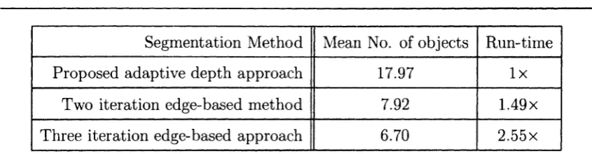
5.1 Proposed Depth Segmentation Evaluation 48
5.1.1 Performance Comparison 48 5.1.2 Operational Efficiency 48 5.2 Proposed Tracking Approach Evaluation 50
5.2.1 Handling Scale Variations in Cluttered Scenes 50 5.2.2 Handling Occlusions in Inadequate Illumination 50 5.2.3 Handling Rotation, Complex Motion and Self-Occlusion . . . . 54
5.2.4 Performance in Noisy Environments Due to the TOF Nature . 54
6 Conclusions and Future Work 58
6.1 Contributions 59 6.2 Future Work 60
CONTENTS
List of Figures
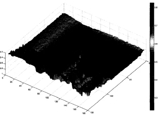
4.1 Depth and gray-scale intensity outputs of a TOF sensor 35 4.2 3D Depth map representation of the depth output obtained from a
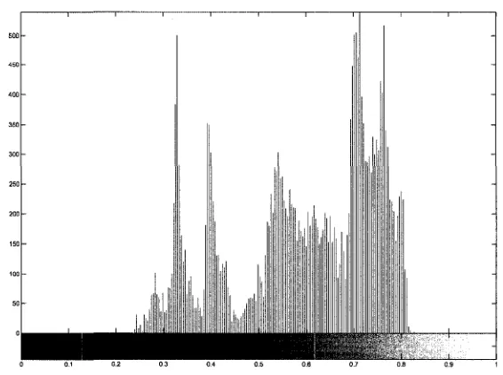
TOF sensor 35 4.3 Depth histogram presentation of a 3D scene 37
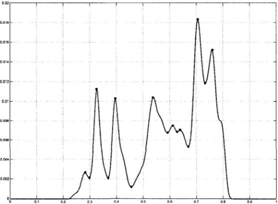
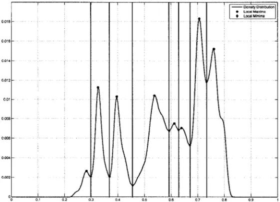
4.4 Depth density function of a depth histogram 38 4.5 Range dividers for extremum segmentation 39 4.6 Binary depth divisions resulted from the range segmentation approach 40
4.7 Object segmentation output from analysis of depth divisions 42 4.8 Objects of interest, detected from segmentation image using geometric
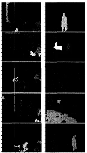
features 43 5.1 Comparison of the proposed depth-based segmentation (left) with edge
segmentation algorithms (right) 49 5.2 The proposed tracker's results for rapid scale variation in cluttered
background setting 51
5.3 Tracking results under low illumination and occlusion 52
5.4 Tracking results of multiple people under low illumination and occlusion 53 5.5 Successful tracking results under out-of-plane rotation with rapid pose
LIST OF FIGURES
5.6 Successful tracking results under self-occlusion, rapid pose change and
complex motion 56
List of Abbreviations
2D 3D CCTV CMOS CONDENSATION EKF FOV HSV i.i.d. MC pdf PF RGB SIS SMC TOF UKF Two-Dimensional Three-Dimensional Closed-Circuit TelevisionComplementary Metal-Oxide Semiconductor Conditional Density Propagation
Extended Kalman filter Field of View
Hue-Saturation-Value color space independent and identically distributed Monte Carlo
probability density function Particle Filter
Red-Green-Blue color space Sequential Importance Sampling Sequential Monte Carlo
Time of Flight
Chapter 1
Introduction
1.1 Motivation
Visual tracking is the process of detecting objects of interest from background and tracking them through consecutive frames in a video sequence. It has been one of the important topics of computer vision as it finds application in areas such as video surveillance, human-computer interaction, intelligent transportation, driver monitor-ing, pedestrian protection, medical diagnostics, and video compression.
1. INTRODUCTION
encouraging incorporation of other features to increase the tracker efficiency. In recent years, usage of depth information for object tracking is becoming popu-lar due to the availability of information about the third dimension, which provides the distances of objects from the sensor. Stereo vision systems have been prevalently exploited to determine the depth-map of the scene by means of calculating disparities from images captured from two cameras separated by a baseline. Nevertheless, the process of stereo matching to obtain depth-map information tends to be computa-tionally intense, and the results are not adequately accurate. In addition, passive stereo sensors require the presence of sufficient ambient illumination so that they can produce good quality shots. These limitations have motivated development of active depth sensors such as laser range scanners and time-of-flight (TOF) sensors [41]. TOF sensors have significant advantages over laser range scanners, which include higher accuracy, existence of vertical as well as horizontal scanning capability, pixel-level measurement quality, and considerably smaller weight and size [51].
Visual tracking can be further classified into low-level and high-level approaches. In a low-level approach, an image is segmented or classified in order to localize the blob or object without any initial hypothesis. The high-level approach, on the other hand, performs object association from one frame to the next, by generating an object hypothesis and then evaluating the likelihood of a set of given hypotheses for each frame, based on the most recent measurement. The particle filter [25, 27, 9] is one of the most successful object tracking methods that solves nonlinear cases in which noise may be non-additive and non-Gaussian, by representing simultaneous alternative hypotheses. The particle filter has been adopted as a recursive Bayesian filter in many research works such as [1, 11, 29, 39]. Besides, it has been shown to produce superior results as compared to mean shift, Kalman filter and the extended Kalman filter [1, 39].
1. INTRODUCTION
sensor, combining the high-level approach of particle filtering with a proposed bottom-up technique for object segmentation in depth images. One of the main applications of this research is in intelligent transportation systems, where the 3D profile of the driver and passengers are tracked to accomplish certain tasks. The corresponding environment consists of cluttered backgrounds, involving object occlusions and with possibly inadequate illumination settings or drastic lighting changes.
1.2 Thesis Organization
Following this chapter, chapter 2 presents a brief review of the literature in 2D and 3D visual tracking. Furthermore, the state of the art time-of-flight sensing technology for capturing 3D scene structure is described. This is followed by a review of the tracking approaches that exploit 3D sensors for acquiring input video sequences.
Chapter 3 describes the fundamentals of nonlinear Bayesian tracking and current approaches including the particle filtering method. It also presents a review of the significant research contributions in the area of particle filter tracking.
Chapter 4 is devoted to the elaboration of the developed probabilistic 3D tracking which is mainly based on adaptive depth segmentation of TOF range images. It is shown that depth histograms can be leveraged to derive a range segmentation ap-proach, in order to be applied in object detection. In addition, the developed method is exploited to define parameters of the particle filter, which is used to associate and track objects throughout the video sequence.
Chapter 5 covers experimental results of both the adaptive depth segmentation and the probabilistic tracking presented in chapter 4.
Chapter 2
Visual Tracking Literature
2.1 Overview
In visual tracking, there are three main factors that need to be considered in order to design an object tracking system. First, a suitable representation of the object should be defined. Another important step is to choose the appropriate input image features, and finally a strategy for detection of objects needs to be selected [53].
2. VISUAL TRACKING LITERATURE
as human body parts [53]. Also, object appearances can be represented using prob-ability densities, which can be either parametric (Gaussian, mixture of Gaussians) or nonparametric (Parzen windows, histograms) [53]. Template representation is an-other approach that is most suitable for tracking objects whose poses do not change noticeably during tracking. One of the advantages of templates is that they convey both spatial and appearance information, but from a single view. There also exist other appearance representations including active models and multi-view models.
Common visual features that are used in tracking are color, edge, optical flow, and texture information [53]:
• Color: The color of an object is mainly affected by the environmental illumina-tion as well as the reflectance properties of the object. Different color spaces are used for color representation in tracking, such as RGB, HSV, L*U*V, L*a*b, etc. Color is one of the most popular features used for tracking in the litera-ture. However, color is sensitive to illumination variations, hence encouraging the incorporation of other features to increase the efficiency of the tracker. • Edges: Edge information generally convey drastic intensity variations in an
image, extracted using edge detection techniques. One of its significant proper-ties is that edges are less sensitive to illumination variations compared to color features.
• Optical Flow: Optical flow is a dense field of displacement vectors which defines the translation of each pixel in a region. It is computed using the brightness constraint, which assumes brightness constancy of corresponding pixels in con-secutive frames. Optical flow is commonly used as a feature in motion-based segmentation and tracking applications.
2. VISUAL TRACKING LITERATURE
step to generate descriptors compared to color. Also, texture features are less sensitive to illumination changes than color.
Each tracking algorithm is composed of an object detection module. Object de-tection is performed either once the object appears in the scene or in every frame, considering the temporal information of consecutive frames to increase the detection efficiency. Common object detection methods include point detection, segmentation, background modeling, and supervised classifiers [53].
2.2 Segmentation
Segmentation subdivides an image into its constituent regions or objects [24]. The level to which this subdivision is carried out depends on the problem being solved. In other words, the segmentation task should end when the objects of interest have been isolated. An optimal depth segmentation algorithm should partition an image into more meaningful and easier to analyze regions with no overlap, where the final depth scene is generated by arranging all these regions together. Furthermore, segmentation methods in tracking applications should consume the least amount of processing time, as well as incur the fewest possible computational operations, due to the real-time requirement in tracking approaches. On the other hand, increasing the time efficiency should not hinder achieving acceptable results. There are two main factors to be considered in order to evaluate the performance (speed) of segmentation algorithms, i.e. number of iterations, and computational complexity.
2. VISUAL TRACKING LITERATURE
region splitting and merging.
Edge detection has been one of the popular segmentation algorithms for years. Edge-based segmentation techniques apply edge detection to extract discontinuities in the scene and segment the image [20]. In order to segment the image correctly, the identified edges should form closed boundaries. However, the resulting edge maps are often disconnected. Hence, additional processing should be performed on edge boundaries to connect isolated edges if they are within a distance-threshold from each other. Another main drawback of edge-based range segmentation algorithms is that discontinuities are smooth and hard to locate for curved surfaces in depth images, resulting in under-segmentation of range images. Thus, it is essential to inspect each of the edge-separated regions iteratively to assure that no object of interest is missed. As a result, edge detection segmentation methods are computationally intense and therefore have limited applications in real-time vision systems.
Thresholding is another popular approach for segmentation especially in applica-tions where speed is important, mainly because of its simplicity of implementation and intuitive properties. For instance, in a gray-level histogram of an image com-posed of light objects on a dark background, the objects can be separated from the background using a threshold level determined from the histogram. In this case, seg-mentation is carried out by scanning the image pixel by pixel and labeling each pixel as object or background, depending on whether the gray level of that pixel is greater or less than the threshold value. In general cases where there are three or more modes characterizing the image histogram, multilevel thresholding can be used to classify
each object [24]. Note t h a t the success of thresholding depends entirely on how well
the histogram can be partitioned.
2. VISUAL TRACKING LITERATURE
that have properties (e.g. color ranges) similar to the seed [2]. Generally, there can be one or more starting points based on the application. In cases where a priori information is not available, the same set of properties that will be used to assign pixels to regions during the growing process is calculated at each pixel. Based on the results of these calculations which form clusters, pixels close to the cluster centroids can be used as seeds. The selection of similarity criteria is crucial in the success of region growing and it depends on both the problem type and the type of image data available. Another issue in this technique is the determination of a stopping rule. As a rule, growing a region should stop when no more pixels satisfy the criteria for inclusion in that region.
Object tracking based on region growing in range images has been considered in [36], which mainly relies on road modeling. Here, a distance map is first calculated, and a region growing segmentation is performed within simulated and uncluttered traffic scenes. In [33], a depth-based tracking system in traffic scenes is described, where the employed segmentation method is based on a region growing scheme in-troduced in [36]. In order to achieve reliable results, it is necessary to apply some constraints regarding the identification of the ground surface. The background and foreground range images have to be predefined in this method, which is not suitable for real-time depth traffic environments where the camera is non-stationary. Fur-thermore, an additional preprocessing step is required to remove edges from objects using an edge detection technique. As discussed earlier, incorporating edge detection modules reduces the segmentation speed drastically, without even considering the
usage of the computationally intense region growing algorithm. Depth and intensity
2. VISUAL TRACKING LITERATURE
relying on intensity values requires the use of edge detection, not to mention the vulnerability to illumination variations. In addition, the distance map calculation is carried out in order to locate object boundaries in the scene. One necessary prepro-cessing step in this method is to eliminate out-of-range background clutter — which is done manually in each scenario, hence restricting its application.
2.3 Kernel Density Estimation
Kernel density estimation is a broadly applied technique in statistics and pattern recognition (also known as Parzen window method) [47, 19]. A kernel density esti-mate is a continuous function derived from discrete data [35]. To accurately determine the mode locations of a random variable x, which are the local maxima of its proba-bility density function p{x), a continuous estimate of the underlying density p(x) has to be defined. However, since only the discrete values of x are available, the data is convolved with a symmetric kernel function by placing a kernel in each point. There-fore, the density estimate in a given location is the average of the contributions from each kernel. However, due to the finite nature of the kernel support, only some of the points contribute to the density estimate. Let Xi, i — 1 , . . . , n, be scalar measurements drawn from an arbitrary probability distribution p(x). The kernel density estimate p(x) of this distribution is achieved using a kernel function K(u) and a bandwidth h
i—l x '
The most significant properties of kernel functions are that they should be sym-metric with bounded support and satisfy the following:
K{u) = 0 |w| > 1
J~1 V ; (2.2)
K{u) = K(-u) > 0
2. VISUAL TRACKING LITERATURE
The above formulation can be further expanded by replacing the kernel bandwidth h with a symmetric, positive definite bandwidth matrix H to include multivariate measurements.
2.4 Time-of-Flight Sensors
Time-of-flight (TOF) depth sensors are non-contact optical measurement devices that are able to acquire the entire depth image of a scene in real-time. Depth informa-tion is delivered by the solid-state sensor without any need for external circuitry. They consist of a modulated light source such as infrared, a CMOS imaging sensor consisting of an array of pixels, as well as an optical focusing system [40, 41].
Overall, TOF sensors have significant advantages over laser range scanners, in-cluding higher accuracy, existence of vertical as well as horizontal scanning, pixel-level measurement quality, and considerably smaller weight and size. A comparison of TOF sensors and laser range scanners can be found in [51].
2.4.1 T O F Principle
TOF systems operate based on the TOF principle [32]. An intensity modulated wave is synchronously emitted through the light source, propagating from the TOF sensor to the scene and is reflected by the scene back to the sensor where the sensor captures its time of flight. The phase delay between the two signals is used to determine the object's distance from the sensor. The signal phase is detected by synchronously demodulating the incoming modulated light within the detector. Let s(t) and g(t) be the incoming optical signal (with amplitude A and phase ip) and the demodulation signal, respectively.
2. VISUAL TRACKING LITERATURE
The cross correlation between the demodulation signal and the incoming signal is computed as:
1 f+%
C{T) = s(t) <g> g(t) = UrriT^ocj; / T s(t) • g(t + r)dt (2.5)
Evaluating (2.5) for phase delays of r0 = 0°, n = 90°, r2 = 180°, and r3 = 270°, the
phase ip, the offset B, and the amplitude A of the incoming signal are determined as follows.
<p = arctan (°^\ ' °^\) (2.6)
Vc(r0) - C(T2) J
B = C(To )+ C(rl )+ C(r2 ) +C(r3 ) /2 7x
^ = _V _ ( 2.8)
The object's distance from the sensor d is thus determined from tp in
d=l£ (2.9)
where,
represents the non-ambiguity distance range, /m the modulation frequency, and c the
speed of light [40].
2.5 T O F Literature
2. VISUAL TRACKING LITERATURE
2.5.1 T O F Application in Head Tracking
In [23], a head-tracking algorithm using a time-of-flight depth sensor is described, where the depth sensor is exploited to segment the background and foreground. A depth signature is determined for each segmented foreground, followed by a compari-son with depth signatures collected in training. K-means algorithm is used to cluster the training data to account for all possible cases. A correlation-based method al-locates weights to the most possible head locations, and the final head location is determined by weighted-interpolating among these locations. Although it reported promising results, this work only addresses the tracking problem for one person sit-ting in front of the camera. Furthermore, only partial self occlusion between the object's head and hand is considered and the inter-object occlusion or occlusion by the background structure are not studied. The training session is required to obtain a good model for the head location, where the head location is chosen manually.
Another head tracking algorithm using model fitting of the head's 3D depth map as an ellipse and shape matching is presented in [37]. The ellipse properties, i.e., position and size are constantly updated by a local search. Edge detection is applied on depth maps to provide depth discontinuities, followed by a Chamfer distance-based ellipse detection. The initialization of head position is not addressed in their paper and reader is referred to [44, 42]. The reason to use distance transform instead of the edge image is that the similarity measure becomes a smooth function of the shape model parameters and matching location, also allowing some degree of dissimilarity.
2.5.2 T O F Application in Visual Surveillance
2. VISUAL TRACKING LITERATURE
interest. This method can be used in non-stationary camera situations since it is not dependent upon background subtraction. The reported depth resolution for a 2.5 m range is 1 cm. The out-of-range background clutters are eliminated by manually setting a maximum acceptable distance, which is a constraint on its application. Region segmentation is performed based on a split-and-merge algorithm. Basically, foreground areas are split into smaller regions by separating their depth values into predefined depth layers (8 to 32) depending on each application. In this method, regions are grouped into sub-areas based on connected component analysis. Later on, sub-areas from different layers are merged with each other if the connections between them are regular and their layers are continuous. Next, a geometric representation is used to fit ellipses into the detected silhouette. Finally, tracking is performed by a simple method of identifying similar ellipses in the next frame. This method will achieve good results only if the relative movements are small and occlusions are rare. Also, the size of ellipsoidal model will vary for different object poses, causing inefficient results. Above all, this method depends much on the particular scene that is under investigation since it is dependent on manual selection of a depth threshold for foreground detection.
In [38], a method is presented for illumination-invariant tracking (head, hand, and body) in indoor cluttered environments using depth edges from a depth sensor. It mainly focuses on tracking the object as a whole, instead of using features for tracking. The operational domain is limited such that the target holds a distinct depth difference with respect to its surrounding environment. This technique uses potential fields, where the target is modeled as an attractor and each point outside the target is assigned a value based on its distance from the target. This task is carried out using depth image edges, based on distance transform and contour tracking.
2. VISUAL TRACKING LITERATURE
major issues such as occlusions and quick variations in body pose and appearance effectively. However, stereo systems degrade in performance in situations where there are untextured scenes because of homogeneous objects or poor lighting condition. The solution presented in this paper is to use TOF sensors that can operate under severe low-lighting conditions. Several geometrical constraints and invariants have been considered in order to simplify tracking. A simple background subtraction al-gorithm based on a pixel-wise parametric statistical model is applied to construct the background model. This model is not maintained over time once constructed, since the camera and background are assumed to be stationary. A plan-view map is also built using the intrinsic and extrinsic parameters of the camera considering the orthographic projection of the scene. This requires camera calibration which is done offline in the training stage. Tracking is performed over connected components in the blob level using a limited set of geometric features. This paper handles occlusion using Kalman filter which produces efficient results in linear situations. Based on the plan-view setup assumptions people cannot overlap each other and also should enter the scene separately.
2.5.3 T O F Application in Traffic Environment
A 3D multiple object tracking in traffic scenarios is investigated in [33]. The authors use a TOF range sensor mounted on a vehicle to acquire depth images. At first, several preprocessing filters are applied to eliminate noisy pixels from the image, as follows:
• Analysis of an amplitude minimum filter, which requires sorting all the ampli-tude values on the image and choosing an adaptive threshold to reject those pixels with low amplitude values as noise.
2. VISUAL TRACKING LITERATURE
image as well as a background range image to reject pixels with values outside the range of these two images.
• Edge pixel removal, which removes the edge pixels between objects as a neces-sary step before region growing.
The traditional region growing is exploited on the range image to segment regions of different objects. This is followed by a detailed region post-processing to deal with the problem of object over-segmentation caused by region growing. Next, the segmented objects in the current frame are associated with the objects in the previ-ous frame. An object association strategy is proposed to deal with object tracking robustly in case of merging and splitting. A Kalman filter model is constructed in the last step to correct the object positions in the current frame and predict their positions in the next frame. These predictions will be used in the next iteration for the corresponding object association.
2.6 T O F Applications in Other Areas
Except for tracking, TOF sensors have been used in other research areas such as face detection, 3D pose estimation, human computer interaction, etc.
2.6.1 Face Detection
2. VISUAL TRACKING LITERATURE
2.6.2 3D Pose Estimation
In [55], the authors present a 3D head pose estimation technique using both gray and depth information from a TOF range sensor. Depth information is used for successful head segmentation even in a cluttered scene, where a sparse optical flow is exploited at head region to estimate the 3D head motion.
Also in the paper by Fujimura et al. [22], the authors present a 3D head pose estimation approach from a sequence of images taken by a single TOF camera. They partition the human body into a number of clusters and use machine learning tech-niques for pose extraction.
2.6.3 Human Computer Interaction
In [18], a virtual keyboard system consisting of a pattern projector and a TOF range sensor is presented. The depth information from the TOF sensor is used to detect the hand region with respect to a reference frame. Furthermore, the feature models of the depth curve is analyzed to determine the exact key that was pressed.
2.7 Stereo Vision Methods
In addition to TOF systems, passive sensors such as stereo vision cameras have been used for retrieving depth information for many years. They are less expensive than active sensors, but rely on 2D information in order to calculate the range values in the scene. Therefore, their performance is degraded in low illumination environments.
2.7.1 Integrated Stereo Visual Tracking
2. VISUAL TRACKING LITERATURE
used to localize users from other objects in the background. Also, skin classification detects body parts within the isolated user silhouette, and face detection localizes the faces within those identified body parts. Each method alone can track a user under optimal conditions, but each has substantial failure modes in unconstrained environments. They find that these failures are often independent, thus by combin-ing them one can achieve relatively robust results. Head-size objects can cause false positives in the depth module, skin-colored objects can cause false positives in the color module, and face pattern detectors typically are slower and cause false positives in non-canonical poses or expressions. It is also mentioned that a key strength of this system is the use of depth estimation hardware. Tracking is performed on three differ-ent time-scales: short-term, i.e. frame to frame changes, medium-term for temporary occlusions or absences for a few minutes, and long term for absences of hours or more. In short-term tracking, region correspondences based on region position and size are considered. Here, a statistical model of multi-modal appearance is considered to re-solve correspondences between tracked users over time. The incorporated features are body shape, face appearance location, color of hair, skin, and clothes determined at each time-step. Also, mean and covariance of the represented features are used to identify users on their return to the scene. In medium term tracking, lighting con-stancy and stable clothing color are assumed, as opposed to long-term tracking, where these criteria are neglected. In the dense domain, raw range signals are smoothed to reduce the effect of low confidence stereo disparities, using a morphological clos-ing operator. A gradient operator is applied on the image, thresholded at a critical
value based on the maximum expected depth discontinuity in the depth profile of one
2. VISUAL TRACKING LITERATURE
at each frame using position and size constancy through comparison of the centroid and size of each new depth region with those of the previous frame. In other words, for each new region, the closest old region within a minimum threshold is marked as the correspondence match. In the range module and for long-term tracking, height of the user is estimated and used as an attribute of identity. In the color module, the average color of skin and hair regions, as well as an optional color histogram of clothing are considered for identification. Although stereo is used in this paper, it mainly relies on intensity features rather than depth information.
2.7.2 Head Detection Using Stereo
2. VISUAL TRACKING LITERATURE
2.8 Active Triangulation Methods
Active sensors have been exploited in [34] to present a head tracking algorithm using 3D data. A 3D sensor composed of a closed-circuit TV (CCTV) color camera and a standard slide projector is employed to acquire 3D data as well as color information. This method is based on the active triangulation principle, where color-encoded light pattern is projected onto the scene, and its deformation on the object surfaces is mea-sured. The authors use an appearance-based 3D pose detection in a Bayesian tracking framework. Depth information is used to separate body from the background, while segmentation of the head from body relies on statistical modeling of the head-torso points in 3D space. However, their approach assumes only one person in the scene. As a result, the background separation technique will encounter difficulty when applied to a complicated setting with more than one person.
2.9 Summary
In this chapter, the key components of 2D and 3D visual tracking systems have been presented. Furthermore, TOF sensors and their applications have been discussed, followed by literature review of stereo vision and triangulation tracking methods. The TOF sensor has been chosen for this research due to its advantages over other 3D sensors, one of which is its ability to provide 3D depth profiles without further processing.
Chapter 3
Nonlinear Bayesian Tracking
Tracking is one of the problems that require estimation of the state of a system using noisy measurements. l In this regard, the state-space approach is used to
model discrete-time dynamic systems. In order to analyze a dynamic system, two models should be known: The system model, describing the evolution of the state with time, and the measurement model describing the relation between the noisy measurements and the state. In the Bayesian approach to dynamic state estimation, one can construct the posterior probability density function (pdf) of the state based on all available information, including the set of received measurements. In principle, this pdf is the complete solution to the estimation problem since it includes all available statistical information. Thus, an optimal estimate of the state may be obtained from the pdf. However, for many problems an estimate is required at each time-step when a measurement is received, which leads to a recursive filter solution. In a recursive filtering approach, received data can be processed sequentially rather than as a batch
3. NONLINEAR BAYESIAN TRACKING
so that it is not necessary to store the complete data set nor to reprocess existing data if a new measurement becomes available [3]. A recursive filter consists of two main stages: prediction and update. The prediction stage uses the system model to predict the state pdf from one time-step to the next. Prediction generally translates, deforms, and spreads the state pdf, since the state is subject to unknown disturbances modeled as random noise. The update step uses the latest measurement to modify the prediction using the Bayes theorem. In the problem of tracking, the target is characterized by the state sequence {xt,t € IN}, assuming IN as the set of natural
numbers. The evolution of the state sequence is determined by the system model:
xt = ft(xt-i,vt-i) (3.1)
where ft is in general a nonlinear function of the state xt~i, and {vt-\, t e IN} is an
i.i.d. process noise sequence. The objective of tracking is to recursively estimate xt
from measurements
zt = ht(xt,nt) (3.2)
where ht is in general a nonlinear function, {nt,t € IN} is an i.i.d. process noise
sequence. In other words, we are interested in filtered estimates of xt based on the
set of all available measurements z\:t = {zi,i = 1 , . . . , t} up to time t. Therefore, it
is necessary to have the pdf p(xt\zi:t). The initial pdf p(xo\zo) = P(XQ) of the state
vector, prior, is assumed to be known. Then, in principle, the pdf p(xt\zi.,t) may be
obtained recursively in two stages: prediction and update. In the prediction stage, the system model (3.1) is utilized to obtain the prior pdf of the state at time t using the following equation, knowing that the pdf p{xt-\\z\.t-x) at time f — 1 is available.
p(xt\z1:i-i) = I p(xt\xt-i)p(xt-i\zi:t-i)dxt-i (3.3)
3. NONLINEAR BAYESIAN TRACKING
oivt-i- In the update stage and at time-step t, the measurement zt becomes available,
and this is used to update the prior using Bayes' rule
=
P^MPM^)
(3 4)where the normalizing constant
p(zt\zi:t-i) = / p(zt\xt)p(xt\zilt-i)dxt (3.5)
depends on the likelihood function p(zt\xt) defined by the measurement model and
the known statistics of n*. Note that in the update stage (3.4), the measurement zt
is used to modify the prior density to obtain the required posterior density of the current state.
The optimal Bayesian solution is based on the recursive equations (3.3) and (3.4). However, this recursive propagation of the posterior density cannot be determined analytically. Instead, there are analytical recursive solutions, i.e., the Kalman filter. Furthermore, in cases where an analytical solution is not present, extended Kalman filters and particle filters are the popular solutions that approximate the optimal Bayesian solution.
3.1 Kalman Filter
The posterior density in the Kalman filter is assumed to be Gaussian and parametrized by a mean and covariance. If p(xt-\\z\.t-\) is Gaussian it can be shown that p{xt\z\:t)
is also Gaussian with the following assumptions:
• vt-\ and nt are drawn from Gaussian distributions of known parameters.
• ft{xt-i,vt-x) is a known linear function of xt-\ and vt-\.
3. NONLINEAR BAYESIAN TRACKING
As a result, the system and measurement models, (3.1) and (3.2), become as follows:
xt = Ftxt-\ +vt-i (3.6)
zt = Htxt + nt (3.7)
Ft and Ht are known matrices defining the linear functions. The covariances of vt-\
and nt, which are assumed to be of zero-mean and statistically independent, are Qt-i
and Rt, respectively. Note that the system and measurement matrices as well as noise parameters can be time variant.
The Kalman filter, derived from (3.3) and (3.4), can be expressed as the following recursive equations:
p{xt-\\z\*-\) =J\f(xt-i;mt-i\t-i;Pt-i\t-i) (3-8)
p(xt\zi..t-i)=M(xt;mt\t-i;Pt\t-i) (3.9)
p(xt\zi:t) = M (xt; mm; Pt\t) (3.10)
where
mt\t-i = Ftmt-i\t-i (3.11)
Pt\t-i = Qt-i + FtPt^t_xF? (3.12)
mt\t = mt\t-i + Kt(zt - Htmt\t-i) (3.13)
Pt\t = Pt\t-i ~ KtHtPt\t-i (3.14)
and where M(x; m, P) is a Gaussian density with argument x, mean m, and covariance P. Moreover,
St = HtPt^H? + Rt (3.15)
Kt^Pn-iHfSr1 (3.16)
are the covariance of the innovation term zt — Htmt\t^i, and the Kalman gain,
3. NONLINEAR BAYESIAN TRACKING
The above is the optimal solution to the tracking problem as long as the highly restrictive assumptions hold. According to literature, the Kalman filter provides the best result in a linear Gaussian environment.
3.2 Extended Kalman Filter
The above assumptions do not hold in most cases, and as a result, the Kalman filter cannot be exploited. In general, the system and measurement models, (3.1) and (3.2), are nonlinear and thus cannot be written as (3.6) and (3.7). The Extended Kalman Filter (EKF) approximates nonlinearity by local linearization of these functions. In this algorithm, p(xt\zi-t) is approximated by a Gaussian
p(xt-i\zi-.t-i) ~ Ar(a;t_i;mt-i|t-i;i't-i|t-i) (3.17)
p(xt\zi-.t-i) ~ M (a;t; mtit-x; Pt\t-i) (3.18)
P(xt\zv.t) ^M(xt;mtlt;Ptlt) (3.19)
where,
mt\t-i = ft(mt-i\t-i) (3.20) Pt\t-i = Qt-i + FtPt^t^F? (3.21)
mt\t = mt\t-i + Kt (zt - ht(mt\t-i)) (3-22)
Pt\t - Ptlt-i - KtHtPt\t-i (3.23)
and where ft(-) and ht(-) are nonlinear functions, and Ft and Ht are local linearization
of these nonlinear functions:
P dft{x)
dx
H = dht^
dx
(3.24) x = mt_1it_1
3. NONLINEAR BAYESIAN TRACKING
St = HtPt^H? + Rt (3.26)
Kt = Pt\t^HjS-tx (3.27)
The EKF achieves linearization using the first term of the Taylor series expansion of the nonlinear function. A higher order EKF that considers further terms of the Taylor series has been achieved, but its intensive complexity has prevented it from being widely used.
3.3 Unscented Kalman Filter
Some researchers have proposed the use of the unscented transform in EKF, which yields the unscented Kalman filter (UKF) [30, 49, 50]. UKF considers a set of points that are deterministically selected from the Gaussian approximation to p(xt\z\-_t).
These points are all propagated through the nonlinearity, and the parameters of the Gaussian approximation are re-estimated. This filter has been shown to outperform EKF in some problems, mainly because of its better approximation of nonlinearity.
Nevertheless, the EKF and UKF both approximate p(xt\zi[t) to be Gaussian. If
the true density is non-Gaussian (i.e., bimodal), then a Gaussian will never be able to represent it satisfactorily, in which case, the particle filter will produce better results compared to EKF and UKF [4].
3.4 Particle Filter
3. NONLINEAR BAYESIAN TRACKING
density is represented by a set of random samples with associated weights, which are used to compute estimates. As the number of samples becomes very large, this MC approximation becomes an equivalent representation to the usual functional descrip-tion of the posterior pdf, and the particle filter approaches the optimal Bayesian estimate.
Let {^ot'^tli^i denote a random measure that approximates the posterior pdf p(%0:t\zi:t)> where {XQ.V i = 0 , . . . , Ns} is a set of support points with associated weights
{wlt, i = 1 , . . . , iVs} and Xo-t = {xj,j = 0 , . . . , t} is the set of all states up to time t.
The weights are normalized such that £V wt = 1 • Then, the posterior density at t
can be approximated as
p(x0:t\z1:t) » ^T w%t8(x0..t - x%0.t) (3.28)
which is a discrete weighted approximation to the true posterior, p(x0:t\zi:t)- The
weights are chosen using the principle of importance sampling [5, 17]:
Let p(x) oc 7r(x) denote a probability density function from which it is difficult to draw samples but for which n(x) can be evaluated (as well as p(x) up to propor-tionality). Let x1 ~ q(x),i = 1,...,NS be samples that are easily generated from
a proposal q(-) called importance density. Then, a weighted approximation to the density p(-) is given by:
Ns
p(x)^Yjwi6(x-'xi) (3-29)
where
w* oc ^ 1 (3.30)
is the normalized weight of the i-th particle. As a result, considering the samples xl0:t
being drawn from the importance density q{xo-t\zi.t), the weights in (3.28) are defined
by (3.30) to be
3. NONLINEAR BAYESIAN TRACKING
At each iteration of the sequential case, an approximation to p(xo-.t-i\zi:t-i) is
available, and it is desirable to approximate p(xQ[t\zi:t) with a new set of samples. If
the importance density is chosen such that
q{xo-.t\zi:t) =q(xo-.t-i\zi:t)q(xo..t-i\zi..t-i) (3.32) then samples xl0.t ~ q(x0:t\z1:t) can be obtained by augmenting each of the existing
samples xl0.t_x ~ q(xo:t-\\z\-.t-\) with the new state x\ ~ q(xt\xo:t-i,Zi..t). To
ob-tain the weight update equation, p{xQ-t\zi-t) is expressed in terms of p(a;o:t-i|2i:t-i),
p{zt\xt), andp(a;t|a;t_i).
P(zt\x0:t\zi;t-i)p{x0:t\z1:t-i)
P(x0:t\zi;t)
V\Zt\Z\;t-\)
n(y.AT.n Ay-, . 1 \r>( r. I T ^ , i I 7-, , -,
-p(x0:t-i\zi:t-i) (3.33)
p(Zt\Zl:t-l)
p(zt\x0:t\zi.t-i)p(xt\xo.i-l\zl..t-i)
P{Zt\Zi:t-l)
p(zt\xt)p(xt\xt-i) . , .
= _ - p{XM-x\Z\:t-\)
p{zt\zv.t-\)
p(xo-.tW:i) (xp{zt\xt)p(xt\xt-i)p{xQ..t-i\zi;t-i) (3.34)
The weight update equation can be derived by substituting (3.32) and (3.34) into (3.31):
• p(ztNM^k-lM4:t-lk:t-l)
yj (x .—_ . _ — . . _
q{AWo-.t-i,Zv.t)q{xl:t_1\z1,t-.i)
i P{zt\x^p{x\\x\_l) _ Wt_i i. i r
-q\Xt\XQ:t-\i Z^t)
In the common case when only a filtered estimate of p{xt\z\.t) is required at
each time-step, the importance density becomes only dependent on xt-i and zt, i.e.,
q(xt\xo:t-i, z1:t) = q(xt\xt-i,Zt). Therefore, only x\ need to be stored and the history
of the states (a^t-i) a nd observations {zvt_x) is disregarded. The weight in this case
becomes
i , piztlxppixWxU)
w
'"
w" M^,*)
(3"
36)Finally, the posterior filtered density p(xt\zi:t) can be approximated as
3. NONLINEAR BAYESIAN TRACKING
It can be shown that as Na —• oo, this approximation approaches the true posterior
density p{xt\zv.t)- The particle filter consists of recursive propagation of the weights
and support points as each measurement is received sequentially.
3.5 Particle Filter in Tracking
In the high-level approach to tracking, objects are associated between consecutive frames by generating a set of object hypotheses, followed by evaluation of the cor-responding likelihood for each frame based on the most recent measurement. The particle filter is able to represent multiple hypotheses simultaneously. In addition, it is one of the most efficient object tracking methods in nonlinear situations that involve non-additive and non-Gaussian noise.
3.5.1 CONDENSATION
CONDENSATION algorithm [27] uses "factored sampling", in which the probability distribution of possible interpretations is represented by a randomly generated set. It exploits dynamic models (transition or prior densities) along with visual observations (measurements), to propagate the random set over time. Given the prior, and an observation density that characterizes the statistical variability of image data z given a state x, a posterior distribution can, in principle, be estimated for xt given zt at
successive times t.
Spatio-temporal tracking has been dealth thoroughly by Kalman filtering, in the relatively clutter-free case in which densities can be modeled as Gaussian. These solutions produce relatively poor results in clutter which causes the density for xt to
be multi-modal and therefore non-Gaussian.
The state of the modeled object at time t is denoted xt and its history is Xt =
3. NONLINEAR BAYESIAN TRACKING
No assumptions on linearity, Gaussian behavior or unimodal distribution are made. CONDENSATION is an iterative algorithm with each time-step a self-contained iter-ation of factored sampling. The output of an iteriter-ation at each time-step is a weighted sample set 14" > n = 1,.. .,N> with weights 717, representing approximately the conditional state density p(xt\Zt) at time t. The method begins with a prior density
at time t, which is the posterior prediction at time t — 1, i.e., p(xt\Zt-i). This prior
is derived from the output of the previous time-step, < (st-i) flt-i )> n — I,..., N>
o{p(xt-i\Zt-i). The aim is to maintain, at successive time-steps, sample sets of fixed
size N. The first step is to sample N times from the set \ s|_! >, choosing a given element with probability < 7rt_\ >. The elements with high weights may be chosen
sev-eral times in the new set, while others with relatively low weights may not be chosen at all. Next, each element in the new set undergoes the predictive steps, i.e., drift and diffusion. At this stage, the sample set < s^ !> for the new time-step has been generated with no associated weight. In the final step, the observation density p(zt\xt)
is used to generate weights, leading to the sample-set representation < (s\n , ir\; ) [
of state-density for time t.
3.5.2 ICONDENSATION
Followed by the introduction of CONDENSATION algorithm for visual tracking, a probabilistic framework, i.e. ICONDENSATION [28], was proposed to integrate the low-level and high-level tracking approaches using the statistical approach of importance sampling combined with the CONDENSATION algorithm.
3. NONLINEAR DAYESIAN TRACKING
been performed using color segmentation to detect skin-colored blobs and incorpo-rating this information with a hand contour tracker.
3.5.3 Color-based Probabilistic Tracking
The deterministic methods exploiting color histogram principle rely on the determin-istic search of a window whose color content matches a reference histogram color model. Bradski [8] uses a histogram of skin color in HSV color space to determine the likelihood of skin occurring at each pixel, using histogram back-projection to replace each pixel with the probability associated with that HSV value in the skin color his-togram. In [12] the target appearance model is a distribution of colors represented by a histogram probability qu, which is compared with a histogram of target candidate
pu observed within the current mean-shift window. The comparison is based on the
histogram similarity using the Bhattacharyya coefficient. Basically, the current frame is deterministically searched for a region, a fixed-shape variable-size window, whose color content best matches a reference color model. Starting from the final location in the previous frame, it proceeds iteratively at each frame so as to minimize a dis-tance measure to the reference color histogram. Excellent tracking results on complex scenes are demonstrated in [8, 10, 12]. This deterministic search might however run into problems when parts of the background nearby exhibit similar colors or when the tracked object is completely occluded for a while.
Perez et al. [43] have applied the SMC tracking technique on a tracker based on the color histogram distance. Incorporating the particle filter allows better handling
color c l u t t e r in t h e b a c k g r o u n d , a s well a s c o m p l e t e occlusion of t h e t r a c k e d o b j e c t s
3. NONLINEAR BAYESIAN TRACKING
studied sequence. This type of tracker is very useful for tracking objects of interest that are of any kind and show drastic spatial changes through the sequence, due to pose changes, partial occlusions, etc. It relies on the same principle of comparing color contents of candidate regions with a reference color histogram, while being embedded within a SMC framework. This requires construction of a color likelihood based on color histogram distances, coupling of this data model with a dynamical state space model, and sequential approximation of the resulting posterior distribution with a particle filter. The use of a sample-based filtering technique allows the simultaneous tracking of multiple posterior hypotheses, which is very crucial to avoid background distraction and recover after partial or complete occlusions. A second-order auto-regressive dynamics is chosen as the dynamic model of the system. The color model is obtained by histogram technique in the HSV color space [21]. Within the candidate region, a kernel density estimate of the color distribution at each time t, qt(x) =
{qt{n;x)}n_1 N, is used as the color model. This model associates a probability
to each of the N color bins. At time t, the color model qt{x) associated with a
hypothesized state x is compared to the reference color model q* = {q*(n)}n=l N,
which is normalized and constructed at an initial time t0 at a location x*o, either
manually or automatically by a detection module. The likelihood function must give importance to the candidate histograms with minimum distance to the reference histogram. The Bhattacharyya distance based on the Bhattacharyya coefficient is used to identify the closest matches.
3. NONLINEAR BAYESIAN TRACKING
priori distribution provided by the particle filter. To weigh the sample set, the Bhat-tacharyya coefficient is computed between the target histogram and the histogram of the hypotheses.
3.6 Other Methods
3.6.1 Mean Shift Embedded Particle Filter
The particle filter performs a random search guided by a stochastic motion model to obtain an estimate of the posterior distribution describing the object's configuration. On the other hand, mean shift, a typical and popular variational method, localizes an object based on minimizing a cost function. The search method of the particle filter is stochastic and model-driven, while in mean shift, it is deterministic and data-driven. In addition, the particle filter applies a recursive Bayesian filter based on propagation of sample set over time, maintaining multiple hypotheses at the same time and using a stochastic motion model to predict the position of the object. Maintaining multi-ple hypotheses allows the tracker to handle clutters in background, also recover from failure or temporary distraction. Mean shift, on the other hand, uses only one hypoth-esis, which is computationally effective but is prone to converge to local maximum. A common problem in conventional particle filters is the degeneracy phenomenon, where all but one sample will have negligible weight after a few iterations [3]. In other words, these samples may have very low likelihood and their contribution to the posterior estimation becomes insignificant, which is computationally ineffective.
track-3. NONLINEAR BAYESIAN TRACKING
ing to handle skin color variations over time due to illumination changes. In their approach, mean shift analysis is applied to each sample based on observation den-sity, after being weighted by observation. After mean shift iterations, samples are
"herded" to the local modes of the observation. Since the samples are moved to have large weights, the algorithm concentrates on samples with large weights. Therefore, the degeneracy problem is efficiently overcome. Also, if the iteration times are set properly, the resultant samples will not contain too many repeated points and the problem of impoverishment is reduced.
3.7 Summary
Chapter 4
Probabilistic 3D Tracking Based
on Adaptive Depth Segmentation
This chapter presents the problem formulation and implementation steps of the pro-posed probabilistic object tracking based on the TOF sensor data. The goal is to detect objects of interest in the scene and consecutively track them through video sequences obtained by TOF sensor.
4. PROBABILISTIC 3D TRACKING BASED ON ADAPTIVE DEPTH SEGMENTATION
(a) Depth image (b) Intensity image Figure 4.1: Depth and gray-scale intensity outputs of a TOF sensor
4. PROBABILISTIC 3D TRACKING BASED ON ADAPTIVE DEPTH SEGMENTATION
scene can have
• cluttered background • various lighting settings • and complex motion patterns.
Also, multiple people can be present in the scene, navigate, enter, and exit the tracking environment.
4.1 Adaptive Depth Segmentation
This section describes a novel approach to segment objects in cluttered 3D environ-ments using depth map distribution produced from a depth histogram of the scene. In the initial processing stage, depth images derived from the TOF sensor are passed through a noise-removing filter to remove noisy depth measurements around the ob-ject boundaries. The following processing steps are depth histogram evaluation, de-termination of the depth density function, segmentation using depth extrema, object detection and object association.
4.1.1 Depth Histogram Evaluation
4. PROBABILISTIC 3D TRACKING BASED ON ADAPTIVE DEPTH SEGMENTATION
Figure 4.3: Depth histogram presentation of a 3D scene
image is denoted by I : 5ft2 —> (a, /?) where (a, /?) is the dynamic range of the pixel
values. The discrete depth histogram of I over iV bins is defined as
K = {hzm^,2,...,N (4-1)
where, hz(i) corresponds t o the number of pixels that are located at distance i from
the camera.
4.1.2 Depth Density Function
In order t o segment depth images, it is necessary t o form the underlying
continu-ous distribution t h a t the discrete histogram measurements hz are drawn from. For
this purpose, the kernel density estimation technique is applied t o approximate this
distribution from depth histogram information t o facilitate gradient estimation and
local extrema detection. Denoting the scalar measurements Zj, i = 1,... ,N from a
4. PROBABILISTIC 3D TRACKING BASED ON ADAPTIVE DEPTH SEGMENTATION
0.5 0.6 07 0.8
Figure 4.4: Depth density function of a depth histogram a kernel function K(u) with a bandwidth A as
Z — Z;
A (4.2)
H(z) has all the properties of a pdf, and thus is called the depth density function. The resulting depth density function for the depth histogram of Fig. 4.3 is given in Fig. 4.4.
4.1.3 Range Segmentation from Extremum D a t a
In the next step, the resulting depth density function H(z) is further analyzed to derive the local maxima and minima vectors, T and 7 from equations (4.3) and (4.4), respectively. The i-th element of T over an interval [a, b] where the distribution is unimodal is expressed as:
Tj = argmaxH(z) . (4.3)
4. PROBABILISTIC 3D TRACKING BASED ON ADAPTIVE DEPTH SEGMENTATION
Figure 4.5: Range dividers for extremum segmentation Then,
7j = argmmH(z) , (4.4)
Ri = {r, < z < rj+1] (4.5)
where, j — 1, 2 , . . . , M — 1, and M is the total number of the local maxima.
Upon determination of the local extremum points of the depth density function, a set of range dividers Sk, k — 1 , . . . , M + 1, can be evaluated from (4.6). To better illustrate this process, the corresponding local extremum points as well as range dividers for Fig. 4.4 are highlighted in Fig. 4.5.
Sk=< a
fc-i
0
k=l 2<k<M
k = M + l
(4.6)
4. PROBABILISTIC 3D TRACKING BASED ON ADAPTIVE DEPTH SEGMENTATION
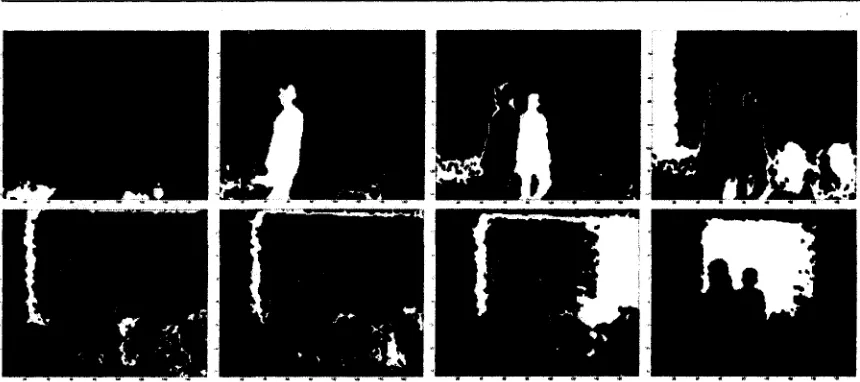
Figure 4.6: Binary depth divisions resulted from the range segmentation approach order to separate adjacent and overlapping objects, denoted by:
&i(x,y) = 1 Si < I(x, y) < Si+i
0 otherwise
(4.7)
where / = 1,2,..., M, and I is the depth image, (x, y) correspond to the horizontal and vertical pixel coordinates in the image, respectively.
In essence, each division forms a binary image containing pixels with depth values between two consecutive range dividers. A set of depth divisions achieved with this approach is demonstrated in Fig. 4.6. It is noteworthy to mention that range dividers are chosen adaptively for each image. Adaptive selection ensures that the algorithm can be applied on unconstrained environments without a priori information about the scene, including number of objects and background settings.
4.1.4 Object Detection
4. PROBABILISTIC 3D TRACKING BASED ON ADAPTIVE DEPTH SEGMENTATION
regions of isolated noises or inter-objects pixels. There exists at least one object for each division D; that is localized in that depth range.
D,
= £ a + 5 > >
(
48)
where N\ and N2 represent the total number of significant objects and insignificant regions in the corresponding depth division, respectively.
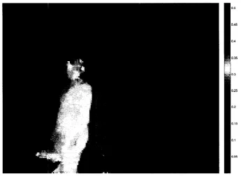
The total number of objects in the scene is determined by inspecting each divi-sion's objects, as stated above. These objects can be further classified based on their properties such as their associated mean depth in order to be exploited in the sub-sequent procedures. Also, human candidates are detected based on their geometric features, e.g., aspect ratio and relative size to depth mean. Segmentation output of this method is further illustrated in Fig. 4.7, where each object is assigned a seg-mentation label. By further analyzing the properties of segmented objects, objects of interest can be detected, as demonstrated in Fig. 4.8.
4.1.5 Object Association
To compare and match two objects from consecutive frames, it is necessary to form a similarity measure using a distance metric between their signatures. An object signature is defined by a concatenation of its X, Y, and Z histograms as
s = [hx hy hz] . (4.9)
There exist several metrics including the Euclidean distance, histogram intersec-tion, Bhattacharya distance, etc. Here, a similarity metric derived from the Bhat-tacharya coefficient is used since it has been established as an efficient metric for comparing arbitrary histogram-based distributions [13]. The distance between two discrete distributions is defined as
4. PROBABILISTIC 3D TRACKING BASED ON ADAPTIVE DEPTH SEGMENTATION
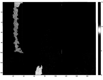
20 40 60 60 100 120 140 160
Figure 4.7: Object segmentation output from analysis of depth divisions where
N
p[hi, hj] = ] T hi(n)hj(n) (4.11)
n = l