CAO, WEIHUA. Improving Efficiency and Robustness of Doubly Robust Estimators in the Presence of Coarsened Data. (Under the direction of Dr. Marie Davidian and Dr. Anastasios A. Tsiatis).
by Weihua Cao
A dissertation submitted to the Graduate Faculty of North Carolina State University
in partial fullfillment of the requirements for the Degree of
Doctor of Philosophy
Statistics
Raleigh, North Carolina 2009
APPROVED BY:
Dr. Dennis Boos Dr. Daowen Zhang
Dr. Marie Davidian Dr. Anastasios A. Tsiatis
DEDICATION
BIOGRAPHY
ACKNOWLEDGMENTS
I owe my deepest gratitude to to my advisors, Dr. Marie Davidian and Dr. Anastasios Tsiatis. I feel so fortunate and hornored to have you as my advisors. Your encouragement, talented guidance and support are always the driving forces during my Ph.D. study. You not only help me with these specific research problems, but more importantly also show me the right way to do research, which is a vivid description of the old saying: teach a man how to fish feeds for life. I only wish I did not let you know in the past three years.
I would like to express my sincere appreciate to Dr. Dennis Boos and Dr. Daowen Zhang, for their serving on my committee, for their valuable suggestions on this research, and for their help during my job hunting. I also would like to thank their tutoring since I took five great courses from them.
It is an honor for me to be in the last class of Dr. Bibhuti Bhattacharyya before he retired. It never stopped fascinating me that how could he make measure theory so interesting and full of fun. He set a role model in teaching for me. I am thankful to Dr. Pam Arroway for her help during my graduate study. I also would like to thank my managers at GlaxoSmithKline, Dr. Mandy Bergquist and Dr. Karen Chiswell, who taught me a lot of things in industry and guided me through my one year graduate industrial trainee over there.
I am deeply indebted to my parents, brothers, wife and daughter for their endless love and support. Special thanks go to my wife Zhi and my daughter Amy, you are the meaning of my life.
TABLE OF CONTENTS
LIST OF TABLES . . . vi
1 Improving efficiency and robustness of the doubly robust estimator for a population mean with incomplete data . . . 1
1.1 Introduction . . . 1
1.2 Existing doubly robust estimators . . . 2
1.3 Alternative doubly robust estimators . . . 4
1.4 Enhanced propensity score model . . . 9
1.5 Simulation studies . . . 10
1.6 Discussion . . . 11
1.7 Details . . . 13
1.7.1 Optimal, doubly robust estimator for a treatment mean difference . . . 13
1.7.2 Enhanced propensity score and stabilized weights . . . 19
1.7.3 Calculation of asymptotic variances . . . 20
1.7.4 Asymptotic bias under local misspecification . . . 23
2 Improving Efficiency and Robustness of Doubly Robust Estimators in the Presence of Coarsened Data . . . 27
2.1 Introduction . . . 27
2.2 General coarsened data framework and coarsening at random . . . 30
2.3 Inferential objective and doubly robust estimators . . . 31
2.4 Existing and proposed doubly robust estimators . . . 33
2.5 Application to ACTG 175 . . . 39
2.6 Simulation studies . . . 42
2.7 Discussion . . . 45
2.8 Details . . . 46
2.8.1 Derivation of approximate standard errors via the sandwich method . . . . 46
2.8.2 Derivation of conditional expectations implied by assumed mixed models in Section 2.5 . . . 50
2.8.3 Derivation of conditional expectations implied by assumed mixed model in Section 2.6 . . . 52
Bibliography . . . 54
Appendices . . . 57
SAS code for Chapter 1 . . . 58
LIST OF TABLES
Table 1.1 Simulation results based on 1000 Monte Carlo replications for the Kang and Schafer scenario. Sample size is 200. Bias is Monte Carlo bias, RMSE is root mean square error, MAE is median of absolute errors, MCSD is Monte Carlo standard deviation, AveSE is average of sandwich standard errors, Cov is Monte Carlo coverage of 95% Wald confidence intervals, OR is outcome regression, and PS is propensity score. Smallest, median, second largest, and largest standard errors for entries in Table 1.1, 1.2 : BIAS,(0.04, 0.08, 0.39, 5.58); AVESE, (0.0008, 0.004, 0.58, 6.64); COV, (0.006, 0.007, 0.015, 0.015). . . 14
Table 1.2 Simulation results based on 1000 Monte Carlo replications for the Kang and Schafer scenario. Sample size is 1000. Bias is Monte Carlo bias, RMSE is root mean square error, MAE is median of absolute errors, MCSD is Monte Carlo standard deviation, AveSE is average of sandwich standard errors, Cov is Monte Carlo coverage of 95% Wald confidence intervals, OR is outcome regression, and PS is propensity score. Smallest, median, second largest, and largest standard errors for entries in Table 1.1, 1.2 : BIAS, (0.04, 0.08, 0.39, 5.58); AVESE, (0.0008, 0.004, 0.58, 6.64); COV, (0.006, 0.007, 0.015, 0.015). . . 15
Table 1.3 Simulation results based on 1000 Monte Carlo replications for the Tan scenario. Sample size is 200. Entries are as in Table 1.1. The Tan and Kang and Schafer scenarios are distributionally identical in the “OR correct, PS correct” case. Smallest, median, second largest, and largest standard errors for entries in Table 1.3, 1.4: BIAS, (0.04, 0.08, 0.76, 5.66); AVESE, (0.0008,0.004, 1.59, 9.78); COV, (0.006, 0.007, 0.010, 0.015). . . 16
Table 1.4 Simulation results based on 1000 Monte Carlo replications for the Tan scenario. Sample size is 1000. Entries are as in Table 1.1. The Tan and Kang and Schafer scenarios are distributionally identical in the “OR correct, PS correct” case. Smallest, median, second largest, and largest standard errors for entries in Table 1.3, 1.4: BIAS, (0.04, 0.08, 0.76, 5.66); AVESE, (0.0008,0.004, 1.59, 9.78); COV, (0.006, 0.007, 0.010, 0.015). . . 17
Table1 2.1, 2.2: Bias, (0.019, 0.033, 0.067, 0.077); AveSE, (0.004, 0.022, 0.086, 0.340); Cov, (0.007, 0.008, 0.010, 0.011). . . 44
Chapter 1
Improving efficiency and robustness of
the doubly robust estimator for a
population mean with incomplete data
1.1 Introduction
The challenge of estimating a population mean response on the basis of incomplete data arises in many settings. Nonresponse in sample surveys or dropout and noncompliance in clinical trials may lead to missing outcomes for some subjects; likewise, making causal inference on a treat-ment mean may be viewed as a missing data problem, where potential outcomes under treattreat-ment are “missing” for subjects actually observed to receive control (Kang and Schafer, 2007). In these situations, unless the missingness mechanism is “completely at random” (Rubin, 1976), it is well known that the naive sample mean based on the “complete cases” is a biased estimator.
If missing data can reasonably be assumed missing at random, or, equivalently, if the no unmeasured confounders assumption (Rosenbaum and Rubin, 1983; Robins, Hern´an, and
1987; Lunceford and Davidian, 2004). These methods require correct specification of the model for outcome regression or propensity score, respectively. Robins et al. (1994) identified a class of “augmented inverse probability weighted” estimators that involve modeling both the outcome regression and propensity score, with the efficient member of the class obtained when both models are correct. Scharfstein, Rotnitzky, and Robins (1999) noted that estimators in this class are “doubly robust” in that they are consistent for the true population mean even if one of the outcome regres-sion or propensity score models (but not both) is misspecified. Given the protection afforded by this property, these estimators have been advocated for routine use (Bang and Robins, 2005). However, Kang and Schafer (2007) demonstrated via simulation that the usual doubly robust estimator can be severely biased when both models are misspecified, even if they are “nearly” correct, and that bias is especially problematic when some estimated propensity scores are close to zero, yielding very large “weights.” Estimation based on an outcome regression model only performed much better under misspecification in the Kang-Schafer simulation scenario, leading the authors to warn against use of doubly robust estimators in practice. Tan (2006) discussed alternative approaches to constructing doubly robust estimators that may alleviate some of these difficulties. In this chapter, we propose doubly robust estimators that may yield improved performance relative to existing competitors.
1.2 Existing doubly robust estimators
As in Kang and Schafer (2007), we consider the standard missing data set-up; the spirit of the developments is equally relevant to the causal inference context. Considernsubjects drawn at random from a population of interest, where the ideal, “full” data are (Yi, Xi), i = 1, . . . , n, independent and identically distributed acrossi;Yiis the response or outcome; andXi is a vector of covariates. As in Section 1.1,Yiis not available for all subjects; thus, the data actually observed are independent and identically distributed(RiYi, Ri, Xi),i= 1, . . . , n, whereRi = 1or 0 asYiis observed or missing. The goal is to estimate the population mean,µ=E(Y), on the basis of these observed data. Throughout, assume responses are missing at random (Rubin, 1978) in thatYiand
Ri are conditionally independent givenXi.
(Lunceford and Davidian, 2004) that the “inverse probability weighted” estimators
b
µIP W1 =n−1 n X
i=1
RiYi
π(Xi,bγ) and µbIP W2= ( n
X
i=1
Ri
π(Xi,bγ)
)−1 n X
i=1
RiYi
π(Xi,bγ) (1.1) are consistent forµifπ(X, γ)is correctly specified; that is,π0(X) =π(X, γ0)for someγ0. This is because
E
½
RY π0(X)
¾ = E · E ½ RY
π0(X) |(Y, X) ¾¸
=E
·
E{R|(Y, X)} Y
π0(X) ¸
= E
½
E(R|X) Y
π0(X) ¾
=E(Y),
where the third equality follows the missing at random assumption. Note thatπ(X,bγ) should be greater than zero almost surely.
Alternatively, because under missing at random E{E(Y | R = 1, X)} = E{E(Y |
X)} = E(Y), lettingh0(X)denote the true outcome regressionE(Y | X), it is natural to adopt a modelh(X, ξ) forh0(X), estimateξ by someξbusing the “complete cases”{i :Ri = 1}, and estimateµby
b
µOR=n−1 n X
i=1
h(Xi,ξb), (1.2) which is consistent forµifh(X, ξ)is correctly specified; that is,h0(X) = h(X, ξ0)for some ξ0, and ifξbis consistent forξ0. Becauseξbis based only on the complete cases, if the distributions ofX conditional onR= 1andR= 0differ, (1.2) involves extrapolation.
From Robins et al. (1994) and Tsiatis and Davidian (2007), all estimators forµthat are consistent and asymptotically normal when the propensity score model is correct are asymptotically equivalent to an estimator of the form
n−1
n X
i=1 ½
RiYi
π(Xi,bγ)
+Ri−π(Xi,bγ)
π(Xi,bγ)
L(Xi) ¾
(1.3)
for arbitrary L(X). Estimators in class (1.3) are referred to as “augmented inverse probability weighted” because they have the form ofbµIP W1 in (1.1) plus an “augmentation” term depending onL(X);bµIP W1 is obtained whenL(X) ≡0. From Robins et al. (1994), the estimator with the smallest asymptotic variance among those in class (1.3) (so withπ(X, γ)correct) is
b
µDR =n−1 n X
i=1 ½
RiYi π(Xi,γb) −
Ri−π(Xi,γb)
π(Xi,bγ) h(Xi, b
ξ) ¾
takingL(Xi) =−h(Xi,ξb), whereh(X, ξ)is correctly specified, andξbis consistent forξ0. Scharf-stein et al. (1999) noted thatµbDR remains consistent if only one of the outcome regression model
h(X, ξ)or the propensity score modelπ(X, γ)is correctly specified, but is inconsistent if both are misspecified; this property is referred to as “double robustness.” Ifh(X, ξ)is correct, thenµbORis at least as efficient asµbDR(Tan, 2007) but is inconsistent otherwise, while double robustness of (1.4) affords protection against such misspecification.
The estimator (1.4), withγestimated by maximum likelihood andξestimated by ordinary or iteratively reweighted least squares is generally regarded as the “usual” doubly robust estimator. Kang and Schafer (2007) and Tan (2006) identified alternative doubly robust estimators, all involv-ing models for the propensity score and outcome regression and some appearinvolv-ing to have forms outside the “augmented” class (1.3). The former authors attributed poor performance of (1.4) when the propensity or both models are misspecified in part to “inverse weighting” by the propensity score. Tsiatis and Davidian (2007) noted that such alternative estimators can be rewritten in the form (1.3) and used semiparametric theory to argue that poor performance when one or the other model is incorrect may be partly a consequence of the method used to estimateξ. In Section 1.3, we identify doubly robust estimators from this perspective. When both models are correct andγis esti-mated by maximum likelihood, all doubly robust estimators are consistent with the same asymptotic variance; moreover, the asymptotic properties do not depend the method used to estimateξ (Tan, 2007; Tsiatis and Davidian, 2007).
1.3 Alternative doubly robust estimators
In this section, we focus on estimation ofξin a posited outcome regression modelh(X, ξ), possibly nonlinear inξ, to identify doubly robust estimators with desirable properties. To fix ideas, we consider first a fully specified propensity score modelπ(X), say, involving no unknown param-eters; we relax this shortly. Suppose, for some estimatorξbforξ, we estimateµby
n−1
n X
i=1 ½
RiYi π(Xi) −
Ri−π(Xi)
π(Xi) h(Xi, b
ξ) ¾
. (1.5)
We now examine how to estimateξ to achieve the estimator forµof form (1.5) that is (i) doubly robust and, (ii) if the propensity score is correctly specified, has smallest asymptotic variance among all estimators forµof form (1.5) usingh(X, ξ), even ifh(X, ξ)is incorrect.
may not be correctly specified. It is straightforward to show that using any estimatorξbin (1.5) leads to a consistent estimator forµwhose asymptotic variance is the same as that of
n−1
n X
i=1 ½
RiYi
π0(Xi) −
Ri−π0(Xi)
π0(Xi) h(Xi, ξ
∗)
¾
, (1.6)
whereξ∗is the limit in probability ofξb. Using var(·) =E{var(· |X, Y)}+var{E(· |X, Y)}, this variance is proportional to
var ½
RY π0(X) −
R−π0(X)
π0(X) h(X, ξ
∗)
¾ =E
·
1−π0(X)
π0(X) {Y −h(X, ξ
∗)}2 ¸
+var(Y). (1.7)
A natural objective is to identify the value of ξ∗ (and corresponding estimators ξbconverging in probability to it) such that (1.7) is minimized whether or noth(X, ξ)is correct. Lettinghξ(X, ξ) =
∂/∂ξ{h(X, ξ)}, note that (1.7) is minimized by choosingξ∗as the solution to
E[{1−π0(X)}π0−1(X){Y −h(X, ξ∗)}hξ(X, ξ∗)] = 0,
or equivalently
E
·
1−π0(X)
π0(X) {h0(X)−h(X, ξ
∗)}h
ξ(X, ξ∗) ¸
= 0; (1.8)
denote this value byξopt∗ . Note thatξopt∗ =ξ0whenh(X, ξ)is correctly specified. Consider first the ordinary least squares estimator forξ,ξb1, say, solving
n−1
n X
i=1
Ri{Yi−h(Xi, ξ)}hξ(Xi, ξ) = 0, (1.9)
based on the complete cases. If the propensity score is correct, π(X) = π0(X), buth(X, ξ) 6=
h0(X)for anyξ, then the left hand side of (1.9) converges in probability to
Suppose we consider instead estimatingξby minimizing the empirical variance of (1.5),
n−2Pn i=1
£
RiYiπ−1(X
i)− {Ri−π(Xi)}π−1(Xi)h(Xi, ξ) ¤2
inξ, leading toξb2 solving
n−1
n X
i=1
Ri−π(Xi)
π(Xi) ½
RiYi
π(Xi)−
Ri−π(Xi)
π(Xi) h(Xi, ξ) ¾
hξ(Xi, ξ) = 0. (1.11)
If the propensity score is correct buth(X, ξ) 6=h0(X)for anyξ, then the left hand side of (1.11) converges in probability to an expression of the form (1.8); thus, it follows thatξb2 converges in probability to ξ∗
opt. When the propensity score is incorrect but the outcome regression model is correct, algebra shows that the left hand side of (1.11) converges to
E
µ·
π0(X){1−π(X)}
π2(X) h0(X)− ½
π0(X)−2π0(X)π(X) +π2(X)
π2(X) h(X, ξ)
¾¸
hξ(X, ξ) 
.
The value ofξsetting this equal to zero, to whichξb2converges in probability, is clearly notξ0. Thus, the estimator (1.5) usingξb2achieves minimum variance but is not doubly robust.
These calculations show that using familiar or seemingly intuitive techniques to estimate
ξ for use in (1.5) leads to estimators for µthat meet one of conditions (i) or (ii) but not both. To satisfy (i) and (ii) simultaneously, we considerξb3to be the solution to
n−1
n X
i=1
Ri
π(Xi)
1−π(Xi)
π(Xi) {Yi−h(Xi, ξ)}hξ(Xi, ξ) = 0, (1.12) which may be viewed as “weighted least squares” based on complete cases with “weights”{1−
π(Xi)}/π2(X
i). When the propensity score is correct but the outcome regression is not, like that of (1.11), the left hand side of (1.12) converges in probability to an expression of the form (1.8), and hence ξb3 converges in probability to ξ∗opt. When the outcome regression is correctly specified and the propensity score is not, the left hand side of (1.12) converges toE[π0(X){1−
π(X)}π−2(X){h
0(X)−h(X, ξ)}hξ(X, ξ)], which equals zero when ξ = ξ0, so that ξb3 con-verges in probability toξ0. Thus, the estimator (1.5) forµwithξb=ξb3is doubly robust and achieves minimum asymptotic variance even ifh(X, ξ)is misspecified.
In practice, a parametric propensity score model π(X, γ) would be posited. Here, we cannot use the above results directly to find an estimator forµof the form ofbµDR in (1.4), where b
asymptotic variance under a modelπ(X, γ)withγestimated. However, we may exploit the insights gained from the foregoing results, as we now demonstrate.
LetSγ(R, X, γ) ={R−π(X, γ)}[π(X, γ){1−π(X, γ)}]−1πγ(X, γ), be the score for
γ, whereπγ(X, γ) =∂/∂γ{π(X, γ)}. From the point of view of semiparametric theory, the class of influence functions (Tsiatis, 2006, Chapter 3) corresponding to estimators forµ of form (1.5), with fully and correctly specifiedπ(X) but possibly incorrecth(X, ξ) and usingξbconverging in probability to someξ∗, have formRY /π0(X)−[{R−π0(X)}/π0(X)]h(X, ξ∗)−µ, whereas those corresponding to estimators of form (1.4) whenπ(X, γ)is correctly specified, so thatπ(X, γ0) =
π0(X)for someγ0, have form
RY π0(X) −
R−π0(X)
π0(X) h(X, ξ
∗)−ΓT
0(ξ∗)Σ−γγ,01 Sγ(γ, R, X, γ0)−µ (1.13) = RY
π0(X) −
R−π0(X)
π0(X) ½
h(X, ξ∗) + ΓT0(ξ∗)Σ−γγ,01 πγ,0(X) 1−π0(X)
¾
−µ, (1.14)
where πγ,0(X) = πγ(X, γ0); Γ0(ξ∗) = E[πγ,0(X){h0(X)−h(X, ξ∗)}/π0(X)]; and Σγγ,0 =
E
³
πγ,0(X)πTγ,0(X)/[π0(X){1−π0(X)}] ´
, assumed nonsingular. The influence functions (1.13) thus involve an additional term due to estimation of γ, the projection onto the propensity score tangent space, the linear space spanned by the score (Tsiatis, 2006, Theorem 9.1). Because the in-fluence function of an estimator dictates its asymptotic variance, we would like to findξbto substitute in (1.4) converging toξ∗∗
opt, say, that minimizes the variance of (1.13). We do this by considering a class of influence functions containing class (1.13), with elements
RY π0(X)−
R−π0(X)
π0(X) h(X, ξ
∗)−c∗TS
γ(γ, R, X, γ0)−µ = RY
π0(X) −
R−π0(X)
π0(X) ½
h(X, ξ∗) +c∗T πγ,0(X)
1−π0(X) ¾
−µ (1.15)
for arbitrary(ξ∗, c∗). Identifying the expression in braces in (1.15) as a function of(ξ∗, c∗) with h(X, ξ∗)in (1.7) and (1.8), by analogy to (1.7) and (1.8),(ξ∗∗
opt, c∗∗opt)solving
E
1−ππ0(X) 0(X)
½
h0(X)−h(X, ξ∗)−c∗T1π−γ,0π(X) 0(X)
¾
hξ(X, ξ∗) πγ,0(X) 1−π0(X)
= 0
minimize the variance of (1.15). This yieldsc∗∗
opt = ΓT0(ξopt∗∗)Σγγ,0−1 , so that (1.15) with(ξ∗∗opt, c∗∗opt) substituted has the same form as (1.14), and henceξ∗∗
specified but h(X, ξ) may not be is achieved by using ξbconverging in probability to ξopt∗∗. By analogy to (1.12), we propose estimatingξby solving jointly in(ξ, c)
n X
i=1
Ri
π(Xi,γb)
1−π(Xi,bγ)
π(Xi,bγ)
hξ(X, ξ)
πγ(Xi,bγ) 1−π(Xi,bγ)
½
Yi−h(Xi, ξ)−cT1π−γ(πX(Xi,γb) i,bγ)
¾ = 0.
(1.16) By an argument entirely similar to that following (1.12), when the propensity model is correct but
h(X, ξ)may or may not be,ξb4, say, solving (1.16) converges in probability toξ∗∗
opt. Whenh(X, ξ) is correct butπ(X, γ)is not, assuming thatbγ converges in probability to someγ∗, the quantity to
which the left hand side of (1.16) converges in probability equals zero when(ξ, c) = (ξ0,0). Thus, takingξb=ξb4 in (1.4) yields an estimator forµthat is (i) doubly robust and (ii) achieves minimum asymptotic variance when the propensity model is correct. In the sequel, we denote this estimator byµbP ROJ and denote the “usual” doubly robust estimator takingξb=ξb1, the ordinary least squares estimator forξsolving (1.9), byµbU SU AL.
Tan (2006) proposed a doubly robust estimator forµthat is closely related toµbP ROJ. In the present context, Tan”s estimator is equivalent to modelingE(Y |X)by h(X, ξ)and estimat-ingξ by ordinary or iteratively reweighted least squares (ξb1); replacingh(X, ξ)in (1.4) and (1.16) by eh(X,ξe) = α0 +α1h(X, ξ), ξe = (α0, α1, ξT)T; holding ξ fixed at ξb1 and solving (1.16) in (α0, α1, c), wherehξ(X, ξ)is replaced by{1, h(X,ξb1)}T; and substituting the resulting estimates for(α0, α1)andξb1 forξein (1.4). Denote this estimator byµbT AN. If, in constructingµbP ROJ, we similarly replaceh(X, ξ)byeh(X,ξe)in (1.4) and (1.16), but estimate all elements ofξe simultane-ously by solving (1.16) withhξ(X, ξ)replaced by∂/∂ξe{eh(X,ξe)}, then, by the same reasoning as above, the resulting estimator forµwill have asymptotic variance at least as small as that ofµbT AN when the propensity score is correct, as this estimator forξ will converge in probability to the opti-mal value minimizing this variance, whileξb1used by Tan will not. Ifh(X, ξ)is correctly specified butπ(X, γ)is not, because the estimator forξeobtained by either method converges in probability to(0,1, ξT
0)T, bothµbT AN and this version ofµbP ROJ are doubly robust; this would also hold if the true form ofE(Y |X)wereα0+α1h(X, ξ)for(α0, α1)6= (0,1). Thus, although this version of b
µP ROJ andµbT AN are both doubly robust, the former is at least as efficient as the latter.
implied by (1.4). Thus, the asymptotic variance of the estimator forµcan be approximated by the usual empirical sandwich technique; see Stefanski and Boos (2002). The resulting estimator for variance will be consistent for the true sampling variance even if one or both of the propensity or outcome regression models is incorrectly specified.
1.4 Enhanced propensity score model
Doubly robust estimators such as µbP ROJ that also achieve minimum variance when the propensity model is correct but the outcome regression model may not be should lead to im-proved performance overµbUSU ALunder these conditions. However, the problem of “large weights” 1/π(Xi,bγ) can also affect performance; as illustrated by Kang and Schafer (2007), if both mod-els are even mildly misspecified, then µbU SU AL may be severely biased due to a few very large “weights.” If the propensity model in particular is slightly misspecified,π(Xi,bγ)can be erroneously close to zero for somei. We consider an approach to address this issue.
If the propensity score model is correct, we expect thatPni=1Ri/π(Xi,γb)≈n. When the estimated propensities for some observations are close to zero, this quantity can be very different from n. We thus consider propensity models and estimators that impose the restriction that this quantity be equal to n; if the chosen model is misspecified, this restriction will drive estimated propensities away from zero. We thus propose an “enhanced” propensity score model, given by
P(R= 1|X) =π(X, δ, γ) = 1− exp(δ+ ˜XTγ)
1 + exp( ˜XTγ), (1.17) whereδ is a scalar parameter. Ifδ = 0, (1.17) reduces to a usual logistic regression model; oth-erwise, δ is an “enhancement” imposing the constraint Pni=1Ri/π(Xi,δ,bγb) = n. This follows because the score forδ isn−Pni=1Ri/π(Xi, δ, γ), so that if maximum likelihood is used to esti-mate(δ, γT)T, the constraint is satisfied automatically. Becauseπ(X, δ, γ)can take values outside (0,1), we impose0 < π(X, δ, γ) < 1and implement maximum likelihood subject to this restric-tion, which can be carried out with standard optimization packages.
the additional term have smaller variance; see Tsiatis (2006, Chapter 9).
1.5 Simulation studies
We carried out several simulation studies to assess performance of the proposed methods under two scenarios. For both scenarios, for each ofn = 200and 1000, we considered the four possible combinations of correct and misspecified outcome regression and propensity score models. For each scenario/setting combination, 1000 Monte Carlo data sets were generated, and the esti-matorsbµOR,µbU SU AL,µbT AN, andµbP ROJ were calculated for each, whereµbP ROJ was constructed usingm˜(X,ξe)as described in Section 1.3. We also constructed the estimatorsµben
U SU ALandµbenP ROJ, which are the indicated estimators with the “enhanced” propensity model (1.17) replacing the usual logistic propensity model described below and fitted by constrained maximum likelihood. For each estimator, sandwich standard errors and nominal 95% Wald confidence intervals forµwere calcu-lated. To calculateµben
U SU AL andµbenP ROJ, we used the SAS IML optimizernlpqn(SAS Institute, 2006) to fit the enhanced propensity model.
We duplicated the scenarios in Kang and Schafer (2007) and Tan (2007), which were designed so that, when misspecified, the assumed outcome regression and propensity score mod-els were nonetheless “nearly correct;” our choice of these scenarios allows consideration of the proposed methods in a familiar context that was designed to highlight difference among estimators. Kang and Schafer found that, under their scenario,µbU SU ALexhibited severe bias when both models were misspecified but “nearly correct,” whileµbORwas not as severely affected, leading the authors to contend that “two wrong models are not necessarily better than one.” Tan modified Kang and Schafer’s scenario slightly and showed that versions ofµbT AN offered improvement overµbU SU AL. For the Kang and Schafer scenario, for eachi= 1, . . . , n,Zi = (Zi1, Zi2, Zi3, Zi4)T was generated as standard multivariate normal, and the elements ofXi= (Xi1, Xi2, Xi3, Xi4)T were defined as
Xi1 = exp(Zi1/2),
Xi2 = Zi2/{1 + exp(Zi1)}+ 10,
Xi3 = (Zi1Zi3/25 + 0.6)3, Xi4 = (Zi2+Zi4+ 20)2, so thatZi may be expressed in terms ofXi. For eachi,
for²istandard normal; andRiwas generated as Bernoulli with true propensity
π0(Xi) =expit(−Zi1+ 0.5Zi2−0.25Zi3−0.1Zi4),
where expit(u) =eu/(1 +eu). Correctly specified outcome regression and propensity models were thus achieved when an additive linear regression ofYi onZi and a logistic regression with linear predictor additive in the Zi for Ri, respectively, were fitted; “nearly” correctly specified models involved fitting these models withXireplacingZi; see Kang and Schafer (2007). The Tan scenario was identical to that of Kang and Schafer except thatXi4 = (Zi3+Zi4+ 20)2. The true value of the mean isµ= 210.
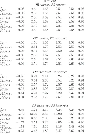
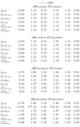
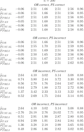
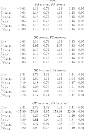
Results for the Kang and Schafer and Tan scenarios are in Tables 1.1, 1.2, 1.3, and 1.4, respectively. When both models are correct, all estimators perform similarly, and all of the doubly robust estimators show negligible Monte Carlo bias when at least one of the models is correctly specified, as expected. Moreover, µbP ROJ and µbenP ROJ for the most part exhibit efficiencies no worse or better than those ofµbORand the other doubly robust estimators on the basis of root mean square error and median absolute error, and in particular dominate the others when the outcome regression model is misspecified but the propensity model is correct, consistent with the basis of their construction. When both models are incorrectly specified,µbU SU ALshows nonnegligible bias, as observed by Kang and Schafer (2007) and Tan (2007); however, use of the “enhanced” propensity model inµben
U SU ALeliminates this behavior. The proposed estimatorsµbP ROJ andµbenP ROJ exhibit the best performance in terms of bias and efficiency when both models are mispecified; in Section 1.7.4, we sketch a heuristic argument suggesting that this behavior is not unexpected. Overall, µben
P ROJ shows the best performance across the range of settings in both scenarios.
Confidence intervals based on sandwich standard errors based on the doubly robust esti-mators for the most part attain nominal coverage except when both models are misspecified in the Kang and Schafer scenario; those forµbP ROJ andµbenP ROJ perform consistently well except in this case. Not unexpectedly, when the outcome regression model is misspecified, confidence intervals based onµbORcan suffer from undercoverage.
1.6 Discussion
draw-backs demonstrated by Kang and Schafer (2007) under model misspecification. We have focused our development on estimation of a single treatment mean in order to demonstrate the approach to developing optimal, doubly robust estimators in Section 1.3 in an accessible context; however, the results are relevant to more complex estimands. In the case where a difference of treatment means is of interest, if one restricts attention to outcome regression models linear in a vector of known functionsg(X)for both treatments, then taking the difference of the optimal, doubly robust estima-tors proposed here will lead to an optimal, doubly robust estimator for the mean difference; see Tan (2006). However, this need not hold in general, e.g., if the posited outcome regression models are nonlinear in their parameters. In this case, it is possible to adapt the approach here to derive directly an optimal, doubly robust estimator for the difference; a sketch of the argument is available Section 1.7.1. The proposed methods may also be adapted to the case of estimation of the parameter in a regression model, where an estimator based on the full data may be derived as the solution to an M-estimating equation; we present such methods in the more general case of monotonely coarsened data in Chapter 2.
Like the stabilized weights discussed by Robins et al. (2000), the enhanced propensity score model proposed in Section 1.4 is an effort to avoid weighting that is too disparate across in-dividuals, leading to instability of the estimator for the mean. In the simple context of estimating a single mean, taking a stabilized weights approach is not possible; accordingly, the proposed en-hanced model provides an effective alternative. Other methods, such as truncating or smoothing estimated propensities, may also yield improved performance. More details regarding this can be found in Section 1.7.2.
It is worth noting that, when the outcome regression model is correct but the propensity model is not, attempting to improve efficiency would be fruitless. Here, the optimal estimator is b
µOR, and the propensity score plays no role; see Tsiatis and Davidian (2007).
It is not necessarily the case that the difference between two optimal estimators for two different treatment means is an optimal estimator for the true difference. Consider the situation where we have observed data (Ri, Yi, Xi), i = 1, . . . , n, where nowRi is a treatment indicator taking values 0 or 1, andYi andXi are response and covariates, respectively. Note that these ob-served data are different from those in this chapter,(RiYi, Yi, Xi). In this setting, we may consider separate estimators for the means for treatments 1 and 0, respectively, as
n−1
n X
i=1 ·
RiYi π(Xi)
− {Ri−π(Xi)}l1(Xi) ¸
, (1.18)
wherel1(X)∈ M1, and
n−1
n X
i=1 ·
(1−Ri)Yi
1−π(Xi) +{Ri−π(Xi)}l0(Xi) ¸
, (1.19)
wherel0(X)∈ M0. Here,M0andM1are spaces of functions depending onX. Alternatively, we may consider an estimator for the difference of means directly, i.e.,
n−1
n X
i=1 ·
RiYi
π(Xi) −
(1−Ri)Yi
1−π(Xi) − {Ri−π(Xi)}l(Xi) ¸
(1.20)
forl(X)∈ M. Consider taking the difference of (1.18) and (1.19) as an estimator of the true mean difference. IfM1 andM0 are linear spaces in known vector-valued functions of X, g1(X)and
Table 1.1: Simulation results based on 1000 Monte Carlo replications for the Kang and Schafer scenario. Sample size is 200. Bias is Monte Carlo bias, RMSE is root mean square error, MAE is median of absolute errors, MCSD is Monte Carlo standard deviation, AveSE is average of sandwich standard errors, Cov is Monte Carlo coverage of 95% Wald confidence intervals, OR is outcome regression, and PS is propensity score. Smallest, median, second largest, and largest standard errors for entries in Table 1.1, 1.2 : BIAS,(0.04, 0.08, 0.39, 5.58); AVESE, (0.0008, 0.004, 0.58, 6.64); COV, (0.006, 0.007, 0.015, 0.015).
Bias RMSE MAE MCSD AveSE Cov
n= 200
OR correct, PS correct
b
µOR −0.06 2.51 1.66 2.51 2.56 0.96
b
µU SU AL −0.06 2.51 1.66 2.51 2.56 0.95
b
µP ROJ −0.07 2.51 1.69 2.51 2.56 0.95
b
µT AN −0.05 2.51 1.68 2.51 2.58 0.95
b
µen
U SU AL −0.06 2.51 1.66 2.51 2.56 0.96
b
µen
P ROJ −0.06 2.51 1.68 2.51 2.58 0.95
OR correct, PS incorrect
b
µOR −0.06 2.51 1.66 2.51 2.56 0.96
b
µU SU AL −0.05 2.53 1.70 2.53 2.57 0.95
b
µP ROJ −0.06 2.50 1.68 2.50 2.56 0.96
b
µT AN −0.05 2.51 1.67 2.51 2.51 0.96
b
µen
U SU AL −0.06 2.51 1.67 2.51 2.62 0.96
b
µen
P ROJ −0.06 2.51 1.70 2.51 2.63 0.96
OR incorrect, PS correct
b
µOR −0.55 3.29 2.14 3.24 3.24 0.93
b
µU SU AL 0.36 3.53 2.33 3.51 3.22 0.94
b
µP ROJ −0.06 2.57 1.72 2.57 2.60 0.95
b
µT AN 0.16 2.88 1.96 2.88 2.81 0.95
b
µen
U SU AL 0.54 3.26 2.27 3.22 3.37 0.94
b
µen
P ROJ −0.04 2.57 1.70 2.57 2.85 0.96
OR incorrect, PS incorrect
b
µOR −0.55 3.29 2.14 3.24 3.24 0.93
b
µU SU AL −5.19 13.26 3.62 12.20 6.54 0.92
b
µP ROJ −0.39 3.58 2.00 3.55 3.28 0.93
b
µT AN −1.77 3.52 2.36 3.05 3.04 0.90
b
µenU SU AL −1.53 3.51 2.29 3.16 5.48 0.91
b
µen
Table 1.2: Simulation results based on 1000 Monte Carlo replications for the Kang and Schafer scenario. Sample size is 1000. Bias is Monte Carlo bias, RMSE is root mean square error, MAE is median of absolute errors, MCSD is Monte Carlo standard deviation, AveSE is average of sandwich standard errors, Cov is Monte Carlo coverage of 95% Wald confidence intervals, OR is outcome regression, and PS is propensity score. Smallest, median, second largest, and largest standard errors for entries in Table 1.1, 1.2 : BIAS, (0.04, 0.08, 0.39, 5.58); AVESE, (0.0008, 0.004, 0.58, 6.64); COV, (0.006, 0.007, 0.015, 0.015).
Bias RMSE MAE MCSD AveSE Cov
n= 1000
OR correct, PS correct
b
µOR −0.03 1.13 0.73 1.13 1.15 0.95
b
µU SU AL −0.03 1.13 0.73 1.13 1.15 0.95
b
µP ROJ −0.03 1.13 0.72 1.13 1.15 0.95
b
µT AN −0.03 1.13 0.73 1.12 1.15 0.95
b
µen
U SU AL −0.03 1.13 0.73 1.13 1.15 0.95
b
µen
P ROJ −0.03 1.13 0.72 1.13 1.15 0.95
OR correct, PS incorrect
b
µOR −0.03 1.13 0.73 1.13 1.15 0.95
b
µU SU AL 0.01 1.72 0.74 1.72 1.28 0.95
b
µP ROJ −0.03 1.13 0.73 1.13 1.15 0.95
b
µT AN −0.03 1.13 0.73 1.13 1.15 0.95
b
µen
U SU AL −0.03 1.13 0.73 1.13 1.15 0.95
b
µen
P ROJ −0.03 1.13 0.73 1.13 1.15 0.95
OR incorrect, PS correct
b
µOR −0.78 1.68 1.18 1.49 1.48 0.91
b
µU SU AL 0.12 1.64 1.09 1.64 1.54 0.93
b
µP ROJ 0.01 1.14 0.73 1.14 1.16 0.95
b
µT AN 0.04 1.27 0.85 1.27 1.26 0.95
b
µen
U SU AL 0.24 1.55 1.02 1.53 1.42 0.92
b
µen
P ROJ 0.02 1.14 0.73 1.14 1.16 0.95
OR incorrect, PS incorrect
b
µOR −0.78 1.68 1.18 1.49 1.48 0.91
b
µU SU AL −18.05 177.45 5.25 176.53 16.60 0.61
b
µP ROJ −1.25 1.78 1.35 1.27 1.24 0.83
b
µT AN −1.69 2.24 1.80 1.47 1.43 0.76
b
µenU SU AL −2.00 2.44 2.08 1.41 1.39 0.69
b
µen
Table 1.3: Simulation results based on 1000 Monte Carlo replications for the Tan scenario. Sample size is 200. Entries are as in Table 1.1. The Tan and Kang and Schafer scenarios are distributionally identical in the “OR correct, PS correct” case. Smallest, median, second largest, and largest standard errors for entries in Table 1.3, 1.4: BIAS, (0.04, 0.08, 0.76, 5.66); AVESE, (0.0008,0.004, 1.59, 9.78); COV, (0.006, 0.007, 0.010, 0.015).
Bias RMSE MAE MCSD AveSE Cov
n= 200
OR correct, PS correct
b
µOR −0.06 2.51 1.66 2.51 2.56 0.96
b
µU SU AL −0.06 2.51 1.66 2.51 2.56 0.95
b
µP ROJ −0.07 2.51 1.69 2.51 2.56 0.95
b
µT AN −0.05 2.51 1.68 2.51 2.58 0.95
b
µenU SU AL −0.06 2.51 1.66 2.51 2.56 0.96
b
µen
P ROJ −0.06 2.51 1.68 2.51 2.58 0.95
OR correct, PS incorrect
b
µOR −0.06 2.51 1.66 2.51 2.56 0.96
b
µU SU AL −0.04 2.55 1.70 2.55 2.59 0.95
b
µP ROJ −0.06 2.51 1.69 2.51 2.56 0.95
b
µT AN −0.05 2.50 1.65 2.50 2.56 0.96
b
µen
U SU AL −0.06 2.51 1.67 2.51 2.57 0.95
b
µen
P ROJ −0.06 2.51 1.68 2.51 2.62 0.95
OR incorrect, PS correct
b
µOR 2.64 4.10 3.02 3.14 3.08 0.88
b
µU SU AL 0.74 3.80 2.44 3.72 3.30 0.93
b
µP ROJ 0.56 2.70 1.76 2.64 2.67 0.95
b
µT AN 0.64 2.79 1.88 2.72 2.72 0.96
b
µen
U SU AL 1.37 3.42 2.33 3.13 3.22 0.91
b
µen
P ROJ 0.52 2.69 1.75 2.64 3.14 0.95
OR incorrect, PS incorrect
b
µOR 2.64 4.10 3.02 3.14 3.08 0.88
b
µU SU AL −2.76 24.18 2.76 24.02 7.71 0.95
b
µP ROJ 0.51 2.91 1.90 2.87 2.80 0.95
b
µT AN 0.94 2.99 1.91 2.84 2.84 0.95
b
µen
U SU AL 1.36 3.28 2.18 2.99 3.65 0.93
b
Table 1.4: Simulation results based on 1000 Monte Carlo replications for the Tan scenario. Sample size is 1000. Entries are as in Table 1.1. The Tan and Kang and Schafer scenarios are distributionally identical in the “OR correct, PS correct” case. Smallest, median, second largest, and largest standard errors for entries in Table 1.3, 1.4: BIAS, (0.04, 0.08, 0.76, 5.66); AVESE, (0.0008,0.004, 1.59, 9.78); COV, (0.006, 0.007, 0.010, 0.015).
Bias RMSE MAE MCSD AveSE Cov
n= 1000
OR correct, PS correct
b
µOR −0.03 1.13 0.73 1.13 1.15 0.95
b
µU SU AL −0.03 1.13 0.73 1.13 1.15 0.95
b
µP ROJ −0.03 1.13 0.72 1.13 1.15 0.95
b
µT AN −0.03 1.12 0.73 1.12 1.15 0.95
b
µenU SU AL −0.03 1.13 0.73 1.13 1.15 0.95
b
µen
P ROJ −0.03 1.13 0.72 1.13 1.15 0.95
OR correct, PS incorrect
b
µOR −0.03 1.13 0.73 1.13 1.15 0.95
b
µU SU AL 0.03 2.07 0.74 2.07 1.32 0.95
b
µP ROJ −0.03 1.13 0.72 1.13 1.15 0.95
b
µT AN −0.03 1.12 0.73 1.12 1.15 0.95
b
µen
U SU AL −0.03 1.13 0.73 1.13 1.15 0.95
b
µen
P ROJ −0.03 1.13 0.73 1.13 1.15 0.95
OR incorrect, PS correct
b
µOR 2.31 2.72 2.32 1.43 1.41 0.63
b
µU SU AL 0.18 1.84 1.14 1.84 1.64 0.93
b
µP ROJ 0.19 1.18 0.76 1.16 1.17 0.95
b
µT AN 0.22 1.23 0.79 1.21 1.21 0.94
b
µen
U SU AL 0.53 1.56 1.03 1.47 1.27 0.89
b
µen
P ROJ 0.18 1.17 0.74 1.16 1.17 0.94
OR incorrect, PS incorrect
b
µOR 2.31 2.72 2.32 1.43 1.41 0.63
b
µU SU AL −17.89 179.88 2.65 178.98 22.60 0.94
b
µP ROJ 0.13 1.25 0.78 1.25 1.20 0.94
b
µT AN 0.89 1.61 1.00 1.35 1.31 0.91
b
µen
U SU AL 0.73 1.47 0.97 1.28 1.27 0.91
b
discussed in Tan (2006). If, however,M1 andM0 are not the same linear space, then this would not necessarily hold, although one could expand these spaces to comprise the space spanned by both
g1(X)andg0(X), as discussed by Tan (2006). Likewise, if any of the spacesM1,M0, orMare nonlinear, that is, e.g., elements ofMare of the arbitrary forml(X, ξ), then again, the difference of optimal (1.18) and (1.19) would not necessarily correspond to the optimal (1.21).
The results in the previous paragraph are relevant whether or not the estimators are doubly robust. We have shown in Section 1.3 that how one estimatesξdetermines double robustness. If we wish to find an optimal, doubly robust estimator for the mean difference, the results in this chapter apply directly if the spaces are linear. Specifically, if one takes M0 and M1 to equal M, then using the strategy in this chapter to estimateξseparately for each mean and taking the difference in resulting estimators would lead to the optimal doubly robust estimator for the difference. However, this does not necessarily hold in the nonlinear case. It is possible to construct an optimal doubly robust estimator for the difference of the form (1.21) by adapting the strategy in this chapter to identify an appropriate estimator forξ. A brief sketch of how one would adpat the strategy for finding the optimal doubly robust estimator for the mean difference of the form (1.21) is given below.
We consider the case where the propensity score is fully specified to demonstrate the idea. Extension to the situation where the a parametric propensity score model is postulated and fitted by binary regression techniques would be handled analogously to the developments in Section 1.3.
As in the standard set-up for the usual causal inference problem in an observational point exposure study, we may conceptualize potential outcomesY0 andY1 corresponding to each treatment, with the observed Y = RY1 + (1−R)Y0. The goal is to estimate the difference ∆ = E(Y1)−E(Y0) based on the observed data under the usual assumption of no unmeasured confounders, namely, that(Y0, Y1)are independent ofRgivenX.
Consider as an estimator for∆
n−1
n X
i=1 ·
RiYi
π(Xi)−
(1−Ri)Yi
1−π(Xi) − {Ri−π(Xi)}l(Xi, b
ξ) ¸
(1.21)
for somel(X, ξ)and estimatorξbforξ. Following the ideas in Section 1.3, we wish to identify a value
ξ∗
opt and an estimatorξbconverging to it such that the asymptotic variance of (1.21) is minimized when the propensity score is correct and such that (1.21) is doubly robust. Using the assumption of no unmeasured confounders, it is straightforward to deduce that the optimal valueξ∗
solution inξto
E
·½
Y1
π0(X) +
Y0
1−π0(X) −l(X, ξ) ¾
π0(X){1−π0(X)}lξ(X, ξ) ¸
= 0,
or equivalently
E
"(
l(1)(X)
π0(X) +
l(0)(X)
1−π0(X) −l(X, ξ) )
π0(X){1−π0(X)}lξ(X, ξ) #
= 0, (1.22)
wherel(k)(X) = E(Y
k | X),k = 0,1, are the true potential outcome means conditional onX. Suppose we posit models lk(X, αk) for E(Yk | X), k = 0,1, where the models lk(X, αk) are possibly nonlinear inαk, and take
l(X, ξ) = l0(X, α0) 1−π(X) +
l1(X, α1)
π(X) , ξ= (α T
0, αT1)T. Suppose we estimateξby solving the estimating equation
n−1
n X
i=1 ·
Ri{1−π(Xi)}
π(Xi) {Yi−l1(X, α1)}+
(1−Ri)π(Xi)
1−π(Xi) {Yi−l0(X, α0)} ¸
lξ(X, ξ) = 0.
(1.23) If the propensity score is correct, π(X) = π0(X), but the models lk(X, αk), k = 0,1, are not, then it is straightforward to show that the left hand side of (1.23) converges to that of (1.22), so that the estimatorξbsolving (1.23) converges in probability toξopt∗ . On the other hand, if the propensity score model is not correct but the modelslk(X, αk)are in the sense that there are valuesα(0)k such thatlk(X, α(0)k ) =l(k)(X),k= 0,1, then the left hand side of (1.23) converges to
E
·
π0(X){1−π(X)}
π(X) {l
(1)(X)−l
1(X, α1)}lξ(X, ξ)
+ {1−π0(X)}π(X) 1−π(X) {l
(0)(X)−l
0(X, α0)}lξ(X, ξ) ¸
,
which equals zero whenξ = ξ0 = (α(0)T0 , α(0)T1 )T, so that ξbconverges in probability toξ0, This shows that the estimator for∆ in (1.21) is doubly robust and achieves the minimum asymptotic variance even if the modelslk(X, αk)forE(Yk|X),k= 0,1, are misspecified.
1.7.2 Enhanced propensity score and stabilized weights
treatment regime in order to avoid weighting that is too disparate across individuals, leading to instability of the mean estimator. In the marginal structural models setting, one takes the estimating equation that one would solve for the associational relationship between regime and mean response and weights it to account for time-dependent confounding. The associational estimating equation is of the form, using Robins’ notation,
n X
i=1
f( ¯Ai){Yi−µ( ¯Ai, ξ)}= 0
for some function f( ¯A). One weights this equation by the product of inverse probabilities that depend on past treatment historyA¯and past covariate historyL¯. Becausef( ¯A) is arbitrary, one can modify its form in the associational estimating equation above to include extra “stabilization” factors, which by definition depend on A¯only. In contrast, in our problem, because we are only estimating a single mean, there is no analogousf( ¯A) and hence no analogous “stabilization fac-tor”. Hence, in our simpler context, we also wish to avoid disparate weights and instability but we cannot use the “stability weights” approach. Accordingly, we chose to adopt the restriction that Pn
i=1Ri/π(Xi,bγ)≈nas an alternative method of achieving less disparate weights; based on our experience, this sum can be very different fromnwhen there are disparate weights. Like the “sta-bilized weights” discussed by Robins et al. (2000), the enhanced propensity score model proposed in Section 1.4 is an effort to avoid weighting that is too disparate across individuals, leading to in-stability of the estimator for the mean. In the simple context of estimating a single mean, taking a “stabilized weights” approach is not possible; accordingly, the proposed enhanced model provides an effective alternative. Other methods, such as truncating or smoothing estimated propensities, may also yield improved performance.
1.7.3 Calculation of asymptotic variances
We provide expressions required to calculate the asymptotic variances of the four esti-mators considered in this chapter: µbOR,µbU SU AL,µbT AN andµbP ROJ. The asymptotic variance of b
µen
U SU AL andµbenP ROJ may be calculated using the same formulæ as forµbU SU AL andµbP ROJ; see below.
regression model by hi = h(Xi, ξ). Let the score corresponding to the propensity score model be Sγi = Sγ(Ri, Xi, γ), and defineSγγi = ∂/∂γTS
γ(Ri, Xi, γ), write hξi = hξ(Xi, ξ), πγi =
πγ(X,, γ),hξξi =∂2/∂ξ∂ξT{h(Xi, ξ)}, andπγγi=∂2/∂γ∂γT{π(Xi, γ)}. Letτ be collection of unknown parameters involved in obtaining the estimators forµ; in particular,τ = (ξT, µ)T forµb
OR,
τ = (γT, ξT, µ)T forbµ
U SU AL,τ = (γT, ξT, cT, µ)T forµbP ROJ, andτ = (γT, ξT, α0, α1, cT, µ)T forµbT AN.
The estimator for τ, bτ, in each case can be obtained by solving a set of M-estimating equations Pni=1ρi(τ) = 0 (Stefanski and Boos, 2002), where the last element of ρi(τ) corre-sponds to the estimating equation forµ. LetAn = n−1
Pn
i=1Ai =n−1 Pn
i=1∂/∂τ{ρi(τ)}, and
Bn = n−1 Pn
i=1ρi(τ)ρTi (τ). Following standard theory, the asymptotic covariance matrix ofbτ can be approximated by the empirical sandwich matrixVn = n−1An−1Bn(A−n1)T. Therefore, the asymptotic variance of the four estimators can be approximated by the last, rightmost diagonal entry of the corresponding matrixVn. We present the form ofρi(τ)andAifor each of the estimators, from which the form ofVnmay be calculated. The desired diagonal entry of Vn may then be obtained numerically, with the required matrix inversion carried out by standard routines.
ForµbOR,ρi(τ)is given by
ρi(τ) =
hξiRi(Yi−hi)
hi−µ
,
andAiis given by
Ai =
D1i 0
hT ξi −1
,
whereD1i =hξξiRi(Yi−hi)−RihξihTξi. ForµbU SU AL,ρi(τ)is given by
ρi(τ) =
Ri−πi
πi(1−πi)πγi
hξiRi(Yi−hi)
Ri
πi(Yi−hi) +hi−µ
,
andAiis given by
Ai =
D1i 0 0
0 D2i 0
whereD1i =
Ri−πi
πi(1−πi)πγγi−
πi(1−πi) + (Ri−πi)(1−2πi) {πi(1−πi)}2
πγiπTγi,D2i=hξξiRi(Yi−hi)−
RihξihTξi,D3i=−Ri
π2 i
(Yi−hi)πTγi, andD4i= µ
1− Ri
πi

hTξi. ForµbT AN,ρi(τ)is given by
ρi(τ) =
Ri−πi
πi(1−πi)πγi
hξiRi(Yi−hi)
Ri(Ri−πi)
π2 i
µ
Yi−α0−α1hi−cT
πγi
1−πi 
Ri(Ri−πi)
π2 i
hi µ
Yi−α0−α1hi−cT1π−γiπ i

Ri(Ri−πi)
π2 i
πγi 1−πi
µ
Yi−α0−α1hi−cT1π−γiπ i

Ri
πiYi−
Ri−πi
πi (α0+α1hi)−c TS
γi−µ
,
and the matrixAiis given by
Ai =
D1i 0 0 0 0 0
0 D2i 0 0 0 0
D3i D4i D5i hiD5i D6i 0
hiD3i 2hiD4i hiD5i h2iD5 hiD6 0
D7i tD4i tiD5 tihiD5 tiD6i 0
D8i D9i D10i hiD10i −Sγi −1 ,
whereD1iandD2iare the same as forµbU SU AL,D3i=D31i−cTD32i,
D31i= −Riπi2−2Ri(1−πi)
π3 i
πTγi
µ
Yi−α0−α1hi−cT πγi
1−πi 
,
D32i= (1−1π i)2
Ri(1−πi)
π2 i
¡
πγγi(1−πi) +πγiπγiT ¢
,
D4i =−α1Ri(1π−2 πi) i
hξi,D5i=−Ri(1π−2 πi) i
,D6i=−Ri(1π−2 πi) i
πγiT
1−πi,
D7i = 1π−γiπ i
D3i+D32i,ti= 1π−γiπ i
,D8i =−Ri
π2 i
πγγi(Yi−α0−α1hi)−cTSγγi,
D9i =−α1Ri−πi πi
hTξi, andD10i=−Ri−πi