The Freight Train Routing Problem

R

ALF

B

ORNDRFER

A

RMIN

F ¨

UGENSCHUH

T

ORSTEN

K

LUG

T

HILO

S

CHANG

T

HOMAS

S

CHLECHTE

H

ANNO

S

CHLLENDORF

The Freight Train Routing Problem

1_{Zuse Institute Berlin (ZIB), Takustr. 7, D-14195 Berlin, Germany{borndoerfer, fuegenschuh, klug, schlechte}@zib.de}

2_{Deutsche Bahn Mobility Logistics AG, Verkehrsnetzentwicklung und Verkehrsmodelle (GSV){thilo.schang, hanno.schuelldorf}@deutschebahn.com}

This work was funded by the German Federal Ministry of Education and Research (BMBF), projectKOSMOS, grant number 03MS640C.

D-14195 Berlin-Dahlem Telefon: 030-84185-0 Telefax: 030-84185-125 e-mail:[email protected] URL:http://www.zib.de

ZIB-Report (Print) ISSN 1438-0064 ZIB-Report (Internet) ISSN 2192-7782

Ralf Borndörfer

_{, Armin Fügenschuh}

_{, Torsten Klug}

_{, Thilo}

Schang

_{, Thomas Schlechte}

_{, and Hanno Schülldorf}

1 Department of Optimization, Zuse Institute Berlin Berlin, Germany

{borndoerfer, fuegenschuh, klug, schlechte}@zib.de 2 Deutsche Bahn Mobility Logistics AG

Verkehrsnetzentwicklung und Verkehrsmodelle (GSV) {thilo.schang, hanno.schuelldorf}@deutschebahn.com

Abstract

We consider the following freight train routing problem (FTRP). Given is a transportation net-work with fixed routes for passenger trains and a set of freight trains (requests), each defined by an origin and destination station pair. The objective is to calculate a feasible route for each freight train such that a sum of all expected delays and all running times is minimal. Previous research concentrated on microscopic train routings for junctions or inside major stations. Only recently approaches were developed to tackle larger corridors or even networks. We investigate the routing problem from a strategic perspective, calculating the routes in a macroscopic trans-portation network of Deutsche Bahn AG. Here macroscopic refers to an aggregation of complex real-world structures are into fewer network elements. Moreover, the departure and arrival times of freight trains are approximated. The problem has a strategic character since it asks only for a coarse routing through the network without the precise timings. We give a mixed-integer non-linear programming (MINLP) formulation for FTRP, which is a multi-commodity flow model on a time-expanded graph with additional routing constraints. The model’s nonlinearities are due to an algebraic approximation of the delays of the trains on the arcs of the network by capacity restraint functions. The MINLP is reduced to a mixed-integer linear model (MILP) by piecewise linear approximation. The latter is solved by a state of the art MILP solver for various real-world test instances.

1998 ACM Subject Classification F.2.2 G.1.6 G.2.2 G.2.3 J.7 K.6.1

Keywords and phrases freight train routing, capacity restraint functions, multi-commodity flows, mixed-integer linear and nonlinear programming

1

Introduction

The rail transport volume in Germany increases for years, while corresponding expansion of the infrastructure is rather small, since the changes of the infrastructure are always capital-intensive and long term projects. Germany as a transit country in central Europa faces a great challenge in the next years. In particular, this applies for the rail freight traffic. Recent estimates assume an increase up to 80 percent by 2025 [IFMO-Studie, 2005]. To make best use of the infrastructure, Deutsche Bahn has to identify the bottlenecks of the network. One important part is to find routes that avoid the occurrence of bottlenecks. Therefore, it is necessary to analyze the existing network to estimate and make best use of the available capacity. In this context the Deutsche Bahn AG focuses on the railfreight train routing on a strategic planning level in a simplified (macroscopic) transport network. The major aim is to determine routes for freight trains by taking into account the available railway infrastructure and the already planned and invariant passenger traffic.

The routing of freight trains is quite different from passenger trains since departure and arrival time windows are less strict and routes are not limited by several intended intermediate stops. Nevertheless, passenger and freight trains in Germany share the same infrastructure, and therefore we have to consider the railway system as a whole including railway passenger transport and infrastructure to provide reasonable strategic prospectus.

Almost all national railway systems in Europe consist of three business divisions shown as columns in Figure 1, i.e., passenger traffic, freight transportation, and infrastructure department (including service). In the middle the (tool) chain for planning freight trains is idealized. Railway infrastructure (from network design), predefined passenger transportation (from line planning or even timetabling) is given as input as well as forecasting results for future freight traffic demand. Based on that data a reasonable traffic flow for the freight trains covering the forecasted demand is determined, which is the topic of this paper.

passenger infrastructure freight

forecasting single car routing network design freight train routing track allocation line planning timetabling level strategic tactical

Figure 1Idealize planning process of the concern model with focus on the freight train routing problem in a segregated railway system, see e.g., [Schülldorf, 2008].

As a result the necessary train paths for the freight trains have to be scheduled in time through the railway network and integrated into the annual railway timetable. Many recent contributions from research concentrate on the subsequent step, the timetabling or track allocation which assumes inter alia freight train routes as an input. Caimi [Caimi, 2009] presents a top-down approach and uses it to handle the complete Swiss network by a priori decomposition of the network into different zones. In contrast to that, Borndörfer et al. [Schlechte et al., 2011] present a bottom-up approach to define a macroscopic railway model based on microscopic simulations. A similar approach can be found in Kettner, Sewcyk, and Eickmann [Kettner et al., 2003]. There an automated generation of macroscopic data from a microscopic basis is described for the Austrian Federal Railways (ÖBB).

Besides the special application context, our problem has similarities to the broader class ofnetwork designproblems, see Balakrishnan et al. [Balakrishnan et al., 1997] for a general survey. A framework for a general class of network design problems is presented in Kim and

u x y v u x y v u x y v

Figure 2Balanced and unbalanced flows.

Barnhart [Kim and Barnhart, 1997] and applied to the blocking problem in railroad traffic in the US, see Barnhart, Jin, and Vance [Barnhart et al., 2000]. Integrated service network design for rail freight transportation in the US is considered in Zhu, Crainic, and Gendreau [Zhu et al., 2009], and Ahuja et al. [Ahuja et al., 2007, Jha et al., 2008].

Deutsche Bahn, the largest German railway company, primarily offers two products to industrial customers that want to transport freight via rail. Typically large customers order block-trains of about 20 to 40 cars. In this case, Deutsche Bahn, i.e., DB Schenker, as the operator can pull such a complete train by a locomotive from origin to destination. That is a direct freight transportation offer with a fixed train composition. Small customers on the other hand order only 1 to 5 cars. In such cases it is too expensive to pull these groups of cars each by a single locomotive through the network. Instead the cars are only pulled to the next classification yard. There they are grouped with the cars from other customers, and then as new trains pulled to the next classification yard. There the trains are disassembled, and the cars are again re-grouped with others until each car has reached its final destination. This second freight transportation product of DB gives rise to a natural network design question, i.e., where are the classification yards located and how to route between them. Fügenschuh et al. [Fügenschuh et al., 2008, Fügenschuh et al., 2009] discuss the whole system ofsingle wagon freight transportation, show the positive effect of bundling cars, and compare the problem to other freight transportation concepts mentioned in the literature, e.g., therailroad blocking problem in the US or Canada.

The railroad blocking problem can be formulated as a very large-scale, multi-commodity, flow-network-design and routing problem with billions of decision variables, see [Jha et al., 2008] and [Barnhart et al., 2000]. [Ahuja et al., 2007] presented an algorithm using an emerging technique known as very large-scale neighborhood search to support major US railway companies that transfers millions of cars over its network annually. The authors report that their heuristic approach is able to solve the problem to near optimality using one to two hours of computer time on a standard workstation computer.

In the case of road traffic [Köhler et al., 2009] present mathematical theory on flow depended cost functions. A major difference is that in road traffic the routing is decentralized, arbitrarily partitionable, and assumed to be selfish. In contrast to that railway systems are centralized and we are aiming for a system optimum. In addition the train flow can not be partitioned arbitrarily and thus the routing and timetable is a more rigid system in comparison to the flow of cars.

We investigate the routing problem from a strategic perspective, calculating the routes in a macroscopic transportation network. In this terms macroscopic means complex structures are aggregated into fewer elements and the departure and arrival times of freight trains are approximated. The problem has a strategic character since it asks only for a rough routing through the network without the precise timings, i.e., in particular most of the input data consists only of coarse estimates. In order to achieve a balanced network utilization we propose a nonlinear optimization approach. Consider the simple situation shown in Figure 2

with two possible choices to route trains from nodeutov. Let us assume that the path via xis much shorter than the detour viay. In such a case linear models will tend to route all

trains fromutov on the shortest path as long as the capacity is not violated - idealized

illustrated as thick blue flow in the middle. An optimization model utilizing a nonlinear objective function results in an adequate balanced solution as shown on the right hand of Figure 2. The main benefit is to identify automatically bottlenecks of the railway network and support the network design task in a quantified way. The details of this nonlinear delay function are presented in the following.

The paper is organized as follows: Section 4 will describe an mixed-integer nonlinear model based on capacity restraint functions for the freight train routing problem (FTRP). We utilize linearization techniques to solve the mixed-integer nonlinear model by using a standard MIP solver. Finally, we will present computational results for data from our project partner Deutsche Bahn AG in Section 6.

2

Capacity Restraint Functions

Modeling railway capacity is technically very complex and hence the prediction of congestion and waiting times is a major challenge. Nevertheless, the crucial relation is that there is almost no waiting time as long the mixture of allocated trains can be handled by the infrastructure capacity. Once the capacity limit is reached congestion starts and smooth operation is not possible anymore. The closer it gets to the capacity limit, the more delay occurs for each train. As soon as the number of trains goes further beyond the capacity limit, the average delay for each train grows even faster. A way to model the functional relationship between the number of trains passing a certain infrastructure (an arc in the network model) is to introduce a capacity restraint (CR) function. These functions are designed to give a reasonable measure of the expected average delay. One of the earliest appearence of CR-function in the literature is due to Irwin et al. [Irwin and Cube, 1962]. Wohl [Wohl, 1968] uses CR-functions to describe the travel performance or travel time and delay as a function of the flow using properties of the infrastructure and its capacity during the tri distribution and assignment phases of a travel forecasting process. Most applications of CR-functions are tailored to road traffic. Only recently, Lieberherr and Pritscher [Lieberherr and Pritscher, 2012] use CR-functions in railway passenger transport. To the best of our knowledge, our work is the first application of CR-functions to railway freight transport.

Letnbe the number of trains on a track, then the congestion or delay is defined as:

τ 1 +α

_n

κγ

β!

, α, β_∈[0,_∞[, γ_∈]0,_∞[, (1)

where the running time τ and the capacity κ depends on the track. This function is an

undamped variant of the CR-function presented in [Lieberherr and Pritscher, 2012]. In this work a justification for the exponential growth of the CR-function is also given. α, β, γ are

parameters to control the shape of the CR-function. αcould be interpreted as the multiple

of the running time that a train gets if the capacity limit is reached. We chooseα= 1, which

means we must pay the running time of a train if we reach the capacity. γcould be used to

scale the capacity, i.e., to keep an amount of reserve capacity. Since we do not want to keep any capacity we chooseγ= 1. This simplifies the CR-function to

τ1 +n κ

β

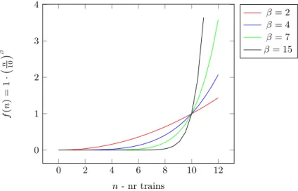
0 2 4 6 8 10 12 0 1 2 3 4 n- nr trains f ( n ) = 1 · n 10 β β= 2 β= 4 β= 7 β= 15

Figure 3CR-Functions withka= 10, τa= 1 andβ∈ {2,4,7,15}

β controls the rapidness of the penalization. A large value for β means a big slope near

the capacity. A small leads to a moderate slope. Since the running time is already in the objective function we take only the surplus as waiting time cost

f(n) =τn κ

β

. (3)

We use function (3) to estimate the congestion on each track.

3

Input Data and Problem Description

The transportation network is given as a directed graphGI = (_VI_,AI). Anode _{v ∈ V}I represents a station, a junction or some other infrastructure element where train routes can start, branch or end. There is a directed arc between two nodes if the corresponding infrastructure elements are connected by a track.

We consider a standard day with the assumption that the demand of the previous and the next days are equal. The day is partitioned into a small number of time slices, four in our study. They are arranged in a cyclic order such that a train at the end of the day (last time slice) can go on at the begin of the day (first time slice). The set of time slices is denoted by

S. Letlsbe the time span of time slice s. For each track a capability value κa, a∈ AI is given that describes the approximated number of trains that could use the track over the whole day. The trains are classified into a set of standardtrain types T with specific track

dependent characteristics and running dynamics. For each arca_{∈ A}I_,l

a denotes the length of the arc andτt,a defines the running time of train typet∈ T.

The freight train demand is given by a set of trains R. Atrain r_{∈ R}is associated with

an origin station, an destination station, a starting time slice, and a train typetr. The arrival time slice is not restricted. It is required that the paths are not far apart form the shortest and fastest paths. Therefore, the running time and length of a possible routing is restricted to a multiple of the fastest or shortest path, denoted as ∆r

time and ∆rdist, respectively. In our

study we use 150 percent. The resource consumption of the passenger traffic is given as the number of trains per time slice.

A request or train will travers the infrastructure graph and at each node can decide to which node to drive next. In reality, however, there are further turning restrictions imposed

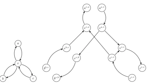
v a b c va,v vv,a vb,v vv,b vv,c vc,v av,a _aa,v bb,v bv,b cv,c cc,v

Figure 4Construction of the expanded graph to handle turning restrictions. In this example, turning frombvia v toc(and vice versa) is forbidden. Also a u-turn froma and frombis not allowed. HenceTF :={(b, v, c),(c, v, b),(a, v, a),(b, v, b)}.

at the nodes of the network. Simply speaking, sharp turning angles are either forbidden or come with extra cost. Anez et al. [Anez et al., 1996] already discusses this problem for street networks with turning restrictions and models it via a dual graph representation to save some arcs and nodes. Since we have further constraints on the flow that would be complicated to formulate on the dual graph we will stick to the original infrastructure graph and expand it.

We assume that two disjoint sets are given. The first setTF consists of all node triples (u, v, w) with (u, v),(v, w)∈ AI such that the node sequence_{u, v, w}is forbidden for all trains.

In general the triple (u, v, u) for (u, v)_{∈ A}I _{belongs to this set, since it is not allowed to} leave a station in the direction from which it was entered. The second setTRconsists of all node triples (u, v, w) with (u, v),(v, w)_{∈ A}I _{such that a turning from (u, v) to (v, w) inv} comes with extra costcu,v,w in the objective function. In some cases the triple (u, v, u) for (u, v)∈ AI belongs to this set, if it is possible to shunt the locomotive from one end of the train to the other. In this case the train can revert its direction and leave the stationv in

the same direction where it came from.

Denote by deg(v) the degree of nodev, i.e., the sum of all arcs entering or leaving node v. We construct an expansion of graphGI _{= (}

VI_,

AI_{) that is capable of handling turning} restrictions. For each nodev∈GIwe introduce 2 deg(_v) many copies. We denote these copies byvv,w_andvw,v_{, for each (v, w),(w, v)}

∈ AI_{. We introduce an arc (v}u,v_{, v}v,w_{) between two} new nodes if and only if (u, v, w)6∈ TF. This are additional arcs with length zero and running timecu,v,w if and only ifTR contains (u, v, w). Each arca= (u, v)∈ AI becomes (uu,v, vu,v) in the expanded graph and has the same properties as the corresponding arc inGI_{. An} example is shown in Figure 4. The so-constructed graph is denoted byGx= (_Vx_,Ax).

For the strategic planning we have no information about the actual schedule of trains using a common network element and running in the same time slice. Therefore, we define for each track the congestion cost functionfa : 2R→R+that depends on the train set using the corresponding track. This measures the expected delay. The main part of this function is the in the last section described CR-function. The other parts are the running time and the lengths.

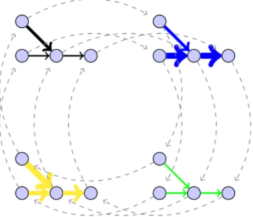
The task is to find a route for each train inGx_{. The determined routes should minimize the} sum of all expected delays and the subordinate criteria running time and length. Capacity

Figure 5Example of a time extended graph created out of a infrastructure graph of four nodes with four time slices. The color depict the different time slices and the thickness of the arcs illustrate the predefined load of passenger traffic.

limitations of the arcs are implicitly handled by the congestion function, i.e., potential conflicts of trains using the same infrastructure element result larger congestion values. By minimizing the sum of delays we increase the chance that timetables with small delays can be produced.

4

A Mixed-Integer Nonlinear Model for the FTRP

To model the problem we construct a time slice expanded graph G. To the best of our

knowledge the time-expansion of a graph was first introduced by Ford and Fulkerson [Ford and Fulkerson, 1958] in their analysis of maximal dynamic flows. Since then, many real-world problems have been formulated as time-space network models, see Kennington and Nicholson [Kennington and Nicholson, 2010] for a survey.

For each node v∈ Vx _{and for each arca}

∈ Ax_{we have a copy for each time slices} ∈ S

inG. Thus, the time expanded graphGcontains_|S|copies of the original graphGx _and additional transition arcs, defined as follows: Letvs1, vs2, . . . vsk be the copies of nodev in

the time expanded graph andk=|S|, then arcs (vsi, vsi+1) fori= 1, . . . , k−1 and (vsk, vs1)

represent the transition from one time slice to another in v. We denote the nodes and arcs

of the time slice expanded graph G by V and A. The length and running times of the

non-transition arcs are taken fromGx_{. Transition arcs have length zero and the running time} is defined by the time span of the time slice the arc start from. We denote the given number of passenger trains traversing arc awith ρa. The capabilitiesκa, a∈ Ax are distributed over the time slices in dependence of the time slice lengths.

For each request the o(r)∈ V is the origin node in the time expanded graph. Since the

arrival time slice of a request is not restricted we have a destination node for each time slice. The set of destination nodes of requestris denoted byDr.

Based on the time expanded graph we model the FTRP as a multi-commodity arc flow problem. Therefor, we introduce a binary decision variablexr

a for each arca∈ Aand each

r∈ R. The variable is one if and only if trainruses arca, otherwise the variable is zero.

Letx_{∈ {}0,1_}A×R be the vector of these variables.

The objective function contains the total nonlinear congestion cost for each track and the sum of all running times and lengths. λtime, λrunning, λlengthare the cost values for each part.

τa is the average running time of this arc over all train types. min λwait X ∀a∈A τa P r∈Rxra+ρa κa β | {z } congestion cost +λtimeX r∈R X a∈A xraτt,a | {z } running time +λlengthX r∈R X a∈A xrala | {z } length

The constraints are

X a∈δ+(v) xra− X a∈δ−₍v) xra= 0 ∀r∈ R ∀v∈ V \(o(r)∪D(r)) (4) X a∈δ+(o(r)) xr a= 1 ∀r∈ R (5) X v∈Dr X a∈δ−₍v) xra= 1 ∀r∈ R (6) X a∈A(s) τt,axra≤τslen ∀s∈ S ∀r∈ R (7) X a∈A laxra≤∆rdist ∀r∈ R (8) X a∈A τt,axra≤∆rtime ∀r∈ R (9) xra∈ {0,1} ∀a∈ A ∀r∈ R (10)

We have the common flow constrains for each train: the outflow must be one at the origin (5); the inflow must be one at exactly one of the destination node copies in the time expanded graph (6); and at the remaining nodes flow conservation (4) is required. We have constraints for the length and running time restrictions (8) (9). A train must change to the succeeding time slice at least if the running time is larger than the time span of the time slice (7).

5

Solution Approach

The MIP model contains a binary variable for each arc and train. In terms of the considered instances of Deutsche Bahn AG this are up to 25 Million binary variables. Setting up such a model consumes an enormous amount of computer memory, and solving such model takes a daunting amount of time. In the following we describe our efforts to reduce the resource demand. We focus on presolving, that is, we only generate those parts of the model that are really necessary because they contain an optimal solution, and remove all the others. Furthermore we describe the linearisation of the nonlinear objective function that transforms the MINLP to a MIP.

5.1 Presolving

For the preprocessing we analyse for each train the network and try to find arcs and nodes that are not a part of a feasible solution.

Obviously, all ingoing arcs of the origin node and all outgoing arcs of destination nodes can be ignored. The running time restriction is much less than 24 hours for all trains. Therefore we assume that a train cannot enter its starting time slice again by running over all four time slices. This means all trainsition arcs into the starting time slice of a train could be ignored.

The major part of the preprocessing is to reduce the network for a train to the subset of arcs and nodes that are element of a path from the origin to one of the destinations and observe the length and running time restriction. To find the relevant arc and node subsets we construct a shortest path tree from the origin and one tree from the destination node. We could stop in the leafs of the tree if the distant from the root to the leaf is bigger than the length restriction. Then for each node we check if the distant to the origin node plus the distant to the destination node is less that the length restriction. If the sum is less than the length restriction the node could be in a feasible solution. Otherwise the node cannot be an element of an feasible path without violating the length restriction. We do the same for the running time restriction. Determine for each train its relevant subset of arcs we get a significant reduction of flow variables.

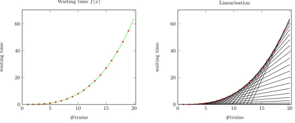
5.2 Linearization of the Objective Function

In order to solve theFTRPwith standard MIP solvers we linearize the nonlinear terms of the objective function. We apply the linearization technique used in [Fügenschuh et al., 2010]. Since it is not allowed to split trains, the total number of trains traversing an arc a is

always integer. Hence, we need only the function values for feasible integer input values. We introduce for each arcaan artificial continuous variableya. Without loss of generality we assume the total number of trains per arc is bounded by some valueN, then the constraints:

Γ1(m) X r∈R xr a+ρa ! + Γ2(m) ≤ya ∀a∈ A ∀m∈ {0,1, . . . , N}

describe the convex hull of all feasible integer points. Γ1(m) is the slope and Γ2(m) the

y-inersection of the linear function throw the points (m, f(m)) and (m₋1, f(m₋1)). The

slope is defined by Γ1(m) =fa(m)−fa(m−1) = ατ κβ (m+ρa) β −(m₋1 +ρa)β (11)

and the y-intersection by

Γ2(m) =fa(m)−Γ1(m)m (12) An example how this linearisation looks like depicts figure 6. The transformed cost function is: min λwait X ∀a∈A yala | {z } congestion cost +λtimeX r∈R X a∈A xraτt,a | {z } running time +λlengthX r∈R X a∈A xrala | {z } length (13)

6

Computational Results

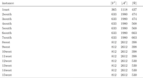
We used IBM Cplex 12.4 to evaluate our solution approach. The software was running on a Linux system with 48 GB main memory and an Intel Xeon CPU with four cores running at 3.2GHz each. Our industrial partner provides us data with the macroscopic railway network of whole Germany and a corresponding demand forecast. Based on this we consider 15 instances from networks of three geographical areas(figure 7). Table 1 gives the sizes in terms

0 5 10 15 20 0 20 40 60 #trains w aiting time Waiting timef(x) 0 5 10 15 20 0 20 40 60 #trains w aiting time Linearisation

Figure 6Linearisation of a CR-Function where only integer points are interesting.

(a)south (b)east (c)west

Figure 7Macroscopic infrastructure graphs for three geographical areas.

of number of nodes (VI), of arcs (_AI), and of trains (_R) for all instances. From a pool of possible requests we choose different subsets of request for he specific area.

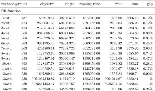
In order to get the instance manageable for the MIP solver the preprocessing reduce the problem size to 5% of the original problem. Table 2 contains the results of the preprocessing.

The computational results are shown in table 2. For this model the mip solver could find a solution with a gap less than one percent in less than an our. Only for some of the west instances the solving of root lp takes over an hour.

instance |VI | |AI | |R| 1east 365 1118 437 2south 633 1980 474 3south 633 1980 474 4south 633 1980 568 5south 633 1980 568 6south 633 1980 663 7south 633 1980 663 8west 812 2612 398 9west 812 2612 398 10west 812 2612 398 11west 812 2612 398 12west 812 2612 530 13west 812 2612 530 14west 812 2612 530 15west 812 2612 530

Table 1Magnitude of the considered macroscopic railway networks.

before preprocessing after preprocessing

instance |V| |A| |V| |A|

1east 3908528 9019680 341652(9%) 666570(7%) 2south 7508160 18023376 451480(6%) 938163(5%) 3south 7508160 18023376 442732(6%) 920964(5%) 4south 8997120 21597632 524980(6%) 1088856(5%) 5south 8997120 21597632 503344(6%) 1042745(5%) 6south 10501920 25209912 600484(6%) 1245681(5%) 7south 10501920 25209912 574064(5%) 1188863(5%) 8west 8316608 20049648 449212(5%) 952603(5%) 9west 8316608 20049648 514156(6%) 1091849(5%) 10west 8316608 20049648 484528(6%) 1024462(5%) 11west 8316608 20049648 451944(5%) 957397(5%) 12west 11074880 26699280 519820(5%) 1095987(4%) 13west 11074880 26699280 617744(6%) 1310090(5%) 14west 11074880 26699280 689764(6%) 1463058(5%) 15west 11074880 26699280 613648(6%) 1298374(5%)

Table 2Compare the dimension of the graph before and after preprocessing. The first and second column is the theoretical number of nodes and arcs without preprocessing. In the third and fourth column are the number of nodes and arcs after preprocessing. The percentage within the brackets are the relative size to the theoretical dimension.

instance #trains objective length running time wait time gap CR-function 1east 437 1666019.44 49206.579 1874912.00 1603.68 3606.43 0.12% 2south 474 2508037.38 59190.876 2291466.00 2432.04 3586.23 0.12% 3south 474 2170813.74 56143.089 2163687.00 2099.00 3593.85 0.12% 4south 568 3345086.86 69041.669 2676385.00 3256.34 3564.35 0.39% 5south 568 2496226.82 66976.321 2602786.00 2409.95 3573.69 0.34% 6south 663 3841995.48 78984.324 3063357.00 3740.42 3571.34 0.45% 7south 663 4204800.11 77808.725 3012223.00 4104.90 3575.86 2.60% 8west 398 1128753.73 30041.969 1155864.00 1090.38 3585.65 0.74% 9west 398 1249467.07 35040.147 1350219.00 1204.65 3584.23 0.47% 10west 398 1128187.78 33933.649 1306450.00 1084.82 3583.27 0.28% 11west 398 1140789.54 32096.015 1228716.00 1099.97 3580.18 0.17% 12west 530 1607809.14 39143.028 1505059.00 1557.84 3169.74 0.00% 13west 530 5061067340.87 41671.719 1583327.00 5061014.67 3582.41 -% 14west 530 6925661452.47 44908.767 1724531.00 6925604.18 3580.66 -% 15west 530 1595650.32 43869.209 1686440.00 1539.66 3582.62 0.26%

Table 3Computations with one hour time limit using the CR-function withβ= 3 as congest cost. The table contains the number of train in the second column. Column 3 to 6 containing the objective function value and the total length, the total running time and the total waiting time. The second last column contains the running time of CPLEXand the last the gap after 1 hour.

Acknowledgement

This work was funded by the German Federal Ministry of Education and Research (BMBF), projectKOSMOS, grant number 03MS640C.

References

Ahuja et al., 2007 Ahuja, R. K., Jha, K. C., and Liu, J. (2007). Solving real-life railroad blocking problems. Interfaces, 37(5):404–419.

Anez et al., 1996 Anez, J., Barra, T., and Perez, B. (1996). Dual graph representations of transport networks. Transportation Research, 30(3):209–216.

Balakrishnan et al., 1997 Balakrishnan, A., Magnanti, T. L., and Mirchandani, P. (1997). Network design. In Dell’Amico, M., Maffioli, F., and Martello, S., editors, Annotated bibliographies in combinatorial optimization, pages 311–334. John Wiley & Sons Inc.

Barnhart et al., 2000 Barnhart, C., Jin, H., and Vance, P. H. (2000). Railroad blocking: A network design application. Oper. Res., 48(4):603–614.

Caimi, 2009 Caimi, G. (2009). Algorithmic decision support for train scheduling in a large and highly utilised railway network. PhD thesis, ETH Zurich.

Ford and Fulkerson, 1958 Ford, L. and Fulkerson, D. (1958). Constructing Maximal Dy-namic Flows from Static Flows. Operations Research, 6:419 – 433.

Fügenschuh et al., 2008 Fügenschuh, A., Homfeld, H., Huck, A., Martin, A., and Yuan, Z. (2008). Scheduling Locomotives and Car Transfers in Freight Transport. Transportation Science, 42(4):1 – 14.

Fügenschuh et al., 2009 Fügenschuh, A., Homfeld, H., and Schülldorf, H. (2009). Single car routing in rail freight transport. In Barnhart, C., Clausen, U., Lauther, U., and Möhring, R., editors,Dagstuhl Seminar Proceedings 09261, Schloss Dagstuhl – Leibniz-Zentrum für Informatik, Deutschland.

Fügenschuh et al., 2010 Fügenschuh, A., Homfeld, H., Schülldorf, H., and Vigerske, S. (2010). Mixinteger nonlinear problems in transportation applications. In et al., H. R., ed-itor,Proceedings of the 2nd International Conference on Engineering Optimization (+CD-rom).

IFMO-Studie, 2005 IFMO-Studie (2005). Zukunft der Mobilität – Szenarien für das Jahr 2025. Technical report, Institut für Mobilitätsforschung.

Irwin and Cube, 1962 Irwin, N. and Cube, H. V. (1962). Capacity restraint in multi-travel mode assignment programs. Highway Research Board Bulletin, 347:258 – 287.

Jha et al., 2008 Jha, K. C., Ahuja, R. K., and Şahin, G. (2008). New approaches for solving the block-to-train assignment problem. Networks, 51(1):48–62.

Kennington and Nicholson, 2010 Kennington, J. and Nicholson, C. (2010). The Uncapac-itated Time-Space Fixed-Charge Network Flow Problem: An Empirical Investigation of Procedures for Arc Capacity Assignment. INFORMS Journal on Computing, 22(2):326 – 337.

Kettner et al., 2003 Kettner, M., Sewcyk, B., and Eickmann, C. (2003). Integrating mi-croscopic and mami-croscopic models for railway network evaluation. InIn Proceedings to the European Transport Conference.

Kim and Barnhart, 1997 Kim, D. and Barnhart, C. (1997). Transportation service network design: Models and algorithms. In Wilson, N. H. M., editor,Proc. of the Seventh Inter-national Workshop on Computer-Aided Scheduling of Public Transport (CASPT), Boston, USA, 1997, volume 471 ofLecture Notes in Economics and Mathematical Systems, pages 259–283. Springer-Verlag, Berlin, Heidelberg.

Köhler et al., 2009 Köhler, E., Möhring, R. H., and Skutella, M. (2009). Traffic networks and flows over time. In Lerner, J., Wagner, D., and Zweig, K. A., editors,Algorithmics of Large and Complex Networks: Design, Analysis, and Simulation, volume 5515 ofLecture Notes in Computer Science, pages 166–196. Springer.

Lieberherr and Pritscher, 2012 Lieberherr, J. and Pritscher, E. (2012). Capacity-restraint railway transport assignment at SBB-Passenger. InProceedings of the 12th Swiss Transport Research Conference.

Schlechte et al., 2011 Schlechte, T., Borndörfer, R., Erol, B., Graffagnino, T., and Swarat, E. (2011). Micro-macro transformation of railway networks. Journal of Rail Transport Planning & Management.

Schülldorf, 2008 Schülldorf, H. (2008). Optimierung der Leitwegeplanung im Schienen-verkehr. Diploma thesis, Technische Universität Darmstadt.

Wohl, 1968 Wohl, M. (1968). Notes on transient queuing behavior, capacity restraint func-tions, and their relationship to travel forecasting. Papers in Regional Science, 21(1):191 – 202.

Zhu et al., 2009 Zhu, E., Crainic, T. G., and Gendreau, M. (2009). Integrated service net-work design in rail freight transportation. Research Report CIRRELT-2009-45, CIRRELT, Montréal, Canada.