On Energy-Efficient Trap Coverage in Wireless Sensor Networks
Junkun Li† Jiming Chen† Shibo He† Tian He‡ Yu Gu§ Youxian Sun† †State Key Lab. of Industrial Control Technology, Zhejiang University, China
‡Computer Science and Engineering, University of Minnesota, USA
§Pillar of Information System Technology and Design, Singapore University of Technology and Design, Singapore.
{lijunkun, ferrer}@zju.edu.cn,{jmchen, yxsun}@iipc.zju.edu.cn, [email protected], [email protected] Abstract—In wireless sensor networks (WSNs), trap coverage
has recently been proposed to tradeoff between the availability of sensor nodes and sensing performance. It offers an efficient framework to tackle the challenge of limited resources in large scale sensor networks. Currently, existing works only studied the theoretical foundation of how to decide the de-ployment density of sensors to ensure the desired degree of trap coverage. However, the practical issues such as how to efficiently schedule sensor node to guarantee trap coverage under an arbitrary deployment is still left untouched. In this paper, we formally formulate theMinimum Weight Trap Cover Problem and prove it is an NP-hard problem. To solve the problem, we introduce a bounded approximation algorithm, calledTrap Cover Optimization(TCO) to schedule the activation of sensors while satisfying specified trap coverage requirement. The performance of Minimum Weight Trap Coverage we find is proved to be at mostO(ρ)times of the optimal solution, where
ρ is the density of sensor nodes in the region. To evaluate our design, we perform extensive simulations to demonstrate the effectiveness of our proposed algorithm and show that our algorithm achieves at least 14% better energy efficiency than the state-of-the-art solution.
Keywords-trap coverage; energy-efficient; scheduling; wire-less sensor networks
I. INTRODUCTION
While recent advances in wireless communication and hardware device have posed a bright blueprint for Wireless Sensor Network (WSN) applications in a large range of fields including military affairs, health care and environment surveillance [1], [2], most practical implementations are restricted to small-scale experiments or applications with dozens or hundreds of sensors. One of the major reason for such relatively small scale deployment is the prohibitively high cost of deploying thousands/millions of sensor nodes for large scale applications. Consequently, designing a sen-sor network where the number of sensen-sor nodes does not increase quickly (e.g., exponentially) with the deployment size while maintaining desired system performance is a fundamental challenge.
Partial coverageis introduced in [3] to address the limited quantity of sensor nodes in large-scale applications, as it is prohibitively expensive to guarantee the full coverage of the Region of Interest (RoI) [4]–[6]. Partial coverage
allows coverage holes [7] and its quality of coverage is mainly indicated by the ratio of uncovered area to the whole
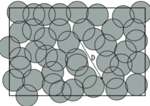
Figure 1. An example of trap coverage,Dis the largest diameter among all coverage holes.
region [3], [8], [9]. By adopting partial coverage scheme, a significant number of sensor nodes could be saved and thus scale well with the network size. However, for the partial coverage, it is difficult to evaluate the actual network performance by the ratio of uncovered area as the size of coverage holes could be extremely large or even unbounded. For applications such as intrusion detection, this implies that the moving target could travel an arbitrarily long distance and time in certain area of the RoI without being detected. Therefore, the simple partial coverage has a very narrow spectrum of practical applications that has well recognized by many researchers.
To tradeoff the scalability and network performance, P. Balister et al. recently propose a new kind of coverage, calledtrap coverage [10], based on the concept ofpartial coverage. Intrap coverage, the size of each coverage hole is incorporated as the indicator of quality of sensing. For the coverage hole, its size is indicated by its diameter D, which is defined as the largest Euclidean distance between any two points in the coverage hole. A set of sensor nodes is said to provide D-Trap Coverage to the RoI A, if the diameter of every coverage hole in A is smaller or equal to D. Although there may exist lots of coverage holes in the network according to this definition, the largest area of coverage holes is no more than πD2. An example of
trap coverage is illustrated in Fig. 1. A target is trapped in a coverage hole as it will be detected within a maximal moving distance ofD. Compared with the partial coverage which takes coverage ratio as an indicator, trap coverage
guarantees the quality of coverage in the worst case. By
2011 32nd IEEE Real-Time Systems Symposium
carefully controlling the parameterD, network performance such as connectivity or delay of detecting intrusions can be ensured intrap coverage.
P. Balisteret al.for the first time study the trap coverage of randomly deployed sensor networks. They consider the fundamental problem of how to design reliable and explicit deployment density required to achieve D-trap coverage. Their work is concerned with conceptual network design, however, practical implementation scheme such as how to si-multaneously guarantee trap coverage and energy efficiency is left uninvestigated. As sensor nodes could be deployed in an arbitrary manner, the required number of sensor nodes to ensureD-trap coverageis usually more than the optimal value.
In this paper, we fill in this gap by considering the energy-efficient scheduling of sensor nodes in the randomly deployed sensor networks to achieve D-trap coverage for the first time. In fact, this problem is extremely difficult and we have proved that it is an NP-hard problem. To effectively solve this problem, we design an approximation algorithm calledTrap Cover Optimization. Specifically, the main intellectual contributions of this work are as follows:
1) To the best of our knowledge, we are the first to study how to schedule the activation of sensors to maximize network lifetime while D-trap coverageis ensured in the randomly deployed sensor networks. The problem of scheduling the activation of sensors while achieving D-trap coverage is first formulated in this paper. Efficient algorithm has been designed to solve the problem in polynomial time.
2) We theoretically prove that the performance of our algorithm is not greater thatO(ρ)times of the optimal solution, whereρis the density of sensors scattered in the RoI, i.e.,ρis defined as the ratio of the number of sensor nodes N to the size of RoIS. Our algorithm attains a provable guarantee in the worst case which is only related to ρ. The approximation ratio will be more desirable when our algorithm is applied to large-scale wireless sensor networks.
3) We perform extensive simulations to demonstrate that our proposed algorithm is effective and much more energy efficient than a naive approach to the optimal lifetime scheduling for trap coverage problem, as well as a state-of-the-art solution.
The rest of the paper is organized as follows. We discuss related work in Section II, followed by the formulation of Minimum Weight Trap Cover Problem in Section III. Section IV presents the details of our algorithm design. The approximation ratio of the algorithm is obtained theoretically in Section V. We perform extensive simulations to verify the effectiveness of algorithm in Section VI and conclude the paper in Section VII.
II. RELATEDWORK
Sensing coverage has been attracting considerable atten-tion in WSNs [4]–[6], [11], [12]. Most of existing works concentrate on duty-cycling sensors to achieve full coverage as well as energy efficiency during the network opera-tion [5], [11]. Centralized and distributed algorithms are both proposed to dynamically activate a subset of sensors to ensure coverage, connectivity and optimize energy con-sumption [13]–[15].
Requiring every point in the RoI to be covered is infea-sible in many real-life large-scale deployments. Liu et al.
demonstrate that in some application scenarios, full coverage is either impossible or unnecessary. They indicate that a par-tial coverage with a certain degree of guaranteed coverage is acceptable and analyze its corresponding properties for the first time in [3]. In most of the existing literatures, the percentage of uncovered area to the RoI mainly acts as the indicator of quality of partial coverage [8], [9], [11]. These solutions provide approaches to achieve desirable percentage of uncovered area with a guaranteed approximation ratio. Nevertheless, the fraction of uncovered region to the whole region can only indicates quality of coverage at average. A target moving in a WSN can remain to be undetected for an arbitrarily long distance even though a large fraction of RoI is covered. This is because the area of the coverage hole in partial coverage can be arbitrarily large or even unbounded. On the other hand, for many applications, the quality of sensing coverage needs to be guaranteed in the worst, instead of average case.
The quality of partial coverage in the worst case has been studied in [16]–[20]. In [16], wave protocol is designed to improve the coverage performance in the worst case. For any specified continuous curve with two ends on opposite borders of the field, it always finds a subset of sensors whose sensing ranges completely cover this curve. The curve is allowed to move so that every geographical point on the field can be scanned at least once in one wave scanning period and the detection period in the worst case is guaranteed. Guiet al. [19] defines the quality of partial coverage as the expected travel distance before a moving object is detected. In [17], κ-weak coverage is first introduced to characterize the worst case in partial coverage. The problem of maximum network lifetime of κ-weak coverage is presented in [18], and an algorithm based on square and hexagonal tiling is proposed to solve the problem by dividing disjoint sensor sets as many as possible. The disadvantage of this approach is that it heavily depends on the uniformity of sensor deployment, which may not be applicable in a randomly deployed WSN of large scale. The framework of optimal sleep scheduling for rare event detection is described in [20] and event detection delay is treated as an indicator of quality of partial coverage.
of coverage hole as the indicator of quality of coverage. In [10] the expected density of sensors to achieve the desired quality of coverage is studied. Balister et al. also study the effect of random failures of sensor nodes when sensor nodes are deployed randomly versus deterministically [21]. Our work differentiates from the aforementioned works in that we focus on maximizing the network lifetime based on trap coverage. To our best knowledge, we are the first to address the problem by rotating active state of sensor nodes to guarantee trap coverage and prolong the network lifetime in large scale WSNs. An approximation algorithm called
Trap Cover Optimization is proposed to solve the problem in polynomial time, based on which the network lifetime is maximized efficiently. We rotate sensor nodes at each time slot and thus balances the energy consumption among sensors to extend the network lifetime.
III. PRELIMINARY ANDPROBLEMFORMULATION
A. Network Model
We consider a large scale WSN in the RoIA. We assume Ais a rectangle of sizeS=l1×l2for simplicity. The WSN
consists ofN sensor nodes. The location of individual sensor nodes is denoted byPi, wherei= 1,2,· · ·, N. Each sensor
can only detect targets in a certain range, which we refer to as sensing region, denoted byR. We assume the sensing regions of sensor nodes are homogeneous, and all are unit disc centered at the location of the sensor with radius ofr. While we are aware that the actual sensing region is typically irregular dependent on the type of sensors and the environ-ments [22], we argue that the disk model can be regarded as the largest embedded circle of the actual sensing region [23]. By making such simplified assumption, we can concentrate on our main problem and understand its intrinsical property, with a minor penalty of performance degradation in practical applications. The boundary of sensing regionRiof sensori
is referred to assensing border, which is essentially a circle of radiusr centered atPi.
For large scale sensor network applications, controlled de-ployments of sensor nodes is normally infeasible, therefore leads to the popular adoption of random deployment. For example, an airplane can be used to airdrop sensor nodes in a forest. So for our network, we assume sensor nodes are randomly deployed with a density of ρ. Apparently, ρ can be approximated by N/S, where S = l1×l2 is the
area of regionA. While a classic Poisson point process is assumed in [10], our solution can be applied to all potential deployment processes.
We divide operation time of individual nodes into time slots. At each slot, a subset of sensors is activated to ensure trap coverage. We rotate active time of sensor nodes in different slots in order to extend network lifetime. Assume that each sensor has an initial energy of E units and consumes one unit per slot if it is active. For simplicity, if a sensor is put insleepmode, we assume it consumes no
energy. The sensor node with residual energy less than one unit can not be activated any more.
In terms of communication, each sensor node can only communicate with other sensor nodes within a certain range, referred as transmission range. As proved in [24], if the transmission range of sensor node is at least twice of its sensing range, coverage implies connectivity of the network. This is to say if the sensing region of two sensors intersects with each other, they are connected. In trap coverage, the sensing regions of isolated sensors do not intersect with each other, meaning the isolated set of sensors must be trapped in a coverage hole with uncovered physical points around. If we neglect the detection measurements of isolated sensors, the main connected component of sensors can still provide required D-trap coverage(see the definition in the section III-B). We therefore assume that trap coverage also implies connectivity of the network.
B. Trap Coverage Model
Trap coverage is a new coverage model allowing the ex-istence of uncovered physical points in the RoI but restricts the size of coverage holes, as shown in Fig. 1. In this section, we give a mathematical definition oftrap coverage.
Definition 1: (Coverage hole) A set of uncovered points in RoI Aforms a coverage hole H, if for any two points a and b in H, there always exists a curve ζ whose start and end points are a and b, respectively, satisfying that ζ(i∈CRi) = ∅, where C is the set of active sensor nodes at that time. Obviously,H⊆A.
The diameter of coverage holeHis defined as the largest Euclidean distance between any two points in the coverage hole. Denote the diameter of coverage holeHbyd(H)and dist(a, b)is the Euclidean distance between pointa andb, then
d(H) = max
a,b∈H(dist(a, b)). (1)
Definition 2: (D-trap coverage) Sensor set C provides D-trap coverageto RoIA, if the diameter of every coverage holeH inAis not greater thanD, i.e.,
d(H)≤D,∀H⊆A. (2) We callC aD-trap coverof RoIA.
Obviously, if we set diameter thresholdDto zero,D-trap coveragereverts back to full coverage.
C. Minimum Weight Trap Cover Problem
For the sake of energy saving in WSN, we require that the amount of activated sensors should be as little as possible per time slot whileD-trap coverage is achieved so that we can reduce the energy consumption of the network. To guarantee the balance energy consumption among all sensors, we also require that the activated sensors should be those with more residual energy.
Each sensor in the network is assigned with a weight based on its residual energy at the beginning of each time slot. We show an example of weight assigning in this paper. Let Ei denote the residual energy of sensor node i and γi= 1−Ei/Edenote its energy consumption ratio, where, γiis a variable between 0 and 1. The weight of sensor node i at time slot t, t= 1,2,· · ·, is assigned as an exponential function related to the residual energy, i.e.,
wi(t) =θγi(t)/E,0≤γi<1 (3)
where θ is a constant value greater than one. Sensor i is specially marked by assigning infinite weight if it has no residual energy, when γi = 1. After weight assigning,
we formulateMinimum Weight Trap Cover Problemin this section.
Consider a sensor setC which providesD-trap coverage
to RoIA, i.e., each sensoriinCis associated with a weight wi. The weight of trap cover C is defined as the sum of
weights of all sensors inC, i.e.,w(C) =i∈Cwi. Given
the diameter thresholdD, there exists a family of trap covers
ℵ.
Definition 3: (Minimum Weight Trap Cover) Given RoI A, a set of sensors{1,2,· · ·, N}with corresponding weights w1,· · ·, wN. A minimum weight trap cover C∗ is a trap cover with minimum weight among all trap covers, i.e.,
w(C∗) = min
C∈ℵw(C) = minC∈ℵ
i∈C
wi. (4)
Minimum Weight Trap Cover Problem: Given RoI A, a set of sensors{1,2,· · ·, N} with their corresponding weightsw1, w2,· · ·, wN and sensing radiusr.Cis a subset of sensors. There isM coverage holesH1, . . . , HM in RoI Aif all sensors in C are activated while other sensors not in C are put into sleep. The minimum weight trap cover problemis to choose a minimum weight setC∗ which can ensure that every coverage hole inAhas a diameter no more thanD, whereDis a threshold set by applications.
The problem can be formally formulated as follows.
min C∈ℵ i∈Cwi s.t. d(Hm)≤D, m= 1,· · ·, M. (5) IV. ALGORITHMDESIGN
A. Finding the Diameter of A Coverage Hole
Anintersection pointis one of the two points where two sensors’ sensing boundaries intersect with each other. We would like to introduce some basic knowledge on inter-section points in previous literatures before presenting an efficient solution to the minimum weight trap cover problem. Let Ω denote the set of intersection points of all sensors’ sensing boundaries in regionA.
Firstly, a sensor set covers every point in regionAif and only if it covers all points in setΩ.
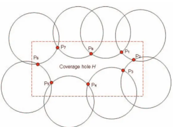
Figure 2. A demonstration of diameter calculation. The diameter of coverage hole H equals to the maximum Euclidean distance between the intersection points a and b in point set ΩHm, i.e., d(H) =
maxa,b∈ΩHmdist(a, b), herebyΩHm = {P1, P2,· · ·, P8}is the set of intersection points on the boundary holeH.
The theorem above is first presented and proved in [14]. Considering the sensing region of a sensor is open disc, the problem of region coverage can be easily transformed into the problem of finding a vertex cover [13].
Recall that the diameter of a coverage hole is defined as the largest Euclidean distance between any two points in the coverage hole. Let Ωa denote the set of intersection points of all active sensors’ sensing boundaries. Without loss of generality, we also consider the situation on the edge of A by adding intersection points among all active sensors’ sensing boundaries and the boundary ofAinto setΩa. The set ΩHm denotes the intersection points on the border of
Hm.
Secondly, the diameter of coverage hole Hm equals to
d(ΩHm)if the sensing regions are convex, i.e.,
d(Hm) =d(ΩHm) = maxa,b∈Ω
Hmdist(a, b),
(6)
where d(ΩHm)denotes the largest Euclidean distance
be-tween any two points in setΩHm.
The theorem above and detailed proof are first pre-sented in [10]. We can therefore calculate the diameter of a coverage hole in a convenient way. An example is demonstrated in Fig. 2. In Fig. 2, the boundary of coverage hole H is composed of sensors’ sensing boundaries and
ΩHm = {P1,· · ·, P8}, are the intersection points of these
sensing borders. The diameter of coverage holeH equals to the maximum Euclidean distance of the intersection points inΩHm, i.e.,d(H) = maxa,b∈ΩHmdist(a, b).
B. Trap Cover Optimization
If D = 0, Minimum Weight Trap Cover Problem boils down to a set covering problem which has already been proved to be NP-hard [25]. Therefore, Minimum Weight Trap Cover Problem is NP-hard which can not be solved in polynomial time unlessP =N P.
In this section, we discuss how to find aminimum weight trap coverin detail. We develop an efficient approximation algorithm Trap Cover Optimization (TCO) to solve mini-mum weight trap cover problem. AssumeCis theminimum
weight sensor cover[11] which provides full coverage toA andCis the trap cover obtained by TCO. We will deriveC from setC in TCO, i.e.,C⊆C.
TCO is composed of two major steps. Firstly, aminimum weight sensor coverC is selected to cover the whole RoI A, which is viewed as Minimum Weight Sensor Cover Problem [11]. We regard all intersection points in Ω as targets to be covered. Existing literatures have developed algorithms to efficiently solve this problem [4], [13], [26]. Secondly, we remove sensors in C successively until C is empty. We let Ψrepresent C∪C for simplicity in our description. A sensoriis added to set C if it satisfies that the maximum coverage hole diameter of (Ψ−i) exceeds the thresholdD, which means it is not removed from setΨ. The sensors which are not removed fromΨare all retained inC ultimately. Our aim is to remove as many sensors with poor residual energy fromΨas possible so that the output of TCO,Ccontains only a few sensors and they are rich in residual energy. We will discuss next how to remove sensors in a proper order to achieve better performance.
In Algorithm 1, we let DΨ(i) represent the aggregate
diameters of all coverage holes which are covered by sensor i but not covered by set (Ψ−i), i.e., the sum of diameters of all newly emerging coverage hole when sensoriis removed, which is the largest possible increment of a coverage hole. Let ΩΨ(i) represent all intersection points which are covered by setC but not covered by set
(Ψ−i). Assume points in set ΩΨ(i) belong to boundary points ofMicoverage holes. Accordingly, we divideΩΨ(i)
intoΩΨ1(i),ΩΨ2(i),· · ·,ΩΨMi(i). Assume the diameters of
these coverage holes aredΨ1(i),· · ·, dΨMi(i), respectively.
We set DΨ(i) = min{ Mi j=1 dΨj(i),2r} (7)
which means that DΨ(i) should not be greater than the
diameter of sensing region of a sensor, since the diam-eter of sensing region restricts the largest increment of a coverage hole when sensor i is removed. Essentially, DΨ(i)is supposed to be the upper bound of increment of a
coverage hole’s diameter when sensor i is removed from C. We argue that DΨ(i) is an important factor because
it depicts the possible effect of a candidate sensor on the diameter of existing coverage holes. SinceDΨ(i)restrains
the increment of coverage hole’s diameter when sensor i is removed from C, we can safely remove sensors with low DΨ(i) whose effects on the existing coverage holes
are bounded. Thus, more sensors can be removed before the diameter of any coverage hole is beyondD. We adoptDΨ(i)
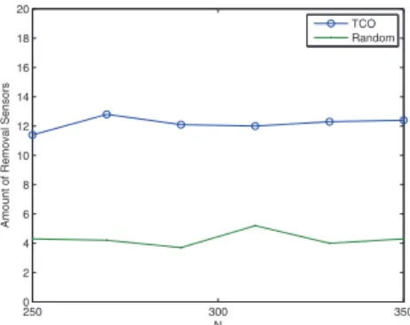
in TCO as an important factor. We also conduct simulation experiments to justify our design. Sensors with same weights are deployed randomly and a full cover setCis picked with aforementioned methods. We compare the amount of sensors removed from Ψ between TCO and a random approach
250 300 350 0 2 4 6 8 10 12 14 16 18 20 N
Amount of Removal Sensors
TCO Random
Figure 3. Amount of removed sensors by TCO and random approach vs.
N,D= 25
which randomly selects a sensor to remove. The average results are plotted in Fig. 3, which shows that TCO improves the amount of removed sensors significantly by considering DΨ(i).
We consider to normalize the weights of sensors byDΨ(i)
to determine which sensor is to be removed. DΨ(i) is a
variable between 0 and2r. To avoid zero in denominator,we set the normalized factor as 1/(1 +αDΨ(i)), where α =
1/(2r). Furthermore, the normalized weightG(i)of sensor i is defined, i.e., G(i) = wi/(1 +αDΨ(i)). We remove the sensor with the greatest normalized weightG(i) each time. In this way, sensors with less residual energy or greater upper bound of increment of a coverage hole, i.e.,DΨ(i), are supposed to be removed fromΨwith a higher priority. Every sensori in setC are checked iteratively and added to C if the maximum coverage hole diameter of(Ψ−i) exceeds the thresholdD, while the uncovered intersection points and coverage holes are updated accordingly. TCO terminates when C is empty. The remaining set C is the output of TCO.
Sensors with no residual energy are not involved in minimum weight sensor cover C since they have infinite weights, unless there are no set covers with residual energy to provide full coverage. Even if sensors with no residual energy are involved in C, they are removed first in TCO because they have infinite normalized weights. If the output of TCO, C contains sensors with no residual energy, it indicates that there are no trap covers with redundant energy to provideD-trap coverage any more, which means that the network reaches the end of its lifetime.
We useG(i)as an important guidance to remove sensors but it is not always the best especially when removing a sensoriwith highG(i)will cause violation against restraint ofD, which may force the algorithm to return a trap cover instantly. We try to tackle with the problem in our algorithm. In TCO, we enumerate every candidate sensorisuccessively according to the magnitude of itsG(i). A sensor is removed fromΨ only if it will not cause violation against restraint ofD. In this way, we can ensure that the restraint ofDwill not be exceeded prematurely.
The detailed algorithm is shown in Algorithm 1 andd(Ψ) is used to represent the maximum diameter of coverage holes
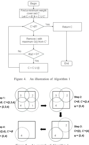
Figure 4. An illustration of Algorithm 1
Figure 5. An example of Algorithm 1
when only sensors in setΨare activated. We also illustrate TCO in Fig. 4.
Algorithm 1Trap Cover Optimization
1) Find aminimum weight cover set C using Greedy-MSC in [4] which ensures the whole region A is covered. Let C = ∅,α = 1/(2r). Let Ψ represent C∪C.
2) For every sensor i in set C, calculate G(i) = wi/(1 +αDΨ(i)). IfC=∅, return trap coverC.
3) Find the sensori with maximum G(i)and remove ifromC.
4) Update existing uncovered intersection points in A and the boundaries of coverage holes with respect to setΨ.
5) Calculated(Ψ). Ifd(Ψ)> D, then letC=C∪{i}. 6) Back to step 2.
Consider a simple example in Fig. 5. The four sensors in set C are deployed symmetrically which full cover the square region with side lengthaand setCis empty initially. The sensors are assumed to have the same weights. The threshold of coverage hole is supposed to be less than a. We will show how TCO works then. At first, we assume
TCO picks Sensor 1 to be removed from setC. Sinced(Ψ) whereΨ =C∪C is not beyond the threshold, Sensor 1 will not be added into set C. Next, we find that Sensor 3 has the lowestDΨ(i)amongCandΨonly contains Sensor
2,3,4 now. Considering the sensors have the same weights, we will remove Sensor 3 fromC. After that,d(Ψ)is still not beyond the threshold, so Sensor 3 will not be added into set C either. We then remove Sensor 2 from set C. The diameter of Ψ which only contains Sensor 4 can not provide required trap coverage any more, so we add Sensor 2 into setC. In the same way, we remove Sensor 4 from C and add it into setC. Finally, TCO terminates whenC is empty and Sensor 2 and 4 inC are activated to provide required trap coverage.
The time complexity of TCO is apparently polynomial since we only enumerate the elements inConce. Later on, we will prove the approximation ratio of TCO is only related to the sensor deployment density in Section V. Simulations in Section VI have confirmed thatG(i)based TCO always picks trap cover with higher average residual energy and lower energy consumption.
V. PERFORMANCEANALYSIS
A. Theoretical Analysis
We investigate the performance of our proposed algorithm TCO theoretically in this section.
Before the derivation, we make assumptions as follows.
Assumption 1: Given RoI Aof sizel1×l2,l1r+D
andl2r+D, whereris the sensing range of each sensor
andDis the diameter threshold ofD-trap coverage. We will first prove the ratio bound of aggregate weight between the outputC and the initial input C of TCO. Let NC denote the number of sensors inC.
Lemma 1: wC≤ 2NC2+ND/C(2r)wC.
Proof:LetC=C−Cdenote the set of sensors which are removed from setCby Algorithm 1. Here we useD(i) to representDΨ(i)for simplicity. Suppose at the(k+ 1)th
iteration d(Ck+1) exceeds threshold D for the first time. LetQ denote the set C−Ck, where Ck is C at the kth
iteration. Thus,C ⊆Ck. Obviously,Q⊆C, which means wQ≤wC.
Since TCO always selects to remove sensor i from C with maximumG(i) =wi/(1 +αD(i)), we get that,
wQ i∈Q(1+αD(i)) ≥maxj∈C{1+αDwj(j)} ≥ wC j∈C(1+αD(j)) (8) According to the definition of set Q and D(i), the upper bound of the incremental of maximum coverage hole diameter, we have
i∈Q
D(i)≥D−2r (9) With Eq.(8), (9) andα= 1/(2r),
wC wC ≥ wQ wC ≥ i∈Q(1+αD(i)) j∈C(1+αD(j)) ≥ αD (1+2αr)NC (10)
With the Eq. wC=wC+wC, we have wC wC ≤ (1 + 2αr)NC (1 + 2αr)NC+αD (11) wC≤ 2 2NC NC+D/(2r)wC (12)
where concludes the proof.
We denote the optimum minimum weight trap cover which provide D-trap coverage as OP T. Let N1 denote the number of sensors inOP T.
Lemma 2: The number of sensors providingD-trap cov-erageto RoIAof sizel1×l2must be greater than 3√3(2rS+D)2
whereS=l1×l2.
Proof: As referred in [10], if the sensing radius r is increased to(r+D), the sensor set will provide full coverage toA.
Figure 6. Optimal deployment on the vertices of equilateral triangles It is well-known that it is optimal to deploy sensor nodes of disk sensing model on the vertices of equilateral triangles to cover a plane [27]. If l1r+D andl2r+D,
ac-cording to the property of equilateral triangles, the minimum number of sensors with sensing ranger+Dwhich provide full coverage to the RoIAis 3√ 2S
3(r+D)2. We have
N1≥ 2S
3√3(r+D)2. (13)
This concludes the proof.
Assume that wOP T denotes the aggregate weight of
sensors in setOP T. According to equation (3), the weight of energy-redundant sensori,w(i)satisfies thatθ/E > w(i)≥
1/E. We have wOP T ≥N1/E. (14) wC wOP T < Nθ/E N1/E ≤θN3 √ 3(r+D)2 2S =ρθ3 √ 3(r+D)2 2 . (15)
We have the following main result for TCO, which theoretically guarantees the performance of TCO even in the worst case. Based on Lemma.1, we have the following theorem,
Theorem 1: wC/wOP T < 2NC2+ND/C(2r)ρθΦ, whereΦ =
3√3(r+D)2
2 .
Asθ,r andDare constants, the approximation ratio of TCO is only related to the density ρ. As the number of sensors in a full cover setNC increases, the approximation ratio approachesρθΦ, which is treated asO(ρ). The bound guarantees the approximation ratio of TCO compared with optimal solution even in the worst case. If more and more sensor nodes are placed, the optimal solution improves quickly since more options are available. Compared with optimal solution, our algorithm relatively improves slower. Thus, the worst bound may deteriorate asρincreases.
B. Simulation Performance
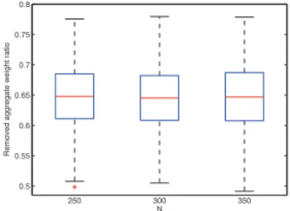
We conduct simulations to validate the performance of TCO. The ratio of the aggregate weight of removed sensors to the aggregate weight of initial full cover sensor set is viewed as the indicator of the performance of TCO. We present the boxplot in Fig. 7, which shows the statistics of running for 300 times to test the performance of TCO in average. As we can see, TCO performs well both in the average case and in the worst case. The removed aggregate weight ratio is even above 0.45 in the worst case, which guarantees the effect of employing TCO.
0.5 0.55 0.6 0.65 0.7 0.75 0.8 250 300 350 N
Removed aggregate weight ratio
Figure 7. Removed aggregate weight ratio vs.N,D= 40
0 5 10 15 20 25
0 20 40
Removed sensors
Maximum hole diameter
0 5 10 15 20 250
5
Aggregate weight
Figure 8. Status of maximum hole diameter and aggregate weight during TCO running,D= 40
We also record the status of maximum hole diameter and aggregate weight of sensors in Ψduring a period of TCO
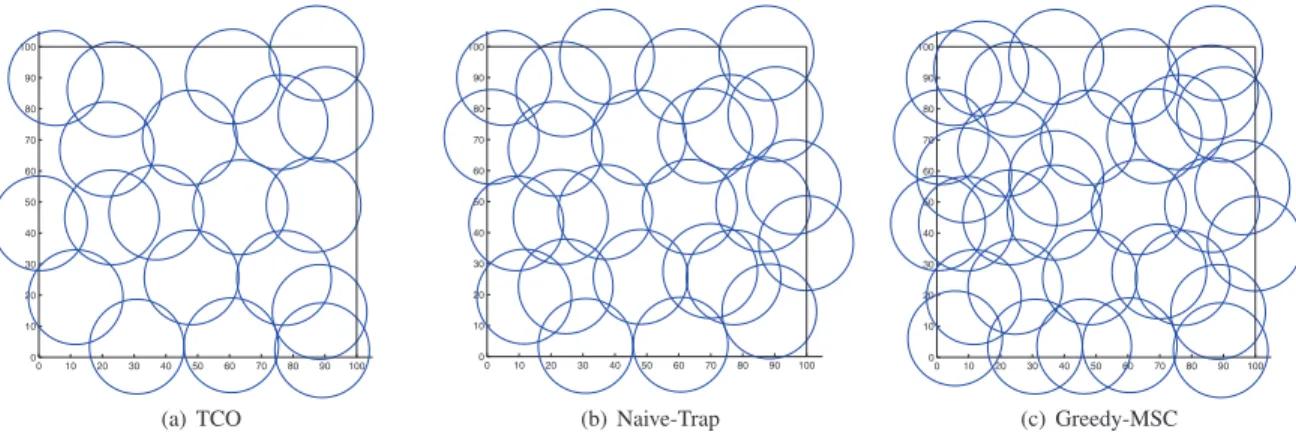
0 10 20 30 40 50 60 70 80 90 100 0 10 20 30 40 50 60 70 80 90 100 (a) TCO 0 10 20 30 40 50 60 70 80 90 100 0 10 20 30 40 50 60 70 80 90 100 (b) Naive-Trap 0 10 20 30 40 50 60 70 80 90 100 0 10 20 30 40 50 60 70 80 90 100 (c) Greedy-MSC
Figure 9. Coverage during a time slot of Naive-Trap, TCO and Greedy-MSC Heuristic in RoI.N= 300,E= 20,D= 25. Blue circles denote the sensing region of activated sensors.
running in Fig. 8. The results illustrate the running status of TCO. The maximum hole diameter increases very slowly when it approachesD. That is because we remove sensors not just depend onG(i). We enumerate each candidate sen-sorisuccessively according to the magnitude ofG(i)when the maximum hole diameter is about to exceedD. Candidate sensoriis removed only if it will not cause violation against restraint of D. Hence, many sensors are removed with no significant effect on maximum hole diameter at the end.
VI. SIMULATIONRESULTS
A. Experiment Setup
The WSN in our simulations has N sensors, each with an initial energy ofE units and a sensing range of 15 units. The sensors are deployed randomly in a square of100×100 units2. Active sensors in each time slot consume 1 unit of energy. We assume that the switching frequency is very low so that the costs including residual energy information collection and scheduling information dissemination are negligible in the simulations. The diameter threshold of trap coverage isDunits.
The simulations are conducted mainly in following pro-cedures. Firstly, at the beginning of each time slot, each sensor is assigned with a weight according to its residual energy. The sensor with more residual energy is assigned lower weight. Secondly, we employ specified algorithm to find a D-trap cover and only sensors in the trap cover are activated during each time slot. Finally, the lifetime of network terminates if there exist no trap covers with redundant energy to provideD-trap coverage any more.
B. Energy balance and consumption
In this section, we conduct extensive simulations to eval-uate the performance of TCO in a lifetime span of WSN.
The best algorithm to the maximum network lifetime under full coverage model, to our best knowledge, is Greedy-MSC Heuristic [4]. We describe a naive approach used in the simulation to compare with TCO. We name the naive approach as Naive-Trap, which is slightly modified from the Greedy-MSC Heuristic algorithm with adjustment to the
trap coverage requirement. AssumeU(k) =z(k)/wk for a sensorkwherez(k)is the number of uncovered intersection points covered by k and wk is the weight of sensor k. This algorithm always sets the sensor k∗ with maximum U(k∗)to be active iteratively until the region achievesD -trap coverage. At each time slot, sensors are assigned with weights and a minimum weight trap cover is activated by the naive approach until the network expires. Since no trap coverage based scheduling algorithm has been proposed before, Naive-Trap which guarantees D-trap coverage is considered to be the state-of-the-art solution.
0 50 100 150 200 0 10 20 30 40 50 60 70
Active amount of sensors
time
Greedy−MSC Naive−Trap TCO
Figure 10. Active amount of sensors vs. time slot,E= 20,D= 15,N= 300 0 100 200 300 400 500 0 10 20 30 40 50 60
Active amount of sensors
time
Greedy−MSC Naive−Trap TCO
Figure 11. Active amount of sensors vs. time slot,E= 30,D= 25,N= 400
Simulations are performed for these three algorithms under the same setting. We assign weights to sensors at the beginning of each time slot and treat each intersection point as a target inGreedy-MSC Heuristic. We compare trap
coverage with full coverage in the simulations because there is no existing work of conducting experiments to verify the significant improvement of energy consumption and lifetime under trap coverage in WSNs of large scale.
0 10 20 30 40 50 60 70 80 0 0.1 0.2 0.3 0.4 0.5 0.6 0.7 0.8 0.9 1
Residual energy ratio
time slot
Greedy−MSC Naive−Trap TCO
Figure 12. Average residual energy of activated sensors vs. time slot,
E= 10,D= 15,N= 300 0 50 100 150 200 250 300 0 0.1 0.2 0.3 0.4 0.5 0.6 0.7 0.8 0.9 1
Residual energy ratio
time slot
Greedy−MSC Naive−Trap TCO
Figure 13. Average residual energy ratio of activated sensors vs. time slot,
E= 20,D= 25,N= 400
Since we assume that inactive sensors do not consume any energy, the number of active sensors per time slot denotes the energy consumption. We conduct simulations to compare the active number of sensors during the lifetime running by these three algorithms. The results in Fig. 10 and Fig. 11 suggest that the energy consumption of our algorithm is the lowest, which may lead to a longer lifetime. In order to balance the energy consumption of sensors, sensors with more residual energy are activated with higher priority. Results in Fig. 12 and Fig. 13 show the average residual energy of activated sensors by these three algorithms, which demonstrates that TCO always activates sensors with higher residual energy. We also illustrate the coverage of these three algorithms during a time slot in Fig. 14, where blue circles denotes the sensing region of activated sensors. Our algorithm apparently activates less sensors to provide required quality of trap coverage compared with Naive-Trap andGreedy-MSC Heuristic according to Fig. 14. We can learn that trap coverage model is an energy-efficient model since its energy consumption per slot is only half of that of full coverage model while the diameter of coverage hole is constrained to be below the diameter of sensor’s sensing region, which might be acceptable in many cases. We have three observations about the results. Firstly, Naive-Trap always picks up active sensors without backtracking,
while TCO finds a minimum weight sensor cover at the beginning and then removes the redundant sensors, which means TCO determines active sensor set globally and thus more efficiently. Secondly, TCO considers the effect of each sensor on the diameter of coverage hole directly.DΨ(i)of
sensorias the upper bound of increment of coverage hole’s diameter is taken into consideration, which can significantly reduce the amount of activated sensors. The importance of DΨ(i) is validated in Fig. 3. We define G(i) as the
normalized weight in TCO to tradeoff between upper bounds of increment and weights of sensors, and remove sensors from initial sensor set based on G(i). Thirdly, instead of ending the algorithm prematurely, we enumerate all sensors to check whether we can remove more sensors when the diameter of coverage hole is about to exceedD. Trap cover with lower energy consumption and higher residual energy can always be obtained by TCO. Therefore, our algorithm outperforms Naive-Trap.
C. Lifetime performance evaluation
The lifetimes achieved by Naive-Trap,TCOand Greedy-MSC Heuristic versus different scenarios are plotted in Fig. 14(a) and Fig. 14(b). The lifetime is lengthened if the number of deployed sensorsN or the initial energy of each sensorE increases. The plots suggest thatTCOalways has a better performance of longevity compared with Naive-Trap in different scenarios. That is because TCO always has lower energy consumption and activates sensors with higher residual energy, which is shown in aforementioned plots. The simulation results also prove that trap coverage can extend the network lifetime significantly. We vary the diameter threshold D to compare the lifetimes achieved by Naive-Trap and TCO and Greedy-MSC Heuristic in Fig. 14(c). The network lifetime increases if we allow a larger D. Since Greedy-MSC Heuristic has nothing to do with the diameterD, the lifetime remains unchanged when Dvaries.
VII. DISCUSSION ANDCONCLUSION
In this paper, we have investigated the problem of trap coverage in WSNs. Minimum Weight Trap Cover Problem
is formulated to schedule the activation of sensors in WSNs under the model of trap coverage. We always activate the minimum weight trap cover successively at each time slot to balance the energy consumption of each sensor so that the longevity of networks is ensured. A novel algorithm is proposed to tackle with the problem based on trap coverage which is shown in simulation results to have better performance than a naive approach. The performance of Minimum Weight Trap Coverage we find is proved to be at most O(ρ)times of the optimal solution, where ρ is the density of sensor nodes in the region.
Our algorithm, as a centralized algorithm, outperforms
consump-250 300 350 400 20 30 40 50 60 70 80 90 100 lifetime Number of sensors, N Greedy−MSC Naive−Trap TC−NLO (a) Lifetimes vs.N,E= 10,D= 15 10 15 20 25 30 35 40 0 50 100 150 200 250 300 lifetime
Initial energy of each sensor, E Greedy−MSC Naive−Trap TC−NLO (b) Lifetimes vs.E,N= 300,D= 15 15 20 25 30 35 0 50 100 150 200 250 300 lifetime
Threshold of hole diameter, D Greedy−MSC
Naive−Trap TC−NLO
(c) Lifetimes vs.D,N= 300,E= 20
Figure 14. Lifetimes of Naive-Trap, TCO and Greedy-MSC Heuristic
tion and lifetime. Naive-Trap is centralized while Greedy-MSC Heuristiccan be designed ad hoc. Thus,Greedy-MSC Heuristicis relatively easy to deploy and may need less extra communications during operation. In fact, it is a hard task to design a distributed scheduling scheme to achieve trap coverage because the diameter of coverage hole is always larger than a sensor’s sensing range and communication range. Hence, it is rather difficult for sensors to guarantee the size of a coverage hole in a distributed way.
VIII. ACKNOWLEDGEMENTS
This work was supported in part by the Natural Science Foundation of China (NSFC) under Grants 61004060 and 60974122, Joint Funds of NSFC-Guangdong under Grant U0735003, the Natural Science Foundation of Zhejiang Province under Grant R1100324, SUTD-ZJU Collaboration Grant SUTDZJU/ RES/03/2011 and the 111 Projects under Grant B07031.
REFERENCES
[1] J. Ko, C. Lu, M. Srivastava, J. Stankovic, A. Terzis, and M. Welsh. Wireless sensor networks for healthcare. Pro-ceedings of IEEE, 2010.
[2] S. Zahedi, M. Srivastava, C. Bisdikian, and L. Kaplan. Quality tradeoffs in object tracking with duty-cycled sensor networks. InRTSS, 2010.
[3] Y. Liu and W. Liang. Approximate coverage in wireless sensor networks. InIEEE LCN, 2005.
[4] M. Cardei, T. Thai, Y. Li, and W. Wu. Energy-efficient target coverage in wireless sensor networks. InIEEE INFOCOM, 2005.
[5] S. Slijepcevic and M. Potkonjak. Power efficient organization of wireless sensor networks. InIEEE ICC, 2001.
[6] S. He, J. Chen, D. Yau, H. Shao, and Y. Sun. Energy-efficient capture of stochastic events by global- and local-periodic network coverage. InACM MobiHoc, 2009. [7] J. Jeong, Y. Gu, T. He, and D. Du. VISA: Virtual Scanning
Algorithm for Dynamic Protection of Road Networks. In
IEEE INFOCOM, 2009.
[8] G. Wang, G. Cao, and T. Porta. Movement-assisted sensor deployment. InIEEE INFOCOM, 2004.
[9] B. Liu and D. Towsley. A study of the coverage of large-scale sensor networks. InIEEE MASS, 2004.
[10] P. Balister, Z. Zheng, S. Kumar, and P. Sinha. Trap coverage: Allowing coverage holes of bounded diameter in wireless sensor networks. InIEEE INFOCOM, 2009.
[11] P. Berman, G. Calinescu, C. Shah, and A. Zelikovsky. Effi-cient energy management in sensor networks. Ad Hoc and Sensor Network, Wireless Networks, 2005.
[12] S. Meguerdichian, F. Koushanfar, M. Potkonjak, and M. Sri-vastava. Coverage problems in wireless ad-hoc sensor net-works. InIEEE INFOCOM, 2001.
[13] S. Yang, F. Dai, M. Cardei, and J. Wu. On multiple point coverage in wireless sensor networks. InIEEE MASS, 2005. [14] G. Kasbekar, Y. Bejerano, and S. Sarkar. Lifetime and cov-erage guarantees through distributed coordinate-free sensor activation. InACM MobiCom, 2009.
[15] D. Dong, Y. Liu, K. Liu, and X. Liao. Distributed coverage in wireless ad hoc and sensor networks by topological graph approaches. InIEEE ICDCS, 2010.
[16] S. Ren, Q. Li, H. Wang, X. Chen, and X. Zhang. Design and analysis of sensing scheduling algorithms under partial coverage for object detection in sensor networks.IEEE Trans. on Parallel and Distributed Systems, 18, 2007.
[17] R. Balasubramanian, S. Ramasubramanian, and A. Efrat. Coverage time characteristics in sensor networks. In IEEE MASS, 2006.
[18] S. Sankararaman, A. Efrat, S. Ramasubramanian, and J. Taheri. Scheduling sensors for guaranteed sparse coverage.
http://arxiv.org, 2009.
[19] C. Gui and P. Mohapatra. Power conservation and quality of surveillance in target tracking sensor networks. In ACM MobiCom, 2004.
[20] Q. Cao, T. Abdelzaher, T. He, and J. Stankovic. Towards optimal sleep scheduling in sensor networks for rare-event detection. InACM/IEEE IPSN, 2005.
[21] P. Balister and S. Kumar. Random vs. deterministic deploy-ment of sensors in the presence of failures and placedeploy-ment errors. InIEEE INFOCOM, 2009.
[22] J. Hwang, T. He, and Y. Kim. Exploring in-situ sensing irregularity in wireless sensor networks. In ACM SenSys, 2007.
[23] T. Yan, Y. Gu, T. He, and J. Stankovic. Design and opti-mization of distributed sensing coverage in wireless sensor networks. IEEE Trans. on Embedded Computing System. [24] X. Wang, G. Xing, Y. Zhang, C. Lu, R. Pless, and C. Gill.
Integrated coverage and connectivity configuration in wireless sensor networks. InACM SenSys, 2003.
[25] Richard M. Karp. Reducibility among combinatorial prob-lems. In50 Years of Integer Programming 1958-2008, pages 219–241. Springer Berlin Heidelberg, 2010.
[26] M. Cardei and D. Du. Improving wireless sensor network life-time through power aware organization. Wireless Networks, 2005.
[27] X. Bai, S. Kumar, D. Xuan, Z. Yun, and T. Lai. Deploying wireless sensors to achieve both coverage and connectivity. InACM MobiHoc, 2006.