Lecture Notes on Liveness Analysis

Liveness Analysis

Lecture 4 September 4, 2014

1

Introduction

We will see different kinds of program analyses in the course, most of them for the purpose of program optimization. The first one, liveness analysis, is required for register allocation. A variable isliveat a given program point if it will be used during the remainder of the computation, starting at this point. We use this infor-mation to decide if two variables could safely be mapped to the same register, as detailed in the last lecture.

Is liveness decidable? Like many other properties of programs, liveness is un-decidable if the language we are analyzing is Turing-complete. The approximation we describe here is standard, although its presentation is not. Chapter 10 of the textbook [App98] has a classical presentation.

2

Liveness by Backward Propagation

Consider a 3-address instruction applying a binary operator⊕:

x ← y⊕z

There are two reasons a variable may be live at this instruction, by which we mean live just before the instruction is executed. The first is immediate: if a variable (here:

yandz) is used at an instruction, it is used in the computation starting from here. The second is slightly more subtle: since we execute the following instruction next, anything we determine is live at the next instruction is also live here. There is one exception to this second rule: because we assign to x, the value ofxcoming into this instruction does not matter (unless it is y or z), even if it is live at the next instruction. In summary,

1. yandzare live at an instructionx←y⊕z.

2. uis live atx←y⊕zifuis live at the next instruction andu6=x.

Similarly, for an instructionx←cwith a constantc, we find thatuis live at this instruction ifuis live at the next instruction andu6=x.

As a last example,x is live at a return instructionreturn x, and nothing else is live there.

If we have a straight-line program, it is easy to compute liveness information by going through the program backwards, starting from the return instruction at the end. In that case, it is also precise rather than an approximation. As an exam-ple, one can construct the set of live variables at each line in this simple program bottom-up, using the two rules above.

x             

Instructions Live-in Variables

x1 ← 1 · x2 ← x1+x1 x1 x3 ← x2+x1 x1, x2 y2 ← x1+x2 x1, x2, x3 y3 ← y2+x3 y2, x3 return y3 y3

For example, looking at the 4th line, we see thatx1 andx2 are live because of the

first rule (they are used) andx3is live because it is live at the next instructions and

different fromy2.

3

Liveness Analysis in Logical Form

Before we generalize to a more complex language of instructions, we try to specify the rules for liveness analysis in a symbolic form to make them more concise and to avoid any potential ambiguity. For this we give each instruction in a program a line number orlabel. If an instruction has labell, we writel+ 1for the label of the next instruction.

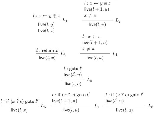
We also introduce the predicate live(l, x) which should be true when variable

x is live at linel. We then turn the rules stated informally in English into logical rules. l:x←y⊕z live(l, y) live(l, z) L1 l:x←y⊕z live(l+ 1, u) x6=u live(l, u) L2

Here, the formulas above the line are premises of the inference rule and the formulas below the line are the conclusions. If all premises are true, we know all conclusions must be true. To the right of the line we write the name of the inference rule. For example, we can read ruleL1 as: “If linelhas the formx ← y⊕zthenyis

live atlandzis live atl.”

This is somewhat more abstract than the backward propagation algorithm be-cause it does not specify in which order to apply these rules. We can now add more rules for different kinds of instructions.

l:returnx live(l, x) L3 l:x←c live(l+ 1, u) x6=u live(l, u) L4

If we only have binary operators, moves of constants into variables, and return instructions, then these four rules constitute a complete specification of when a variable should be live at any point in a program.1

This specification also gives rise to an immediate, yet somewhat nondeterminis-tic implementation. We start with a database of facts, consisting only of the original program, with each line properly labeled. Then we apply rules in an arbitrary or-der — whenever the premises are all in the database we add the conclusion to the database. Applying one rule may enable the application of another rule and so on, but eventually this process will not gain us any more information. At this point, we can still apply rules but all conclusions are already in the database of facts. We say that the database issaturated. Since the rules are a complete specification of our liveness analysis, by definition a variablexis deemed lived at linelif and only if the factlive(l, x)is in the saturated database.

This may seem like an unreasonably expensive way to compute liveness, but in fact it can be quite efficient, both in theory and practice.

In theory, we can look at the rules and determine their theoretical complexity by (a) counting so-calledprefix firingsof each rule, and (b) bounding the size of the completed database. We will return to prefix firings, a notion due to McAllester [McA02], in a later lecture. Bounding the size of the completed database is easy. We can infer at mostL·V distinct facts of the formlive(l, x), whereLis the number of lines andV

is the number of variables in the program. Counting prefix firings does not change anything here, and we get a theoretical complexity ofO(L·V)for the analysis so far.

In practice, there are a number of ways logical rules and saturation can be implementation efficiently. One uses Binary Decision Diagrams (BDD’s). Wha-ley, Avots, Carbin, and Lam [WACL05] have shown scalability of global program 1_{As pointed out in lecture, we should really also have a pure move instructionx←y. We leave it}

analyses using inference rules, transliterated into so-called Datalog programs. See Smaragdakis and Bravenboer’s work on Doop [SB10] for a different technique. Un-fortunately, there is no Datalog library that we can easily tie into our compilers, so while we specify and analyze the structure of our program analyses via the use of inference rules, we generally do not implement them in this manner. Instead, we use other implementations that follow the ideas that are identified precisely and concisely by the logical rules. Because our logical rules identify the fundamental principles, this presentation makes it easier to understand the important issues of liveness analysis. This also helps capturing the implementation-independent com-monality among different styles of implementation. We will see throughout this whole course, that logical rules can capture many other important concepts in a similarly simple way.

4

Loops and Conditionals

The nature of liveness analysis changes significantly when the language permits loops. This will also be the case for most other program analyses.

Here, we add two new forms of instructions, and unconditional jumpl:gotol0, and a conditional branchl:if(x?c)gotol0, where “?” is a relational operator such as equality or inequality.

We now discuss how liveness analysis should be extended for these two forms of instructions. A variableuis live atl:gotol0 if it is live atl0. We capture this with the following inference rule, which is the only rule pertaining togoto

l:gotol0

live(l0, u) live(l, u) L5

When executing a conditional branchl:if (x?c)gotol0 we have two potential successor instructions: we may go to the nextl+ 1if the condition is false or tol0

if the condition is true. In general, we will not be able to predict at compile time whether the condition will be true or false and usually it will sometimes be true and sometimes be false during the execution of the program. Therefore we have to consider a variable live atlif it is live at the possible successorl+ 1or it is live at the possible successorl0. Also, the instruction usesx, soxis live. Summarizing this as rules we obtain l:if (x?c)gotol0 live(l, x) L6 l:if(x?c)gotol0 live(l+ 1, u) live(l, u) L7 l:if (x?c)gotol0 live(l0, u) live(l, u) L8 These rules are straightforward enough, but if we have backwards branches we will not be able to analyze in a single backwards pass. As an example to

illus-trate this point, we will use a simple program for calculating the greatest common divisor of two positive integers. We assume that at the first statement labeled 1, variables x1 andx2 hold the input, and we are supposed to calculate and return

gcd(x1, x2). x                    Live variables, Instructions initially 1 : if (x2 = 0)goto8 2 : q←x1/x2 3 : t←q∗x2 4 : r←x1−t 5 : x1 ←x2 6 : x2 ←r 7 : goto1 8 : returnx1

If we start at line 8 we seex1is live there, but we can conclude nothing (yet) to

be live at line 7 because nothing is known to be live at line 1, the target of the jump. After one pass through the program, listing all variables we know to be live so far we arrive at: x                    Live variables, Instructions after pass 1 1 : if (x2 = 0)goto8 x1, x2 2 : q←x1/x2 x1, x2 3 : t←q∗x2 x1, x2, q 4 : r←x1−t x1, x2, t 5 : x1 ←x2 x2, r 6 : x2 ←r r 7 : goto1 · 8 : returnx1 x1

At this point, we can apply the rule forgototo line 7, once with variablex1and

once withx2, both of which are now known to be live at line 1. We list the variables

that are now further to the right, and make another pass through the program, applying more rules.

x                    Live-in variables,

Instructions after pass 1 after pass 2 saturate 1 : if(x2 = 0)goto8 x1, x2 2 : q←x1/x2 x1, x2 3 : t←q∗x2 x1, x2, q 4 : r←x1−t x1, x2, t 5 : x1 ←x2 x2, r 6 : x2 ←r r x1 7 : goto1 · x1, x2(from1) 8 : returnx1 x1

At this point our rules have saturated and we have identified all the live vari-ables at all program points. From this we can now build the interference graph and from that proceed with register allocation.

The algorithm which saturates the inference rules implies that a variable is des-ignated live at a given line only if we have definitive reason to believe it might be live. Consider the program

1 : u1←1

2 : y ←y∗x

3 : z←y+y (znot used, redundant) 4 : x←x−u1

5 : if (x >0)goto2 6 : returny

which has a redundant assignment to zin line 3. Sincez is never used, z is not found to be live anywhere in this program. Nevertheless, unless we eliminate line 3 altogether, we have to be careful to note thatzinterferes withx,u1, andybecause

those variables are live on line 4. If not,zmight be assigned the same register asx,

y, oru1and the assignment tozwould overwrite one of their values.

In the slightly different program 1 : u1←1

2 : y ←y∗x

3 : z←z+z (zlive but never needed) 4 : x←x−u1

5 : if (x >0)goto2 6 : returny

the variablezwill actually be inferred to be live at lines 1 through 5. This is because it is used at line 3, although the resulting value is eventually ignored. To capture redundancy of this kind is the goal ofdead code eliminationwhich requiresneededness analysisrather than liveness analysis. We will present this in a later lecture.

5

Refactoring Liveness

Figure1has a summary of the rules specifying liveness analysis.

l:x←y⊕z live(l, y) live(l, z) L1 l:x←y⊕z live(l+ 1, u) x6=u live(l, u) L2 l:returnx live(l, x) L3 l:x←c live(l+ 1, u) x6=u live(l, u) L4 l:gotol0 live(l0, u) live(l, u) L5 l:if (x?c)gotol0 live(l, x) L6 l:if(x?c)gotol0 live(l+ 1, u) live(l, u) L7 l:if (x?c)gotol0 live(l0, u) live(l, u) L8

Figure 1: Summary: Rules specifying liveness analysis (non-refactored) This style of specification is precise and implementable, but it is rather repet-itive. For example,L2 andL4 are similar rules, propagating liveness information

froml+ 1tol, andL1,L3andL6are similar rules recording the usage of a variable.

If we had specified liveness procedurally, we would try to abstract common pat-terns by creating new auxiliary procedures. But what is the analogue of this kind of restructuring when we look at specifications via inference rules? The idea is to identify common concepts and distill them into new predicates, thereby abstract-ing away from the individual forms of instructions.

Here, we arrive at three new predicates. 1. use(l, x): the instruction atlusesvariablex.

2. def(l, x): the instruction atldefines(that is, writes to) variablex. 3. succ(l, l0): the instruction executed afterlmay bel0.

Now we split the set of rules into two. The first set analyzes the program and generates the use, def and succ facts. We run this first set of rules to saturation.

Afterwards, the second set of rules employs these predicates to derive facts about liveness. It does not refer to the program instructions directly—we have abstracted away from them.

We write the second program first. It translates the following two, informally stated rules into logical language:

1. If a variable is used atlit is live atl.

2. If a variable is live at a possible next instruction and it is not defined at the current instruction, then it is live at the current instruction.

use(l, x) live(l, x) K1 live(l0, u) succ(l, l0) ¬def(l, u) live(l, u) K2

Here, we use¬to stand for negation, which is an operator that deserves more at-tention when using saturation via logic rules. For this to be well-defined we need to know thatdefdoes not depend onlive. Any implementation must first saturate the facts aboutdefbefore applying any rules concerning liveness, because the absence of a fact of the formdef(l,−)does not imply that such a fact might not be discov-ered in a future inference—unless we first saturate thedef predicate. Here, we can easily first apply all rules that could possibly conclude facts of the form def(l, u) exhaustively until saturation. If, after saturation with those rules (J1. . . J5below),

def(l, u)has not been concluded, then we know¬def(l, u), because we have exhaus-tively applied all rules that could ever conclude it. Thus, after having saturated all rules fordef(l, u), we can saturate all rules forlive(l, u). This simple saturation in stages would break down if there were a rule concludingdef(l, u)that depends on a premise of the formlive(l0, v), which is not the case.

We return to the first set of rules. It must examine each instruction and extract theuse,def, andsuccpredicates. We could write several subsets of rules: one subset to generate def, one to generateuse, etc. Instead, we have just one rule for each instruction with multiple conclusions for all required predicates.

l:x←y⊕z def(l, x) use(l, y) use(l, z) succ(l, l+ 1) J1 l:returnx use(l, x) J2 l:x←c def(l, x) succ(l, l+ 1) J3 l:gotol0 succ(l, l0) J4 l:if (x?c)gotol0 use(l, x) succ(l, l0) succ(l, l+ 1) J5

It is easy to see that even with any number of new instructions, this specification can be extended modularly. The main definition of liveness analysis in rules K1

andK2will remain unchanged and captures the essence of liveness analysis.

The theoretical complexity does not change, because the size of the database after each phase is still O(L·V). The only point to observe is that even though the successor relation looks to be bounded byO(L·L), there can be at most two successors to any linelso it is onlyO(L).

6

Implementing Liveness by Line or by Variable

When we implement the analysis, in the absence of a saturating datalog engine, we have to decide how to compute the information on the given program directly.

One option is to use sets of live variables associated with each line of the pro-gram. We start with the empty set everywhere and then walk backward along the control flow edges (from l0 to l if succ(l, l0)) computing the current approxi-mation to the live-in set for linel from the live-in set for linel0 and the variables defined at l. We must take care that if a line has multiple predecessors, we ex-plore all the alternatives. We stop on any particular branch when the new live set computed for a line is equal to the one already stored there. We refer to this as a line-oriented traversal, which we used earlier when we walked through an exam-ple. The line-oriented traversal has the disadvantage of potentially redundant set operations when loops are traversed multiple times.

Alternatively, we can perform a variable-oriented traversal. When we arrive at a line and see which variables are used there. For each such variable, we see if it is already live, in which case we do nothing. If it is not live, we declare it so and then walk backwards along the control flow edges propagating only the information for the single variable, stopping if it is already known to be live when we reach a line, or if it is defined at that line. This strategy actually achieves theO(L·V) bound, because for each variable we traverse at mostO(L)lines.

Here is how this would work in our example x                  Instructions 1 : if(x2 = 0)goto8 2 : q←x1/x2 3 : t←q∗x2 4 : r←x1−t 5 : x1 ←x2 6 : x2 ←r 7 : goto1 8 : returnx1

We start at line 8 and propagate the liveness ofx1to lines 1, 7, 6, in this order. We

in the column labeled (8). Line 7 does not use any variables, line 6 usesr which propagates only to line 5 (see column (6)). Line 5 usesx2which propagates around

the loop, etc. At the end, all variables used by lines 1 and 2 are already known to be live, so no further propagation takes place.

x                  Instructions (8) (6) (5) (4) (4) (3) 1 : if(x2 = 0)goto8 x1 x2 2 : q←x1/x2 x2 x1 3 : t←q∗x2 x2 x1 q 4 : r←x1−t x2 x1 t 5 : x1 ←x2 r x2 6 : x2 ←r x1 r 7 : goto1 x1 x2 8 : returnx1 x1

7

Control Flow

Properties of the control flow of a program are embodied in thesuccrelation intro-duced in the previous section. Thecontrol flow graphis the graph whose vertices are the lines of the program and with an edge betweenlandl0wheneversucc(l, l0). It captures the possible flows of control without regard to the actual values that are passed.

The textbook [App98] recommends an explicit representation of the control flow graph, together with the use ofbasic blocksto speed up analysis. Abasic block is a simple fragment of straight-line code that is always entered at the beginning and exited at the end. That is

• the first statement may have a label,

• the last statement terminates the control flow of the current block (with a goto, conditional branch, or a return), and

• all other statements in between have no labels (entry points) and no gotos or conditional branches (exit points).

From a logical perspective, basic blocks do not change anything, because they just accumulate a series of simple statements into one compound code block. Hence, it is not clear if a logical approach to liveness and other program analyses would actually benefit from basic block representations. But depending on the actual implementation technique, basic blocks can help surprisingly much, because the number of nodes that need to be considered in each analysis is reduced somewhat. Basic blocks basically remove trivial control flow edges and assimilate them into a

single basic block, exposing only more nontrivial control flow edges. Basic blocks are an example of an engineering decision that looks like a no-op, but can still pay off. They are also quite useful for SSA intermediate language representations and LLVM code generation.

Control flow information can be made more precise if we analyze the possible values that variables may take. Since control flow critically influences other anal-yses in a similar way to liveness analysis, it is almost universally important. Our current analysis is not sensitive to the actual values of variables. Even if we write

l : x←0

l+ 1 : if (x <0)gotol+ 3

l+ 2 : returny

l+ 3 : returnz (unreachable in this program due to values) we deduce that both y andz may be live at l+ 1even though onlyreturn y can actually be reached. This and similar patterns may seem unlikely, but in fact they arise in practice in at least two ways: as a result of other optimizations and during array bounds checking. We may address this issue in a later lecture.

8

Summary

Liveness analysis is a necessary component of register allocation. It can be specified in two logical rules which depend on the control flow graph,succ(l, l0), as well as information about the variables used,use(l, x), and defined,def(l, x), at each pro-gram point. These rules can be run to saturation in an arbitrary order to discover all live variables. On straight-line programs, liveness analysis can be implemented in a single backwards pass, on programs with jumps and conditional branches some iteration is required until no further facts about liveness remain to be discovered. Liveness analysis is an example of a backward dataflow analysis; we will see more analyses with similar styles of specifications throughout the course.

Questions

1. Can liveness analysis be faster if we execute it out of order, i.e., not strictly backwards?

2. Is there a program where liveness analysis gives imperfect information? 3. Is there a class of programs where this does not happen? What is the biggest

References

[App98] Andrew W. Appel. Modern Compiler Implementation in ML. Cambridge University Press, Cambridge, England, 1998.

[McA02] David A. McAllester. On the complexity analysis of static analyses. Journal of the ACM, 49(4):512–537, 2002.

[SB10] Yannis Smaragdakis and Martin Bravenboer. Using Datalog for fast and easy program analysis. In O. de Moor, G. Gottlob, T. Furche, and A. Sellers, editors,Datalog Reloaded, pages 245–251, Oxford, UK, March 2010. Springer LNCS 6702. Revised selected papers.

[WACL05] John Whaley, Dzintars Avots, Michael Carbin, and Monica S. Lam. Us-ing Datalog and binary decision diagrams for program analysis. In K.Yi, editor,Proceedings of the 3rd Asian Symposium on Programming Lan-guages and Systems (APLAS’05), pages 97–118. Springer LNCS 3780, November 2005.