+
L
6
WD
W
'
LV
FX
VV
LR
Q
3
D
S
HU
5HVHDUFK8QLWIRU6WDWLVWLFDO
DQG(PSLULFDO$QDO\VLVLQ6RFLDO6FLHQFHV+L6WDW
+L6WDW
,QVWLWXWHRI(FRQRPLF5HVHDUFK +LWRWVXEDVKL8QLYHUVLW\ 1DND.XQLWDWFKL7RN\R-DSDQ KWWSJFRHLHUKLWXDFMS0DUFK
7KH-DSDQ86([FKDQJH5DWH3URGXFWLYLW\DQG
WKH&RPSHWLWLYHQHVVRI-DSDQHVH,QGXVWULHV
5REHUW'HNOH
.\RML)XNDR
The Japan-U.S. Exchange Rate, Productivity, and the Competitiveness of
Japanese Industries*
March 2009 Robert Dekle Department of Economics USC and Kyoji FukaoInstitute of Economic Research Hitotsubashi University
With the Assistance of Murat Ungor Department of Economics
USC Abstract
In this paper, we focus on the movements of the yen on Japanese industries, and on the sectoral reallocation of Japanese employment. We show that the appreciation episodes of 1985 and 1995 have significantly hurt the ability of Japanese industries to compete with U.S. industries, by raising the relative production costs of Japanese industries. This relative cost gap with U.S. industries narrowed from 1995, owing to faster wage growth in the U.S., and especially to higher productivity growth in some Japanese industries. In fact, in these high productivity Japanese manufacturing industries such as chemicals and transport equipment, relative production costs were essentially back to pre-1985, pre-Plaza Accord levels by 2004. In contrast, the relative production costs of Japanese low productivity manufacturing industries such as textiles and wood products have remained high. Clearly, in the aggregate, the appreciation of the yen was not matched by an increase in Japanese productivity. What then is the appreciation of the aggregate real exchange rate consistent with these Japan-U.S. differences in industrial productivities? To answer this question, we build a three-sector (high productivity manufacturing, low productivity manufacturing, and services) equilibrium macroeconomic-trade model of Japan and the U.S. We find that while the yen was “undervalued” before 1985, it was significantly “overvalued” after 1985, and especially since 1995. In our model simulations, the Balassa-Samuelson effect is observed: the equilibrium real exchange rate is appreciating over time, owing to strong relative growth in the Japanese high productivity manufacturing sector, but very poor relative productivity growth in the Japanese services sector. Interestingly, the continued appreciation of the equilibrium real exchange rate meant that the actual real exchange rate was near its equilibrium value by 2003-2004, when the nominal yen dollar rate was about 120 yen to the dollar.
* We thank Gianluca Benigno, James Harrigan, Ann Harrison, Sam Kortum, and the Editors of the Economic and Social Research Institute (ESRI) Project, especially Koichi Hamada, for very helpful comments on earlier drafts. Robert Dekle thanks the Center for International Research on the Japanese Economy at the University of Tokyo for hosting him during the Summer of 2008, and to Yanyu Wu for helpful research assistance. A revised version of this paper will appear in an edited volume to be forthcoming at MIT Press.
I. Introduction.
In September 1985, representatives of the U.S., Japan, Germany, the United
Kingdom, and France met at the Plaza Hotel in New York, to engineer a depreciation of
the dollar, to help eliminate the continuing trade deficits of the U.S. As a consequence of
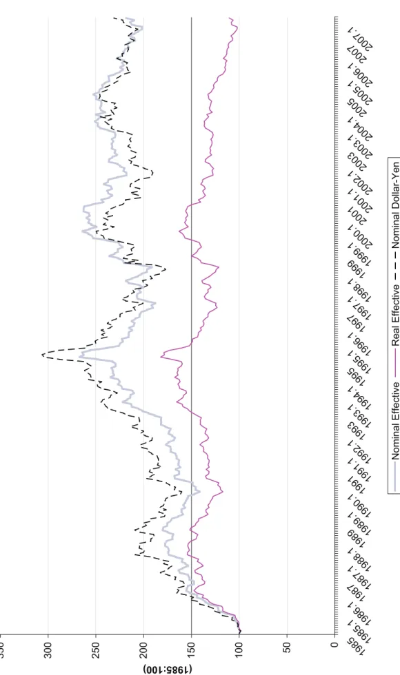
these policies, by February 1986, the yen-dollar exchange rate approached 180, from
about 250 before the Plaza Accord (Figure 1). The yen continued to appreciate, reaching
120 in early 1988. There was another spurt of appreciation in early 1995, with the yen
momentarily touching below 90. Subsequently, the yen weakened to as much as 130,
although it has mostly been in the 110-120 range during the last decade, except for the
period after the fall of 2008, when the yen briefly touched below 90 again.1 These trends
in the Japanese currency apply also in terms of the Nominal Effective Exchange Rate
(NEER), although in terms of the Real Effective Exchange Rate (REER), the yen
appreciation was more muted, with the REER back at pre-Plaza levels by early 2007.
In this paper, we focus on the movements of the yen on Japanese industries, and
on the sectoral reallocation of Japanese employment. We show that the appreciation
episodes of 1985 and 1995 have significantly hurt the ability of Japanese industries to
compete with U.S. industries, by raising the relative production costs of Japanese
industries. This relative cost gap with U.S. industries narrowed from 1995, owing to
faster wage growth in the U.S., and especially to higher productivity growth in some
Japanese industries. In fact, in these high productivity Japanese manufacturing industries
such as chemicals and transport equipment, relative production costs were essentially
back to pre-1985, pre-Plaza Accord levels by 2004. In contrast, the relative production
1
The effects of the Global Financial Crisis of 2008 on the yen-dollar exchange rate and on the competitiveness of Japanese industries are too recent to be analyzed in this paper.
costs of Japanese low productivity manufacturing industries such as textiles and wood
products have remained high. Clearly, in the aggregate, the appreciation of the yen was
not matched by an increase in Japanese productivity.
What then is the appreciation of the aggregate real exchange rate consistent with
these Japan-U.S. differences in industrial productivities? To answer this question, we
build a three-sector (high productivity manufacturing, low productivity manufacturing,
and services) equilibrium macroeconomic-trade model of Japan and the U.S. We find
that while the yen was “undervalued” before 1985, it was significantly “overvalued” after
1985, and especially since 1995. In our model simulations, the Balassa-Samuelson effect
is observed: the equilibrium real exchange rate is appreciating over time, owing to strong
relative growth in the Japanese high productivity manufacturing sector, but very poor
relative productivity growth in the Japanese services sector. Interestingly, the continued
appreciation of the equilibrium real exchange rate meant that the actual real exchange
rate was near its equilibrium value by early 2003, when the nominal yen dollar rate was
about 120 yen to the dollar.
Finally, we use our model to examine the relationship between these Japan-U.S.
differences in average production costs and the allocation of employment across the three
sectors. In both Japan and in the U.S., “de-industrialization” or the rise of the service economy is of important policy concern. While our model simulations follow the decline
in the employment shares in high productivity manufacturing quite well, our model fails
to capture the large flow of employment from low productivity manufacturing to services
in both countries. This failure is not simply because our long-run model cannot capture
mirror image of the yen—was ―”undervalued” against the yen, but the U.S. also
experienced a decline in employment in low productivity manufacturing. We suggest that
some third long-term structural factor, such as the rise of China and India may be
responsible for the surge in service sector employment in Japan and in the U.S.
As noted by Hamada and Okada (2007) and McKinnon and Ono (1997), the Plaza
Accord shifted the exchange rate expectations of market participants upwards, towards a
sharp yen appreciation. After the Accord, market participants became convinced that the
U.S. and Japanese governments would continue undertake policies to appreciate the yen,
as long as Japanese trade surpluses—especially against the U.S.-- remained large. The yen continued to appreciate, reaching a peak of slightly under 90 yen in 1995. Given the
sluggishness in the adjustment of prices, the real exchange rate appreciated in tandem.
This appreciation of the real exchange rate made Japanese industries
uncompetitive against comparable U.S. industries. The competitive discrepancy was
adjusted over time, through changes in relative Japan-U.S. wages, capital costs, or
differential rates of technical progress. In the long run, these adjustments, collectively,
should restore the real exchange rate to its equilibrium value. However, the restoration of
the real exchange rate to its equilibrium would typically take a very long time.2
As mentioned, in our model, the long- or very long-run equilibrium real
exchange rate is determined largely by the Balassa-Samuelson effect, that is, the
productivity differentials between Japan and the U.S. Japan’s real exchange rate
2Empirically, the speed at which the real exchange rate reaches equilibrium parity is very
slow. According to Froot and Rogoff (1995), standard estimates of the real exchange half-life lie in the range of three to five years. In our macroeconomic-trade model, we show that it was only in 2003 when the real exchange rate was restored to its equilibrium value—almost a full 20 years after the Plaza Accord.
appreciates over time, because of the very rapid productivity growth in Japan’s high productivity manufacturing sector relative to the country’s unproductive services sector.
In contrast, in the U.S., the gap in productivity growth between the high productivity
manufacturing and the services sectors is not as large.
Compared to our long- to very long-run analysis of Japan-U.S. real exchange
rates, Lane (2008, this volume) is concerned with more medium-run movements in
Japan’s real exchange rate. In the medium-run, large creditors such as Japan will
experience an appreciation of its real exchange rate, as net investment inflows lead to an
excess of domestic absorption relative to domestic production (“the transfer effect”). In our very long-run model, trade is balanced and there is no “transfer effect.”
Obstfeld (2009, this volume) characterizes Japanese real exchange rates from the
short- to the long-runs, and depicts how business cycles and monetary policies can
change real interest rates, and cause the short-run real exchange rate to deviate from its
long-run value. Obstfeld shows that the Balassa-Samuelson effect would appear to hold
in the long- to the very long-runs, although empirically it may take more than 20 years—
which is the length of time it takes in our model—for the real exchange rate to revert to its equilibrium value. Neither Lane nor Obstfeld examine the effects of exchange rates on
Japanese industries, or on Japanese sectoral employment, as we do in this paper.
In the next Section, we first analyze how the high yen raised the production costs
of Japanese industries relative to those in U.S. industries.3 We will compare—in dollar terms--the average production costs of 14 Japanese and U.S. manufacturing industries.
We show that Japanese average costs at the industry level have risen substantially
3
See also Dekle (2005) for an analysis using firm level data on how the high yen has hurt the profitability of Japanese firms.
between 1985 and 1995.4 Since then, Japan-U.S. gaps in average costs have narrowed
somewhat, largely owing to more rapid wage increases in the U.S. In some key Japanese
industries, productivity growth was rapid, helping close the average cost gaps with U.S.
industries. These Japanese high productivity industries were in optics, transport
equipment, and chemical products. In these and in some other industries, Japanese
average costs in terms of dollars were almost the same as U.S. average costs by 2004. In
industries in which Japanese productivity growth were relatively low, such as rubber and
plastics, and textiles and apparel, the gaps in average costs between Japanese and U.S.
industries remained substantial even in 2004.
In Section III, we build a simple long-run Ricardian Japan-U.S.
macroeconomic-trade model that endogenizes the real exchange rate and wage responses.5 The model has
three sectors: the low and high productivity manufacturing sectors, and the services
sector. We use the Japan-U.S. productivity levels calculated from the EU KLEMS data,
and feed the productivity levels data into our model. Using our model and the
productivity data, we simulate the Japan-U.S. real exchange rates, average costs, and
sectoral employment shares. Our simulated Japan-U.S. real exchange rates can be
interpreted as an equilibrium benchmark that depends mostly on relative productivity
differences between Japan and the U.S. (and model parameters). This benchmark can be
4 In related work, Jorgenson and Nomura (2005) calculate using detailed commodity level prices, the
purchasing-power parity (PPP) exchange rates between Japan and the U.S., and found that for many of the 42 industries examined, the actual yen-dollar exchange rate was much higher than the PPP exchange rates.
5 The analysis at the industry level is of the short to medium-runs, at a horizon when real exchange rates
can still be deviating from fundamentals, say, owing to a monetary or expectations shock. In the long-run, exchange rates and relative Japan-U.S. wages are both endogenous. For example, a positive productivity shock to the Japanese manufacturing sector will appreciate the Japanese real exchange rate and raise economy-wide Japanese wages. The appreciation of the yen and the increase in Japanese wages will raise average costs in Japanese manufacturing. The net effect of the positive productivity shock on Japanese manufacturing average costs is thus ambiguous in the long-run.
used to assess whether actual Japan-U.S. real exchange rates are “misaligned.”6 We focus on understanding the changing sectoral employment shares in Japan and in the
U.S., given the widespread policy interest in the “de-industrialization” of the manufacturing sector and the rise of services sector in both countries.
We find that our baseline model simulations follow the Japan-U.S. real exchange
rates, and the Japan-U.S. gaps in average costs in both the low and high productivity
manufacturing sectors quite well over the long-run. As is expected in our static, long-run
framework without money, we miss most of the short-run fluctuations. With regards to
the sectoral employment shares, our baseline model simulations follow the employment
shares in high productivity manufacturing quite well, and in the services sectors
somewhat well, but fail to follow the employment shares in the low productivity
manufacturing sector.
II. The Changing Relative Average Production Costs of Japanese Industries versus U.S. Industries since 1985.
In this Section, we will analyze how the “competitiveness” or U.S.-Japan relative average costs) have changed over time. We measure changes in the competitiveness of
Japanese industries by estimating the changes in their average costs of production in
comparison with the changes in the average cost of production of U.S. industries. The
change in average costs can be decomposed into the change in capital costs, the change in
wages, the change in the cost of input materials, and finally, the change in total factor
productivity.
6
In Obstfeld and Rogoff (2005) and Dekle, Eaton, and Kortum (2008) the equilibrium real exchange rate is defined as the rate at which the current accounts in all countries would be equal to zero.
II.1: Methodology and the Data.
We begin by explaining our methodology and basic assumptions. Suppose that
there exists a well behaved constant returns to scale production function for a
representative firm in industry i of country J of the following form:
)) ( ), ( ), ( ), ( ( ) ( , , , , , , t F L t K t X t T t YiJ = iJ iJ iJ iJ iJ (1)
where YiJ(t) denotes the real gross output of this firm at time t, LiJ(t) is the labor input,
KiJ(t) the capital service input, XiJ(t) the input of intermediate goods, and T iJ(t) the
technology level.
The average cost of production of this firm, CiJz(t), is expressed by
) ( ) ( ) ( ) ( ) ( ) ( ) ( ) ( , , , , , , , , t Y t X t q t K t r t L t w t C J i J i J i J i J i J i J i J i + + = (2)
where wiJ(t) denotes the nominal wage rate (measured in country J’s currency) for
workers in industry i of country J at time t, riJ(t) represents the capital service price, and
qi,J(t) the intermediate input price. We assume that each firm is a price taker in all factor
markets. We also assume that factor prices and the technology level, TiJ(t), are continuous
functions of time.
By differentiating equation (2) over time and using cost minimization conditions, we
obtain ) ( ˆ ) ( ˆ ) ( ) ( ˆ ) ( ) ( ˆ ) ( ) ( ˆ , , , , , , , , , , , t s t w t s t r t s t q t A t CiJ = LiJ iJ + KiJ iJ + XiJ iJ - iJ (3)
where the circumflex accents denote the growth rate of variables. sL, i,J(t), sK, i,J(t), and
) ( ) ( ) ( ) ( ) ( ) ( ) ( ) ( ) ( ) ( ) ( ) ( ) ( ) ( ) ( ) ( ) ( ) ( ) ( ) ( ) ( ) ( ) ( ) ( ) ( ) ( ) ( , , , , , , , , , , , , , , , , , , , , , , , , , , , , , , t X t q t K t r t L t w t X t q t s t X t q t K t r t L t w t K t r t s t X t q t K t r t L t w t L t w t s J i J i J i J i J i J i J i J i J i L J i J i J i J i J i J i J i J i J i L J i J i J i J i J i J i J i J i J i L + + = + + = + + =
Ai,J(t) denotes the total factor productivity (TFP) level of industry i in country J at
time t. The TFP growth rate can be defined by
) ( ) ( ) ( ˆ , , , , , t Y dt t dT T F t A J i J i J i J i J i ¶ ¶ =
Using growth accounting, we can estimate the TFP growth rate.
Equation (2) shows that we can explain the relative competitiveness (which we
measure by the gap in the average costs of production) of the two countries in each
industry by the gap in factor prices between the two countries and the gap between their
TFP levels.
In order to apply equation (2) to discrete time-series data, we use a Tornqvist-type
approximation of this equation:
))) 1 ( ln( )) ( (ln( ))) 1 ( ln( )) ( (ln( 2 ) 1 ( ) ( ))) 1 ( ln( )) ( (ln( 2 ) 1 ( ) ( ))) 1 ( ln( )) ( (ln( 2 ) 1 ( ) ( )) 1 ( ln( )) ( ln( , , , , , , , , , , , , , , , , , , , , , , -+ + -+ + -+ = -t A t A t q t q t s t s t r t r t s t s t w t w t s t s t C t C J i J i J i J i J i X J i X J i J i J i K J i K J i J i J i L J i L J i J i (4)
We can measure the inter-temporal changes in the competitiveness of industry i in
country J in comparison with that of industry i in country U by the changes in the ratio of
the average cost of production in the two countries measured in the same currency:
e(t)(C i,J(t) / C i,U* (t)), where e(t) denotes the nominal exchange rate index between the
currencies of the two countries (the value of country J’s currency in terms of country U’s
currency). We use year 1980 as the benchmark year and set e(1980)=100.
Here, we briefly explain our data. Details on data construction are given in
Appendix 1. We have data on 19 industries in both countries, 13 in manufacturing, 6 in
services. Data on the following factor inputs and on the TFP growth rate were obtained
from the EU KLEMS Database (March 2008 version).
wiJ(t)LiJ(t): nominal labor compensation in industry i in country J;
wiJ(t): labor compensation divided by the quality adjusted labor input index
(1995=100) of industry i in country J;
qiJ(t)XiJ(t): nominal intermediate input cost of industry i in country J;
qiJ(t): intermediate input cost divided by the real intermediate input index
(1995=100) of industry i in country J; and
ln(AiJ (t)−ln(AiJ(t−1)): TFP growth rate of industry i in country J.
We estimated the service price of capital as follows:
ri,J(t)=gross fixed capital formation price index (all assets, 1995=100) × (interest
rate + depreciation rate – capital gains)
We obtained the gross fixed capital formation price indices from the EU KLEMS
Database. We calculated the capital gain terms from these indices. For interest rates, we
on 10-year US Treasury securities for the US. Depreciation rates were obtained from the
Japan Industrial Productivity (JIP) Database for Japan and from the BEA website for the
U.S. To measure capital service inputs, we used the real capital stock in 1995 prices from
the EU KLEMS Database. For the yen-dollar exchange rates, we used the annual average
interbank market exchange rate from Nikkei NEEDS.
II.2: Japan-U.S. Productivity and Average Cost Comparisons.
If the appreciation of Japan’s real exchange rate (Figure 1) had been accompanied by superior productivity growth in comparison with other countries, then the appreciation
of the Yen until the mid-1990s would not have reduced the international competitiveness
of Japan’s manufacturing sector. However, in many manufacturing industries, the TFP growth achieved was not sufficient to cancel out the effects of the Yen appreciation. In
particular, from the 1990s, Japan’s TFP stagnated and Japan’s manufacturing industries lost in competitiveness.
Figure 2 compares the TFP growth of manufacturing industries in Japan and in the
U.S. In the period 1980-1990, TFP growth rates in most manufacturing industries in
Japan were higher than those in the U.S. However, during 1990-2004, TFP growth in
almost all manufacturing industries became very low in Japan, with the exception of the
electrical and optical equipment industries, and U.S. TFP growth in most manufacturing
industries exceeded Japan’s.
Figure 3, Panel A shows how average production costs have changed over time in
Japan and in the U.S. in the electrical and optical equipment industry. Production costs
will fall when there is a decline in wages, capital costs, materials costs, or a rise in TFP.
shows that holding the yen constant, Japanese production costs in the electrical and
optical equipment industry have trended along with U.S. production costs. However, in
terms of dollars, Japanese production costs in this industry surged after the yen
appreciation in 1985, reaching a peak at about 1995. Thereafter, Japanese production
costs in terms of dollars started to decline, gradually approaching U.S. levels by 2005.
To see the role of wage rate and productivity changes on Japan-U.S. relative average
production costs, Figure 3, Panel B shows that relative to Japanese wages, U.S. wages
have surged, especially since 1995, contributing to the convergence of Japan-U.S.
average costs. Japanese TFP growth rates have generally been lower than U.S. TFP
growth rates, except for the period after 2002 in the electrical and optical equipment
industry.
Figures 4, 5, 6, and 7 depict similar data for the rubber and plastics, the textiles,
apparel, leather and footwear, the transport equipment, and chemicals and chemical
products industries, respectively.7 Generally, the patterns observed in these industries are
similar to the pattern observed in the electrical and optical equipment industry. First, the
yen appreciation sharply deteriorated the competitiveness of Japanese industries, starting
in 1985. However, the rapid increase in U.S. wage rates has partially offset the drop in
Japanese competitiveness. The decline in capital cost and intermediate input prices in
Japan (unreported, to conserve space), also contributed to offsetting the effect of the yen
appreciation.
7We created similar figures for other manufacturing industries (general machinery; basic and fabricated
metals; other non-metallic minerals; coke, refined petroleum and nuclear fuel; food, beverages and tobacco; wood and of wood products; pulp, paper, printing and publishing; and manufacturing not elsewhere classified and recycling). However, to conserve space, we omit these figures.
Second, Japan’s competitiveness relative to the U.S. reached bottom in 1995. This result is consistent with the fact that Japan’s real effective exchange rate (REER) was most appreciated in 1995 (along with the yen-dollar rate and the nominal effective
exchange rate) (Figure 1). After that, the yen gradually depreciated in REER terms, and
by 2006 the real effective exchange rate approached the level of the level of 1985.
Third, in industries where Japan’s TFP growth were on par with or higher than that of the U.S. (before 1990) such as electrical and optical equipment, transport equipment,
chemicals and chemical products, general machinery, and pulp, paper, printing and
publishing, the Japan-U.S. average cost gap in dollars did not become very large even in
1995, and becomes negligible by 2004. On the other hand, in industries where Japan’s TFP growth was much smaller than that of the U.S. before 1990, such as rubber and
plastics, textiles, apparel, leather and footwear, basic metals and fabricated metal, and
food, beverages and tobacco, the Japan-US gap in the average cost of production
measured in dollars became very large in 1995, and even now remains sizable.
III. Japan-U.S. Productivity Differences, Real Exchange Rates, and Sectoral Employment Shares in the Long-run: A Three-Sector, Two-Country Model.
The previous Section showed that as the yen appreciated, Japanese average
production costs rose relative to U.S. average production costs, on an
industry-by-industry basis. The relative rise in Japanese average costs was larger in industries where
the increases in TFP growth were lower. For example, after the yen appreciation,
Japanese average costs rose substantially relative to U.S. average costs in textiles--a low
Japanese average costs relative to U.S. average costs were relatively constant over time.
The analysis in the previous Section is of the short- to medium-runs, when
nominal exchange rates can deviate from their Purchasing Power (PPP) values. In the
short- to medium-runs, tight monetary policies in Japan can appreciate the yen and raise
Japan’s relative average costs, as it happened in Japan between 1990 and 1995 (Hamada and Okada, 2008). However, in the long-run there is a tendency for Purchasing Power
Parity to hold in the sense that nominal exchange rate changes approach the changes in
relative prices (Taylor and Taylor, 2004). Thus, there is likely to be movement of
nominal exchange rates towards purchasing power parity within our sample period of 20
years or more. The real exchange rate simulated by our long- to very long-run model
below should be viewed as an equilibrium benchmark by which the “overvaluation” or the “undervaluation” of the actual real yen-dollar exchange rate can be evaluated.
We will focus on the impact of productivity differences between Japan and the
U.S. on Japan-U.S. real exchange rates and Japanese sectoral employment patterns. To
adequately analyze the impact of productivity differences on real exchange rates and the
allocation of employment across sectors, we need a general equilibrium model. A
negative shock to Japanese productivity will on the one hand, directly raise average costs
by lowering efficiency, while on the other hand, lower average costs by lowering wages
and depreciating the Japanese yen. Thus, a productivity shock has offsetting effects on
average costs, and it is unclear which effect will dominate in a partial equilibrium setup.
Moreover, industry-by-industry average cost comparisons cannot give a complete picture
a third sector--such as the services sector—can alter the Japanese manufacturing sector’s “competitiveness” through the Balassa-Samuelson effect.
We aggregate our 19 industries from the EU-KLEMS data described in Section II
and in Appendix 1 into 3 sectors, the 1) low labor productivity manufacturing sector, the
2) high labor productivity manufacturing sector, and the 3) services sector. In our model,
there are two countries, Japan and the U.S. and they each produce and consume the goods
in the 3 sectors. The manufacturing sectors in the two countries are differentiated. In fact,
we find after calibrating from the data, that Japanese low (and high) productivity
manufacturing and U.S. low (or high) productivity manufacturing goods have very low
substitutability in the consumption decisions of Japanese and U.S. households.8
III.1: Aggregating the 19 Industries into 3 Sectors and the Data on Sectoral Labor Productivities.
The model is a simple Ricardian type with no capital and labor as the only factor
of production, Yij=Ɵij Lij, where Ɵ݆݅ is labor productivity in industry i and country j.9 We
can relate Ɵ݆݅ to TFP ij in the previous Section if the production function is
Cobb-Douglas, since then Ɵ in each industry (omitting the subscripts) is equal to ܣͳെߙͳ ቀݎ
ߙቁ
ߙ
ͳെߙ
,
where 1-α is the labor share of income, r is the real rate of interest, assumed constant, and A is the level of TFP. The growth in labor productivity is then simply equal to:
8 The calibrated (Armington) elasticities between Japanese and U.S. low productivity goods and high
productivity goods are 0.897 and 0.877 respectively (Table A1 in Appendix 2). These calibrated elasticities
are lower than the values of 3 to 6 used in Obstfeld and Rogoff’s (2007) simulations.Our model also
allows for “home production,” which captures socio-economic phenomena such as the decline in
housework and child- and elder-care by Japanese households. These phenomena will increase the demand for non-tradeable services, and raise the relative price of services in Japan, thereby helping appreciate the equilibrium real exchange rate (Messina, 2006).
9
gr(Ɵ)= ͳ
ͳെߙ݃ݎሺܣሻǤ Using the growth in TFP by industry and the labor shares by industry
calculated in the previous Section (from EU-KLEMS) and described in Appendix 1, we
can then calculate the growth in labor productivity for each of our 19 sectors (13 in
tradeables manufacturing, 6 in nontradeable services).
We rank each of our 13 industries in manufacturing according to the average
growth of Japanese labor productivities in these industries between 1978 and 2003. As a
result of this ranking procedure, we classify the following six manufacturing industries as
“Low Productivity Industries” (these industries had the six lowest average labor productivity growth rates): 1) food, 2) textiles, 3) wood, 4) pulp and paper, 5) refined
petroleum, and 6) basic and fabricated metals. We classify the following seven
manufacturing industries as “High Productivity Industries”: 1) chemicals, 2) rubber, 3) non-metallic metals, 4) basic machinery, 5) electronics and optical machinery, 6)
transport equipment, and 7) manufacturing not elsewhere classified. The “Services
Industries” include 1) hotels, 2) transport and storage, 3) posts and telecommunications, 4) financial intermediation, 5) real estate, and 6) other business services.
To simulate our model, we need data on labor productivity, labor supply, output
(in dollars), and prices (in dollars) for each of our three sectors, for both Japan and the
U.S. Labor supply is defined as the total number of hours worked in that particular
sector. Labor productivity is thus in terms of “output per hour.” For each of the three sectors, we form weighted averages of the data for the industries that comprise that
particular sector, where the industry’s output share in that sector is used as the weight for that industry.
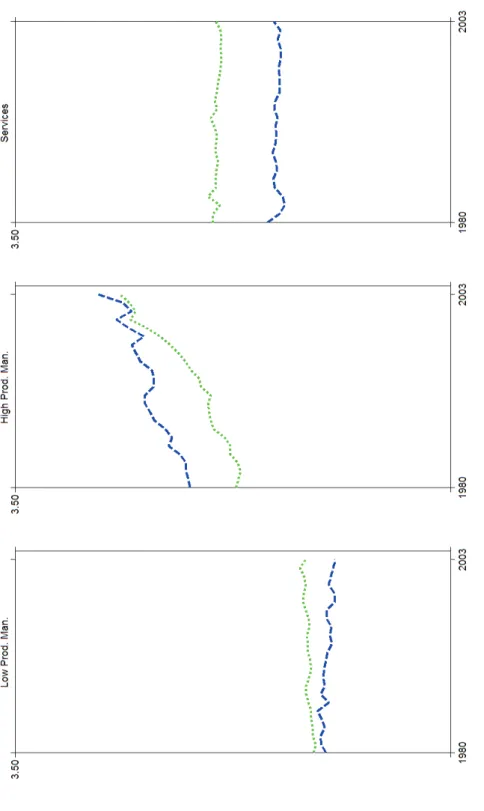
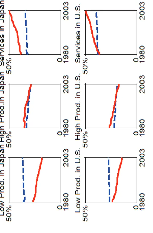
Figure 8 depicts the data for labor productivities so constructed from 1980 to
2003. This is the data that we feed into the model to simulate our series for the
Japan-U.S. relative average costs, the Japan-Japan-U.S. real exchange rate, and the sectoral labor
shares. The units are in terms of the numeraire sector, Japanese Low Productivity
manufacturing. (Labor productivity in 1980 in the Japanese Low Productivity sector is set
to unity.) Thus, we can compare labor productivity levels not only between Japan and the
U.S., but also across the three sectors. We can see from the Figure that in the “Low Productivity Industries,” labor productivity in Japan was declining slightly during this
period, while in the U.S., labor productivity was rising. In the “High Productivity Industries,” labor productivity growth was high in both countries, especially in the U.S.
until about 1997. Since then, Japanese labor productivity growth has outstripped U.S.
labor productivity growth in this sector, especially since 2000. In Services, labor
productivity growth in both countries was flat. The level of labor productivity in Services
in Japan compared to that in the U.S. is especially low.
III.2: The Balassa-Samuelson Effect and Real Exchange Rates.
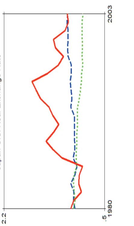
In Figure 9, we compare the real exchange rate in the data, with the real exchange
rate simulated from the model. For the data, the real exchange rate is defined as the ratio
of the weighted GDP deflators in the two countries in terms of dollars. To convert the
Japanese GDP deflator into dollars, we use 1) the nominal yen-dollar exchange rate, and
2) the yen-dollar exchange rate adjusted for Purchasing Power Parity (from Heston,
Summers, and Bettina, 2006). The model simulated real exchange rate, the market real
equal around 1980. That is, all three exchange rates are assumed to be in equilibrium in
1980.
In the model, the real exchange rate is defined as the ratio of the weighted
averages of the three sectors in Japan and in the U.S., in terms of a common numeraire, in
our case, the Low Productivity manufacturing sector in Japan. Since in the data, the gap
in productivity growth between services and in manufacturing is wider in Japan than in
the U.S. (from Figure 8), we should find aggregate prices in Japan rising faster than
aggregate prices in the U.S. (the Balassa-Samuelson effect).
Figure 9 shows that in the long- to very long runs, the real exchange rate as
simulated from our model matches the data well, especially when the nominal yen-dollar
exchange rate is used to convert the Japanese GDP deflator to U.S. dollars. Specifically,
we observe the Balassa-Samuleson effect-- an appreciation of the Japanese real exchange
rate over the long-run. (Unsurprisingly, in our model with no money and no price
rigidities, we miss most of the short- and medium-run fluctuations in the real exchange
rate.) If we take our simulated real exchange rate series as a long-run benchmark, we
find that the actual real exchange rate was “undervalued” until 1985, but was
“overvalued” between 1986 and 2000. Note that by 2003, while the yen is “overvalued”
in comparison to the Heston, Summers, and Bettina PPP real exchange rates, it is slightly
“undervalued” in comparison to our model simulated real exchange rates. Obstfeld (2009, this volume) shows that over the short- to medium-runs,
deviations from the Balassa-Samuelson benchmark are substantial. Lane (2008, this
volume) finds that the yen-dollar exchange rate is cointegrated with Japan-U.S.
long-runs. We find more evidence than does Obstfeld that the yen-dollar real exchange
rate reverts to its benchmark equilibrium over the long-run. This is probably because our
model used to simulate the equilibrium benchmark is somewhat more general than the
usual Balassa-Samuelson model, where the real exchange rate depends only on the two
countries’ “difference in differences” between their tradeable-sector and nontradeable-sector productivity growth rates. In our model, in addition to the usual
Balassa-Samuelson productivity differentials, we have three rather than two sectors, with each
sector—for example, the Low Productivity manufacturing sector—producing highly differentiated goods in Japan and in the U.S. We also have “home production” in each
country, which, given our parameter values (in Table A1), will tend to raise the relative
price of Services in Japan, resulting in an appreciation of the model simulated real
exchange rate that better matches the long-run appreciation of the actual yen-dollar real
exchange rate.
III.3: Sectoral Average Costs and Sectoral Employment Shares.
Average cost in our framework is equal to: κͳ
ܣቀ ݓ
ͳെߙቁ
ͳെߙ
, where in both countries,
κ is a constant, and w are wages in dollars. As in the previous Section, average costs in Japan will rise relative to average costs in the U.S. when 1) Japanese productivity growth
is lower than U.S. productivity growth; or 2) when Japanese wages grow faster than U.S.
wages, either because of faster wage growth, or because of an appreciation of the yen,
which raises Japanese wages in dollar terms. Note, however, that both w and the real
dollar-yen exchange rates depend on economy-wide labor productivities, including
Services sector lowering Japanese relative wages, but appreciating the yen. Thus, the net
effect of productivity growth on Japan-U.S. average costs is ambiguous.
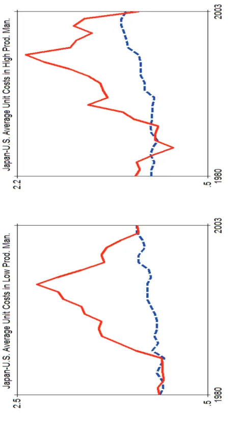
In Figure 10, we depict the ratios of Japanese average costs to U.S. average costs,
both in the data and in the model. As in the previous Section, in the data, Japanese
average costs rise sharply relative to U.S. average costs starting from about 1985 and
peaking around 1995. From 1995, the closing of Japan’s average cost gap with the U.S. is
much slower in the Low Productivity sector, because Japan’s productivity growth is lower than in the U.S. in this sector. Thus, the closing of the average cost gap occurs
entirely due to the rise in relative U.S. wages. By 2003, in the High Productivity
Industries, average costs in Japan relative to those in the U.S. are lower than even in
1980, signifying the sharply improved competitiveness of Japanese High Productivity
Industries since 1995. This is not only because of higher Japanese productivity in this
sector, but also because of the rise in relative U.S. wages. (Recall that since there is full
inter-sectoral mobility of labor, wages in all three sectors are equalized. Economy-wide
wages are determined by trade patterns and within country aggregate productivity,
including productivity in Services, which is higher in the U.S.)
The model tracks the long-run trends in the relative costs quite well, although we
miss the yen appreciation episodes between 1985 and 1995. As mentioned, these are
clearly episodes when the nominal yen appreciation departed from the economic
fundamentals of Japan, and our model, driven entirely by productivity growth and other
fundamentals, cannot capture these episodes.
We have shown that slower relative productivity growth in the Services Industries
the faster growth of productivity in tradable goods, the decline in employment in the
manufacturing sectors of industrialized countries—the so-called “de-industrialization
hypothesis.” The economic reasoning is simple: with fewer workers able to produce a higher volume of manufacturers, some workers will have to switch jobs to Services.
As Obstfeld and Rogoff (1996, Ch. 4) and Matsuyama (2008) point out, however,
this simple reasoning does not account for the fact that demand for and thereby
employment in manufacturers in a particular country may fall off, owing to the decline in
their price in the global market, because of oversupply or increased global competition.
The change in manufacturing employment generally depends in a complicated way on
sectoral demand elasticities, both domestic and abroad. That is, the “de-industrialization
hypothesis” focuses on technological change and within country productivity growth, but generally ignores the impact of international trade.
The “de-industrialization hypothesis” should be examined in at least a two-country general equilibrium framework with endogenously evolving relative prices.
Below we depict simulations of the changes in the labor shares in both Japan and in the
U.S., using our model’s calibrated elasticities. We also compare our model simulations with what actually happened to the labor shares in the three sectors in Japan and in the
U.S. between 1978 and 2003.
For our parameter values (in Table A1), the model predicts that employment
shares of the High Productivity Industries in both countries should be decreasing. The
employment shares in the Low Productivity Industries and in the Services Industries
should be increasing (Figure 11). Our model tracks the actual employment shares in High
employment shares in the Services Industries are increasing more sharply in the data than
in the model. Also, in the data, the employment shares in Low Productivity
manufacturing are declining dramatically, while in the model, these shares are increasing.
Thus, while our model captures the trends in the High Productivity Industries
reasonably well, our model fails to capture the downward trend in employment in the
Low Productivity Industries, and upward trend in employment in the Services Industries.
In particular, our model fails to capture in both countries, the dramatic actual movements
of labor from Low Productivity manufacturing to the Services sector. Our model’s
simulation results are robust to raising the Armington elasticities in the Low Productivity
Industry to 1.5; and to raising the consumption utility weightsg1i of Low Productivity
goods from 0.1 to 0.2 or 0.3 in both countries.
Why does our model fail in this important dimension? In both the U.S. and in
Japan, actual productivity growth in Low Productivity manufacturing is just too low to
drive out labor to the Services sector. In our model, we would need labor productivity
growth in Low Productivity manufacturing of over 4 percent per year to have sufficient
labor migration from the Low Productivity sector to the Services sector, a rate of labor
productivity growth much higher than what is observed in the data of both countries.
The failure of our model is not simply because our long-run model cannot capture
the temporary employment effects of the “overvaluation” or “misalignment” of the yen. The dollar—the mirror image of the yen—was “undervalued” against the yen, but the U.S. also experienced a decline in employment in Low Productivity manufacturing. The
the decline in low productivity manufacturing employment in both countries. There must
be some other factor.
The other factor may be the rise of India and China, countries that are specialized
in industries such as textiles and apparel, industries which are classified as “Low Productivity” manufacturing in Japan and in the U.S. As Broda and Weinstein (2008) note, in 1992, the U.S. exported three times as much to Japan as China; by 2005, China
was exporting twice as much to Japan as the U.S. Thus, China today may be a more
important trading partner to Japan than is the U.S. As Coleman (2007) points out, the
rise of these Giants can theoretically lead to de-industrialization in industrial countries
such as Japan and the U.S. An interesting empirical exercise using our basic framework
would be to combine China, India, and the U.S. into the “rest-of-the-world,” and examine how the changing sectoral labor productivities in the “rest-of-the-word” would impact the evolution of Low Productivity manufacturing in Japan.
IV. Conclusion.
The main objective of this paper is to try to better understand the relationships
among Japanese productivity growth, the Japan-U.S. real exchange rate, and long-run
economic outcomes, such as Japanese employment. As the yen appreciated starting in
1985, Japanese “competitiveness”--defined as the ratio of U.S. average costs to Japanese average costs—sharply declined. However, the decline in Japanese competitiveness differed among industries. In industries where Japanese productivity growth was
A comparison of the actual real exchange rate with this paper’s long-run
equilibrium benchmark shows that the Japanese real exchange rate was near equilibrium
in 2003, when the nominal yen-dollar exchange rate was around 120 yen to the dollar.
The recent rapid appreciation of the yen to below 90 yen to the dollar, owing to the
Global Financial Crisis is thus clearly excessive, and has resulted in large profit and
employment losses for Japanese manufacturers. Our analysis suggests that a return of the
Appendix 1: Definition of Variables Used in the Empirical Analysis and Data Sources
The purpose of this Appendix is to provide an explanation of the data which we used for our empirical analysis.
Quantities and Prices of Output and Factor Input by Sector
In the case of output and intermediate input prices and quantities by sector, we used the EU KLEMS Growth and Productivity Accounts (March 2008 Release, downloadable at http://www.euklems.net/). A detailed explanation of the methodology and data sources of the EU KLEMS can be founded in Timmer et al. (2007a and 2007b). The major data source for the EU KLEMS Accounts on Japan is the Japan Industrial Productivity (JIP) Database (downloadable at http://www.rieti.go.jp/en/database/ JIP2008/index.html). A detailed explanation of the methodology and data sources of the JIP Database can be founded in Fukao et al. (2007). The most recent version of the JIP Database, JIP 2008, was jointly compiled by the Research Institute of Economy, Trade and Industries (RIETI) and Hitotsubashi University. Original data for the EU KLEMS Accounts on the United States are provided by the Bureau of Economic Analysis and Dale Jorgenson of Harvard University and scholars who joined his project.
The EU KLEMS Accounts provide nominal and real values and implicit price indices of gross output, value added, and intermediate inputs for about seventy sectors, which cover the whole economy of Japan and the United States. For the aggregation of these indices, the Tornqvist method was used. The original sources for these data are the SNA statistics for Japan and the United States as well as background data such as input-output tables.
Assuming constant returns to scale, fully competitive factor and output markets, and full utilization of
factor inputs, the TFP growth rate in sector i of country J is derived using standard growth accounting:
) ( ˆ ) ( ˆ ) ( ) ( ˆ ) ( ) ( ˆ ) ( ) ( ˆ , , , , , , , , , , , t t L t t K t t X t A t QiJ =nLiJ iJ +nKiJ iJ +nXiJ iJ + iJ (A1)
where the circumflex accents denote the growth rate of variables (the inter-temporal change of each log
value from t to t+1). Qi,J(t), Li,J(t), Ki,J(t), Xi,J(t), and Ai,J(t) denote gross output, labor service input, capital
service input, intermediate input, and the TFP level respectively. νL, i,J(t), νK, i,J(t), and νX, i,J(t) denote the
compensation share of each production factor.
The growth rate of capital service input is derived by weighting the growth of each type of fixed asset
by the share of each asset’s capital cost in total capital cost as follows:
å
= k iJ k J i k J i t t S t Kˆ, ( ) n ,, ( )ˆ ,, () (A2)where νk, i,J(t) denotes the share of capital cost of asset k in total capital cost and S k, i,J(t) denotes the stock of
asset k, which is estimated by applying the perpetual inventory method and geometric depreciation rates on
investment flow data by industry and by asset. Three types of ICT assets (office and computing equipment, communication equipment, and software) and four types of non-ICT assets (transport equipment, other machinery and equipment, residential buildings, and nonresidential structures) are treated as different types of assets.
The growth rate of labor service input is derived by weighting the growth of man-hour input of each type of labor by the share of compensation for each type of labor in total labor compensation as follows:
å
= l J i l J i l J i t t H t Lˆ, () n ,, ( ) ˆ ,, ( ) (A3)where νl, i,J(t) denotes the share of compensation for type l labor in total labor compensation and Hl, i,J(t)
denotes the total hours worked by type l labor. For this calculation, data on hours worked and labor
compensation arecross-classified by the sex, education, an employment status of workers.
In our calculation of the cost share of each production factor for equation (3), we used the total labor compensation and total intermediate input cost in each industry, which are included in the EU KLEMS Accounts. In the case of capital cost, we did not use the capital compensation from the EU KLEMS Accounts. The reason is that capital compensation in the EU KLEMS accounts includes windfall profits and mark-ups. Instead, we estimated capital costs ourselves. Our method is explained below.
Capital Cost and Exchange Rates
The cost of capital by sector for the United States and Japan are calculated as follows:
Capital cost 㸻 user cost × real fixed capital stock (all assets, 1995 prices)
where the real fixed capital stock is taken from the EU KLEMS Accounts. The user cost of capital for each sector is derived by
User cost =gross fixed capital formation price index (all assets, 1995=100)
× (interest rate + depreciation rate – capital gain from fixed capital stock)
We obtained gross fixed capital formation price indices from the EU KLEMS Accounts. As interest rates for Japan, we used data on yields on newly-issued government bonds (10 years) downloaded from the Bank of Japan website (http://www.boj.or.jp/theme/ research/stat/market/bondmk/bondyield/index.htm). For the United States, we used the market yield on U.S. Treasury securities (10-year constant maturity, quoted on an investment basis) downloaded from the Federal Reserve Board website
(http://www.federalreserve.gov/datadownload/Choose.aspx?rel=H.15). We obtained the average depreciation rates of all assets for each industry from the JIP 2008 and BEA Data.
As yen-dollar exchange rates, we used the annual average value of the yen-dollar exchange rate data of Nikkei Economic Electronic Database Systems (NEEDS).
Appendix 2: The Two-County, Three-Sector Ricardian Model10
We develop a three-sector, two-country general equilibrium Ricardian model, two sectors produce traded goods and one sector produce non-traded good, in which goods are differentiated by the productivity with which they are domestically produced. This feature of the model, and the degree of substitutability in
preferences between home and foreign produced units of each good, endogenously determine a country’s
equilibrium pattern of production and trade. We denote two countries by “JP” and “US”. There is no
international labor mobility but perfect labor mobility across sectors.
Firms
There is continuum of firms producing each good. Firms behave competitively, taking the prices of the production goods and of the factor of production as given. Each good is produced using one factor of
production, labor, in linear technology, which is given by Yji =qijNij, for industry j in country i. Here
i j
q denotes the sector specific productivity that changes over time and Nij is the sectoral employment.
Productivities in the model are exogenous and are taken from the data. The problem confronted by sector j
in country i is the problem of maximizing profits subject to the production technology. The first order
conditions for the producers’ problem imply that the quantity of each good j produced and the quantity of
factors hired in the industry satisfy that wi = pijqij, where pij is the producer price of the good j in
country i and wi is the wage rate in country i.
Agents and Preferences
There is a representative agent in each country who consumes all three types of goods and works. Consumption is the only determinant of the utility function, which is given by
( )
( )( )
( )(
)
( 1) ( 1) 3 3 1 2 2 1 1 1 log -÷ ø ö ç è æ + + + = gi i s s gi i s s gi i i s s s s i s C C C U .Here C1i and C2i are determined by the Armington Aggregators and C3i is the non-traded good.
Specifically, C1i and C2i are given by
(
)
(
)
(
)
(
)
(
1)
(
1)
, 1 , 1 -úû ù êë é + -= j j i j j j j US j j i JP j j i j C C C e e e e e e m m .Parameter s is the elasticity of substitution between the different goods. Parameter si is the home
consumption of service activities (Messina 2006). The weights gij influence how consumption expenditure
is allocated across goods in each country. We use the Armington assumption: products from different
countries are imperfect substitutes. Parameter ej is the elasticity of substitution (Armington elasticity)
between domestically produced and imported goods for sector j. Parameter of bias in preferences towards
the goods produced in Japan is mj, whereas 1-mj represents the parameter of bias in preferences towards
the American goods. The representative consumer in Japan solves the problem of maximizing the utility subject to the following budget constraint
10
JAP JAP JAP JAP US US JAP US US JAP JAP JAP JAP JAP JAP w C p C p C p C p C p1 1, + 2 2, + 1 1, + 2 2, + 3 3 £ .
The representative consumer in the U.S. solves a symmetric problem.
Trade is balanced since there is no intertemporal lending/borrowing
JAP US US JAP US US US JAP JAP US JAP JAPC p C p C p C p1 1, + 2 2, = 1 1, + 2 2, .
Resource constraints for labor in each country are given byN1i +N2i +N3i =1. Resource constraints for
traded sectors are given by YjJP =CJPj,JP+CUSj,JP and YjUS =CUSj,US +CJPj,US . Resource constraint for
non-traded sectors are given by Y3JP =C3JPand Y3US =C3US.
The Real Exchange Rate
The bilateral real exchange rate at any date between Japan and the United States is given by RER=PUS PJAP
.The aggregate price index for country i is simply given by Pi =
(
YN1i +YN2i +YN3i) (
YR1i +YR2i +YR3i)
,where YNij is the nominal value added for sector j in country i, while YRij is the corresponding real value added in
that sector.
Table A1: Model Parameter Values
Sectoral Armington Elasticities (1, Low Productivity; 2, High Productivity)
ߝͳ=0.897 877 . 0 2 = e
Preference Bias Toward Japanese Goods (1, in Low Productivity; 2, in High Productivity) 439 . 0 1º m 425 . 0 2 º m Other Parameters ࢙ ൌെǤǡൌࡶǡࢁ U J i i , , 1 . 0 1 = = g U J i i , , 1 . 0 2 = = g U J i i , , 8 . 0 3 = = g
References
Broda, C. and D. Weinstein, 2008, “Exporting Deflation? Chinese Exports and Japanese Prices,” NBER Working Paper 13942.
Coleman, J., 2007, “Accommodating Emerging Giants,” mimeographed, Duke
University.
Dekle, R., 2005, “Exchange Rate Exposure and Foreign Market Competition: Evidence from Japanese Firms,” Journal of Business, 78 (1), pp.281-299.
Dekle, R., Eaton, J., and S. Kortum, 2008, “Global Rebalancing with Gravity: Measuring
the Burden of Adjustment,” IMF Staff Papers, 55(3).
Froot, K. and K. Rogoff, 1995, “Perspectives on PPP and Long-Run Real Exchange
Rates,” in G. Grossman and K. Rogoff (edited), Handbook of International Economics, Vol. III. Amsterdam: North-Holland.
Fukao, K., Inui, T., Kubo, S., and D. Liu, “An International Comparison of TFP Levels of Japanese, Korean, and Chinese Listed Firms,” manuscript, Hitotsubashi University.
Fukao, Kyoji, Sumio Hamagata, Tomohiko Inui, Keiko Ito, Hyeog Ug Kwon, Tatsuji Makino, Tsutomu Miyagawa, Yasuo Nakanishi, and Joji Tokui ,2007, "Estimation Procedures and TFP Analysis of the JIP Database 2006," RIETI Discussion Paper 07-E- 003, downloadable at http://www.rieti.go.jp/en/publications/summary/07010003.html.
Hamada, K. and Y. Okada, 2007, “Monetary and International Factors Behind Japan’s Lost Decade: From the Plaza Accord to the Great Intervention,” mimeographed, Yale
University;
Heston, A., R. Summers, and A. Bettina, Penn World Table Version 6.2, Center for International Comparisons of Production, Income, and Prices at the University of Pennsylvania, September 2006.
Jorgenson, D. and K. Nomura, 2005, “The Industry Origins of Japanese Economic Growth,” Journal of the Japanese and International Economies, (19)4, 460-481.
Lane, P. (2008), “International Financial Integration and Japanese Economic Performance,” this Volume.
Matsuyama, K., 2008, “Structural Change in an Interdependent World: A Global View of
Manufacturing Decline,” Journal of the European Economic Association, forthcoming.
Messina, J., 2006, “The Role of Product Market Regulations in the Process of Structural Change,” European Economic Review, 1863-90.
McKinnon, R., and K. Ohno, 1997, Dollar and the Yen, Cambridge: MIT Press.
Obstfeld, M. and K. Rogoff, 1996, Foundations of International Macroeconomics, MIT Press.
Obstfeld, M. and K. Rogoff, 2005, “Global Current Account Imbalances and Exchange Rate Adjustments,” Brookings Papers on Economic Activity, 67-146.
Obstfeld, M., 2009, “Time of Troubles: The Yen and Japan’s Economy, 1985-2008,” this Volume.
Taylor, A. and M.P. Taylor, 2004, “The Purchasing Power Parity Debate,” Journal of Economic Perspectives, 135-58.
Timmer, Marcel, Mary O'Mahony and Bart van Ark, 2007a, “The EU KLEMS Growth
and Productivity Accounts: An Overview,” University of Groningen & University of
Birmingham, downloadable at http://www.euklems.net/.
Timmer, Marcel, Ton van Moergastel, Edwin Stuivenwold, Gerard Ypma, Mary
O’Mahony and Mari Kangasniemi ,2007b, “EU KLEMS Growth and Productivity
Accounts, Version 1.0, Part I, Methodology,” University of Groningen & University of
Birmingham, downloadable at http://www.euklems.net/data/EUKLEMS_Growth_and
Productivity_Accounts_Part_I_Methodology.pdf.
Ungor, M., 2008, “De-industrialization of the Riches and the Rise of China,”
mimeographed, USC.
Figure 1: Exchange Rates 0 50 100 150 200 250 300 350 1 9 8 5 8 9 1 5 .1 9 1 8 6 .1 1 9 8 7 9 1 8 7 .1 9 1 8 8 .1 1 9 8 9 8 9 1 9 .1 9 1 9 0 .1 1 9 9 1 9 1 9 1 .1 9 1 9 2 .1 1 9 9 3 9 9 1 3 .1 9 1 9 4 .1 1 9 9 5 9 9 1 5 .1 9 1 9 6 .1 1 9 9 7 9 1 9 7 .1 9 1 9 8 .1 1 9 9 9 9 9 1 9 .1 0 2 0 0 .1 2 0 0 1 0 2 0 1 .1 0 2 0 2 .1 2 0 0 3 0 2 0 3 .1 0 2 0 4 .1 2 0 0 5 0 0 2 5 .1 0 2 0 6 .1 2 0 0 (1 98 5:1 00 ) Nominal Effective Real Effective Nominal Dollar-Yen
!"#$%&'()'*+(, '-./.0.1%2',.#$3'4556
789"#%'4':7;';#!</3'!='.';#!11'>"/?"/'@.181'0A' %$/!#'
.=B'0A'C%#8!B&'D.?.=E) 'F!G?.#81!=
Panel A. 1980-1990
!"#$ %"#$ #"#$ %"#$ !"#$ &"#$ '"#$ () *+, -. +/ )0 / 12 3 4 ,. + / ) 5 6 * 7 .+ / )8 0/ 1 2 5 6 * 7 .+ / ) 9 * 1 * -/ ) : / + 6 .1 * -; 5 < = * >0 ? * @. 1 * 2 A*, -< )*B70 / 12 3 ,6 * -0 C < 1 : * ,/ )) .+ D < < 2 >0 D < < 2 A -< 2 B + ,8 0/ 1 2 : / 1 B @/ + ,B -. 1 E > 1 * + F0 ? * + ; + ). 1 E G * H ,. )* 8 > I 4 4 / -* )> ? B J J * -0 / 1 2 A) / 8 ,. +8 G -/ 1 8 4 < -, ( K B .4 7 * 1 , L / 8 .+ 0/ 1 2 M / J -. + / ,* 2 A B )4 >0 A / 4 * -> A -. 1 ,. 1 E 0/ 1 2 M < < 2 > L * N * -/ E * 8 O/4/1P0%QR# Q# STP0%QR# Q#Panel B. 1990-2004
'"#$ &"#$ !"#$ %"#$ #"#$ %"#$ !"#$ &"#$ '"#$ U"#$ V"#$ () *+, -. +/ )0 / 12 3 4 ,. + / ) G -/ 1 8 4 < -, ( K B .4 7 * 1 , 3 ,6 * -0 C < 1 : * ,/ )) .+ ? B J J * -0 / 1 2 A) / 8 ,. +8 : / 1 B @/ + ,B -. 1 E > 1 * + F0 ? * + ; + ). 1 E 5 6 * 7 .+ / )8 0/ 1 2 5 6 * 7 .+ / ) 9 * 1 * -/ ) : / + 6 .1 * -; L / 8 .+ 0/ 1 2 M / J -. + / ,* 2 G * H ,. )* 8 > I 4 4 / -* )> D < < 2 >0 D < < 2 A -< 2 B + ,8 0/ 1 2 M < < 2 > L * N * -/ E * 8 A B )4 >0 A / 4 * -> A -. 1 ,. 1 E 0/ 1 2 5 < = * >0 ? * @. 1 * 2 A*, -< )*B70 / 12 O/4/1P0%QQ# !##' STP0%QQ# !##'!"#$%& ' ()&*+%"*,) ,-. /0+"*,) (1$"02&-+
Panel A. Average Costs
3 43 53 63 73 833 843 853 863 873 433 8973 8978 8974 897' 8975 897: 8976 897; 8977 8979 8993 8998 8994 899' 8995 899: 8996 899; 8997 8999 4333 4338 4334 433' 4335 <=&%,#& >?@+ AB,0,-C
<=&%,#& >?@+ D (E*F,-#& G,+& AB,0,-C <=&%,#& >?@+ AHIC
Panel B. Wage Rates and TFP
3 :3 833 8:3 433 4:3 '33 ':3 8973 8978 8974 897' 8975 897: 8976 897; 8977 8979 8993 8998 8994 899' 8995 899: 8996 899; 8997 8999 4333 4338 4334 433' 4335
J,#& G,+& AB,0,-C J,#& G,+& AHIC K!L AB,0,-C K!L AHIC
!"#$%& ' ($))&% *+, -.*/0"1/
2 32 422 432 522 532 622 4782 4784 4785 4786 478' 4783 4789 478: 4788 4787 4772 4774 4775 4776 477' 4773 4779 477: 4778 4777 5222 5224 5225 5226 522' ;<&%*#& =>/0 ?@*A*+B;<&%*#& =>/0 C DE1F*+#& (*0& ?@*A*+B ;<&%*#& =>/0 ?GHB 2 32 422 432 522 532 622 4782 4784 4785 4786 478' 4783 4789 478: 4788 4787 4772 4774 4775 4776 477' 4773 4779 477: 4778 4777 5222 5224 5225 5226 522' I*#& (*0& ?@*A*+B I*#& (*0& ?GHB J!- ?@*A*+B J!- ?GHB
!"#$%& ' (&)*"+&,- .//0%&+- 1&0*2&% 034 !55*6&0%
7 '7 877 8'7 977 9'7 :77 8;<7 8;<8 8;<9 8;<: 8;<= 8;<' 8;<> 8;<? 8;<< 8;<; 8;;7 8;;8 8;;9 8;;: 8;;= 8;;' 8;;> 8;;? 8;;< 8;;; 9777 9778 9779 977: 977= .@&%0#& A5,* BC0/03D.@&%0#& A5,* E F)G203#& H0*& BC0/03D .@&%0#& A5,* BIJD
! " "! # #! $
"%& "%&" "%&# "%&$ "%&' "%&! "%&( "%&) "%&& "%&% "%% "%%" "%%# "%%$ "%%' "%%! "%%( "%%) "%%& "%%% # # " # # # $ # '
*+,-./+0-.12+3+45 *+,-./+0-.1675 89:.12+3+45 89:.1675
!"#$%& ' (%)*+,-%. /0$",1&*.
2 32 422 432 522 532 622 4782 4784 4785 4786 4789 4783 478' 478: 4788 4787 4772 4774 4775 4776 4779 4773 477' 477: 4778 4777 5222 5224 5225 5226 5229 ;<&%)#& =-+. >?),)*@;<&%)#& =-+. A /BCD)*#& E).& >?),)*@ ;<&%)#& =-+. >FG@ 2 32 422 432 522 532 622 632 4782 4784 4785 4786 4789 4783 478' 478: 4788 4787 4772 4774 4775 4776 4779 4773 477' 477: 4778 4777 5222 5224 5225 5226 5229 H)#& E).& >?),)*@ H)#& E).& >FG@ (!I >?),)*@ (!I >FG@
!"#$%& ' ()&*"+,-. ,/0 ()&*"+,- 1%20$+3.
4 54 64 74 84 944 954 964 974 984 544 9:84 9:89 9:85 9:8; 9:86 9:8< 9:87 9:8' 9:88 9:8: 9::4 9::9 9::5 9::; 9::6 9::< 9::7 9::' 9::8 9::: 5444 5449 5445 544; 5446 =>&%,#& (2.3 ?@,A,/B=>&%,#& (2.3 C DE+),/#& F,3& ?@,A,/B =>&%,#& (2.3 ?GHB 4 <4 944 9<4 544 5<4 ;44 9:84 9:89 9:85 9:8; 9:86 9:8< 9:87 9:8' 9:88 9:8: 9::4 9::9 9::5 9::; 9::6 9::< 9::7 9::' 9::8 9::: 5444 5449 5445 544; 5446 I,#& F,3& ?@,A,/B I,#& F,3& ?GHB J!1 ?@,A,/B J!1 ?GHB
F ig u re 8 : La b o r Pro d u cti vi ty ( O u tp u t p er H o u r) in L o w Pro d u cti vi ty M a n u fa ctu ri n g , H ig h Pro d u cti vi ty M a n u fa ctu ri n g , a n d i n S er vi ces in Ja p a n a n d i n th e U .S . Do tt ed : U .S . La b o r Pro d u cti vi ty ; Da sh ed : Ja p a n es e La b o r Pr o d u cti vi ty .
F ig u re 9 : T h e R a ti o o f th e Pr ic e In d ex o f Ja p a n es e Go o d s to t h e P ri ce In d ex o f U .S . G o o d s, M a rk et Do ll a r-Y en E xc h a n g e R a te, Pu rc h a si n g P o we r Pa ri ty ( PPP) E xc h a n g e R a te, a n d M o d el S imu la ted E q u il ib ri u m R ea l E xc h a n g e R a te. S o li d : E val u a ted a t M a rk et E xc h a n g e R a te ; Do tt ed : A t PPP E xc h a n g e R a te; Da sh e d : M o d el S im u la te d E xc h a n g e R a te.
F ig u re 1 0 : T h e R a ti o o f Ja p a n es e A vera g e U n it Co sts to U .S . U n it Co sts , Da ta a n d M o d el S im u la te d R es u lts . S o li d : Da ta ; Da sh e d : M o d el .
F ig u re 1 1 : S h a re o f S ec to ra l E mp lo ymen t in T o tal E mp lo ymen t. S o li d : Da ta ; Da sh e d : M o d el .