Edge MLOps framework for AIoT applications

(1)

Edge MLOps framework for AIoT applications

Continuous delivery for AIoT, Big Data and 5G applications.

Emmanuel Raj

Master’s Thesis

Master of Engineering - Big Data Analytics

June 3, 2020

(2)

MASTER’S THESIS

Arcada University of Applied Sciences

Degree Programme: Master of Engineering - Big Data Analytics

Identification number: 7751

Author: Emmanuel Raj

Title: Edge MLOps framework for AIoT applications Continuous delivery for AIoT, Big Data and 5G ap-plications.

Supervisor (Arcada): Magnus Westerlund

Commissioned by: TietoEvry

Abstract:

Recent years witnessed a boom in IoT devices resulting in big data and demand for low latency communication giving rise to a demand for 5G Networks. This shift in the infrastructure is enabling real-time decision making using artificial intelligence for IoT applications. Artificial Intelligence of Things (AIoT) is the combination of artificial intelligence (AI) technologies with the Internet of Things (IoT) infrastruc-ture to achieve more efficient IoT operations and decision making. Edge computing is emerging to enable AIoT applications. Edge computing enables generating insights and making decisions at the data source, reducing the amount of data sent to the cloud and central repository. An ecosystem to facilitate edge computing for AIoT appli-cations has become essential to make real-time decisions at the data source. In this thesis, we develop a framework to facilitate machine learning at the edge for AIoT ap-plications which enables continuous delivery, deployment and monitoring of Machine Learning models at the edge (Edge MLOps). We will propose an ideal architecture, services, tools and methods for optimization of costs, operations, and resources to fa-cilitate efficient edge-cloud operations at scale using Microsoft Azure. Validation of the framework is done by performing iterative experiments with IoT devices set up in rooms on a campus enabled by a private LAN, this campus is based in Helsinki, Finland. For experiments, multivariate time series forecasting is done to predict future air quality in respective rooms using machine learning models deployed in respective edge devices. We conclude these AIoT experiments to validate proposed edge MLOps framework efficiency, robustness, scalability and resource optimization.

Keywords: Edge Computing, Machine Learning, IoT, 5G Net-works, AI, automation, digital transformation

Number of pages: 84

Language: English

(3)

FIGURES

Figure 1. Development milestones of cloud and edge computing . . . 10

Figure 2. Intelligent edge and Intelligent cloud powered by 5G networks . . . 12

Figure 3. Growth of IoT devices over time. . . 15

Figure 4. Continuous delivery for Machine Learning on Edge . . . 16

Figure 5. Schematic data flow and communication from sensor machine to edge device . . . 20

Figure 6. Limitations of edge computing. . . 21

Figure 7. The subject of design science: an artifact interacting with a context . . 23

Figure 8. Computing the output of an SLFN (ELM) model . . . 27

Figure 9. Random forest structure . . . 29

Figure 10. One-dimensional linear SVR . . . 31

Figure 11. On premises experiment setup . . . 32

Figure 12. Data snapshot of 3 months of data collected from IoT sensors . . . 36

Figure 13. Data non-stationarity over time observed for selected rooms. . . 37

Figure 14. Frequency of data in each room. . . 37

Figure 15. Frequency of data in each room. . . 38

Figure 16. Normal distribution of air quality in rooms . . . 38

Figure 17. Emprical analysis for room a10. . . 39

Figure 18. Timeseries data progression for room a10 . . . 40

Figure 19. Emprical analysis for room a29 . . . 41

Figure 21. Emprical analysis for room a30 . . . 43

Figure 23. Feature Engineering data snapshot . . . 45

Figure 24. Feature correlation using pearson correlation. . . 46

Figure 25. Timeseries split - Cross validation . . . 48

Figure 26. Docker container deployed in each edge device . . . 53

Figure 27. Fleet analytics for edge devices (telemetry data) . . . 54

Figure 28. CI-CD pipeline for continuous delivery of ML models to the edge. . . . 55

Figure 29. Proposed architecture . . . 57

(6)

TABLES

Table 1. Descriptive statistics for air quality in selected rooms. . . 39 Table 2. Model training results. . . 50 Table 3. AIoT experiment machine learning inference results. . . 61 Table 4. Quantitative analysis - Edge vs cloud based on the experiments. . . . 63 Table 5. Quantitative analysis - Edge vs cloud scaled. . . 63

(7)

ACKNOWLEDGEMENT

This thesis is supported byTietoEVRYand5G-Forceproject (5G-Force). 5G-Force is part of 5G Test Network Finland (5GTNF 2020). 5G-Force project is funded by Business Finland (Finland 2020). Thank you TietoEvry and 5G-Force project for the support.

(8)

FOREWORD

This thesis is a product of a multifaceted one year endeavor from June 2019 to May 2020. This was inspired by the idea of finding a solution to the complex landscape of edge com-puting, IoT and Machine learning. The thesis intends to examine how a framework that integrates continuous delivery and continuous deployment of machine learning models at the edge can be implemented using state-of-the-art tools and methods. It was done under the teaching supervision of Professor Magnus Westerlund, Arcada University of Applied Sciences and under industry supervision of my colleagues Dr. Ari Rantanen and Dr. Chengyu Liu from TietoEvry.

I want to thank my supervisors, Magnus Westerlund, Dr. Ari Rantanen and Dr. Chengyu liu for being a great help during the development of this thesis. This thesis is done in collaboration with partners TietoEvry and VTT Finland as part of the 5G-Force project and Smart Otaniemi project, both research projects are based in Helsinki, Finland. This project focuses on innovation and building smart solutions for the future. With the in-ception of the project, we got access to the premises arranged by VTT Finland where IoT devices were set up for our experiments for the project. A key objective of the project is to understand computing trends and curating smart solutions for the future. Special thanks to Dr. Seppo Horsmanheimo, Kimmo Ahola and Sami Huilla from VTT Finland for great collaboration, feedback and support throughout the experiments with the necessary hard-ware and softhard-ware support. Lastly, thanks to my family and friends for encouragement and guidance. Especially my mother Blandina Raj, father Ch. Joseph S Raju and friends Anton Akusok, Rita Azevedo, Henrik Meyer and Thomas Forss for supporting me to frame my thoughts and ideas over the last year and a half. This thesis personally enabled me to understand my strengths, weaknesses and formulate a clear vision.

(9)

1

INTRODUCTION

The onset of this millennium resulted in a surge in cloud computing making it a vital part of businesses and IT infrastructures. Cloud computing is the on-demand availabil-ity of computer system resources, especially data storage (cloud storage) and computing power, without direct active management by the user (Dillon et al. 2010). It offers ben-efits to organizations such as no need to buy and maintain infrastructure, less in-house expertise required, scaling, robust services and pays as you go features. Especially in the last decade, many global and regional players like Google, Microsoft, Amazon, IBM, Upcloud, Alibaba, and more have emerged. Over the years Cloud computing has revolu-tionized the way organizations build applications and operate their data centers.

Organizations are now able to centrally store massive amounts of data and optimize com-putational resources to deliver on their data processing needs which depict the change from localized computing (own servers and data centers) to centralized computing (on the cloud). With the advent of big data, moving devices (self-driving cars, mobiles, etc) and industrial IoT, there is an increasing emphasis on local processing of information in order to enable instantaneous decision-making. So we are witnessing a shift in trend from cen-tralized (cloud computing) to decencen-tralized computing. Edge Computing is the process of performing computing tasks physically close to target devices, rather than in the cloud or on the device itself (Shi et al. 2016). It enables extracting knowledge, insights, and mak-ing decisions near the data origin. It is quick, secure, local, and facilitates decentralized processing. Edge computing also enables data confidentiality and privacy preservation on demand as it is becoming essential across multiple industries. The growing amount of data (IoT) and the limitations of cloud computing (for networking, computation, and storage) currently are leading to a decentralized system like Edge Computing.

1.1

Background

There is a paradigm shift in computing approach of resource optimization in terms of energy, efficiency, finance, and human resources to sustain computing resources and in-frastructure for organizations to run their services (Bilal et al. 2018) (Raj 2019a). We are at a phase where energy and resource optimization is becoming important, hence we see many investments from the public and private sector going towards building smart solutions and cities which enable smart societies (Bilal et al. 2018). This thesis is done

(10)

in collaboration with partners TietoEvry and VTT Finland as part of the Smart Otaniemi project which is a research project based in Helsinki, Finland (VTT 2019). This project focuses on innovation and building smart solutions for the future. With the inception of the project, we got access to premises arranged by VTT Finland where IoT devices were set up for our experiments. This was an ideal setup to begin our experiments to under-stand computing and infrastructural landscape with a goal to curate smart solutions for the future.

1.2

Developments

Cloud computing was adopted by the industry in the year 2006 with Sun Microsystems introducing hardware and data resource sharing, it was launched as Sun Grid in March 2006 and later named Sun Cloud just prior to being acquired by Oracle. Simultaneously Amazon promoted its cloud computing services as “Elastic Compute Cloud” (Techcrunch 2016). This opened up new opportunities in terms of computation, storage and scaling which attracted attention across industries.

Although cloud computing evolved to go to solutions to many use cases and industries, cloud computing as such was not the solution in all use-cases. With the advent of big data, self-driving cars, and Internet-of-things (IoT), for example, there is an increasing emphasis on local processing of information in order to enable instantaneous decision-making using AI which is also called Artificial Intelligence of Things (AIoT) (Tan & Wang 2010) (Wu et al. 2019). Edge computing unlocks the potential to make real-time decisions or extract knowledge near the data origins (Shi et al. 2016).

1.2.1

Origins

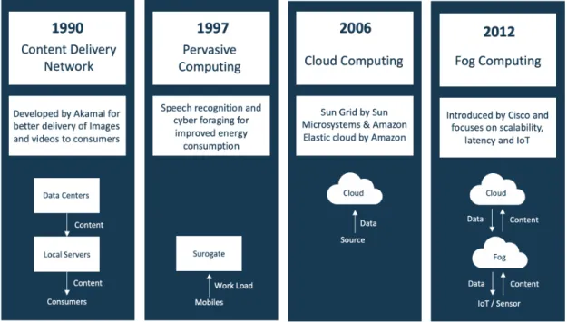
The genesis of decentralized computing can be backtracked to the 1990s when the content delivery network(CDN) was launched by Akamai, since then there have been major de-velopments in cloud computing, edge computing, IoT, and low latency Networks. When Akamai launched its content delivery network. The idea was to introduce nodes at lo-cations geographically closer to the end-user for the delivery of cached content such as images and videos.

In 1997, Akamai’s work on “Agile application-aware adaptation for mobility,” demon-strated how resource-constrained mobile devices can offload certain tasks to powerful

(11)

Figure 1. Development milestones of cloud and edge computing

servers especially for different types of applications like web browsers, graphics, video, and speech recognition (Brian D. Noble 1997) . Akamai’s work was mainly focused on pervasive computing environment as it facilitates computing and communication capabil-ities to serve users (Satyanarayanan 2001). For example, today companies like Google, Apple, and Amazon work in a similar way for speech-recognition services. The cloud computing era began in 2006 when Sun Microsystems introduced Sun Grid (later named Sun Cloud) and Amazon introduced its “Elastic Compute Cloud” (Techcrunch 2016). Amazon introduced the pay-as-you-go model (Amazon Web Services) that popularized the use of cloud computing. In telecom we did have cloud computing like solutions be-fore, early 2000s, but not as usage based payments. Amazon Web Services and other subsequent cloud providers have opened up many new opportunities in terms of com-putation, visualization, and storage capacities. However, Cloud computing comes with some security and data privacy issues and challenges, hence it is important to assess what they provide, limitations, pros, and cons and get an overall understanding of the fast-developing ecosystem (Popovi´c & Hocenski 2010).

1.2.2

Recent Developments

In 2010, Ericsson predicted that 50 billion devices would be connected by 2020, a pre-diction echoed by Cisco in 2011, as of 2018 there was an estimated 22B devices (Statista 2020). To enable such a scale of IoT devices in low latency edge computing will play an

(12)

important role. In year 2012, Edge computing started getting attention with Cisco intro-ducing fog computing for distributed cloud infrastructures (Bonomi et al. 2012). The aim was to promote IoT scalability and robustness, to handle a huge number of IoT devices and big data volumes for real-time low-latency applications. Fog computing shifts data pro-cessing to a centralized system on a local area network (LAN) by interacting with indus-trial gateways and embedded computer systems, whereas edge computing performs data processing on the compute devices directly interfacing to sensors or data origins.

To manage IoT devices, big data and to enable faster decisions, edge computing offers opportunities to take compute close to data origin, it is an ideal choice when it comes to cases with IoT devices, low latency, and real-time operations, For IoT applications to serve at the scale it is important to have the right synergy for cloud and edge. Soon, IoT solutions have to cover a much broader scope of requirements keeping scalability and robustness as the focus. As we see AI integrating into industries, it is vital to synergize edge computing and artificial intelligence to enable real-time decisions near data origins for robust and scalable systems in future.

1.3

Edge Computing

Edge Computing is the process of performing computing tasks physically close to target devices, rather than in the cloud or on the device itself (Shi et al. 2016). It enables extract-ing knowledge, insights, and makextract-ing decisions near the data origin. It is quick, secure, local, and facilitates decentralized processing. Edge computing also enables data confi-dentiality and privacy preservation on demand as it is becoming essential across multiple industries. The growing amount of data from Internet of Things (IoT) and the limitations of cloud computing (for networking, computation, and storage) currently are leading to a decentralized system like Edge Computing.

(13)

2

FRAMEWORK

In this thesis, we will implement rapid experiments for IoT and 5G set up on the edge to evaluate offloading machine learning at the edge compared to machine learning centrally at the cloud and its implications. One of the main goals of this thesis is to develop a robust and scalable operational framework for efficient continuous integration and continuous deployment of Machine learning models at the edge for AIoT applications (Wu et al. 2019). Before we delve into the experiment details, setup, and goals, let us look the benefits of using AI and machine learning at the edge in the next section.

2.1

AI and Machine Learning at the edge

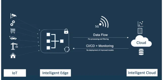
The purpose of edge computing is to put computing close to the data source and to offload centralized computing to decentralized. Edge computing makes it possible to apply differ-ent machine learning algorithms at the edge, which enable new kinds of experiences and new kinds of opportunities across many industries ranging from Mobile and Connected Home, to Security, Surveillance, and Automotive. It also enables secure and reliable per-formance for data processing and coordination of multiple devices (Beyer et al. 2018). Figure 2 depicts an overview diagram of how a secure and reliable intelligent edge archi-tecture is constructed.

(14)

Edge computing has several benefits compared to traditional cloud-based computing. For example, researchers built a service to run face recognition applications where the re-sponse time is reduced from 900 ms on the cloud to 169 ms by moving the application to edge (Yi et al. 2015). Another example where researchers used edge computing to of-fload computing tasks for wearable cognitive assistance, resulted in the improvement of response time ranging between 80 to 200 ms which is exponentially better than the central or cloud computing approach (Ha et al. 2014). Also, a by-product of this approach is the energy consumption could be reduced by 30 to 40 % by implementing edge computing (Shi et al. 2016).

The advantages for Machine Learning at the Edge are the following:

1. Stronger Hardware: In today’s world, many applications rely on very strong or spe-cialized hardware. Modern machine learning algorithms, for example, work best with GPUs or tensor processing units (TPUs). Day by day, edge devices are getting hardware upgrades that enable high computation power to small hardware devices (Girish Agarwal 2019). With upgrades and multiple edge devices, we are able to exponentially increase overall hardware capacity in order to serve and infer robust and scalable machine learning at the edge (near data origins).

2. Better Latency (compared to cloud): If applications depend on immediate feedback (e.g. to make “real-time” decisions), sending data to the cloud, calculating and sending the data back to the device may take too long. However, if the path is reduced to the (much closer) edge node and back, many use cases can be realised (Satyanarayanan 2017).

3.Hyper Personalization: Devices (IoT) can be in different environments and locations, they might need to perform tasks customised to their respective environments. in such cases edge devices or nodes can enable customisation for each device as in a custom ML model for each device performing realtime inference at close proximity (Girish Agarwal 2019). Also, this way ML models deployed at the edge can optimize and retrain when needed, constantly learn to serve better. This is limited and not possible on scale in the Cloud.

(15)

4. Data throughput: Devices may produce enormous amounts of data. One single autonomous car for example may produce up to 4000 gigabytes per day (Nelson 2016). If every single car sent all data it generates all the way to central datacenters it would create a huge load on the network. By performing the necessary computations on edge nodes close to the device, most of the paths can be pruned. This is especially important when considering the increasing importance of the internet of things and the rising number of devices connected to the internet (Shi et al. 2016).

5.Reliability and robustness: The main functionality of devices should still be available, even if communications to the central cloud are impaired. This can be achieved by relying on local communication with an Edge Node which should (in theory at least) be less prone to problems (Girish Agarwal 2019). If an edge node fails, the devices will be shifted to an alternative edge node.

6.Privacy: In many use cases collecting user data is required or useful. However, in cases where aggregated data is sufficient, the users privacy can be preserved by aggregating the data on the edge node instead of the cloud (Westerlund 2018). Edge computing can facilitate data and privacy-preserving machine learning which is also called Federated Learning (Koneˇcn`y et al. 2016), in which no edge node or centralized compute exchanges data.

7. Scalability: In most cases the computing power of devices is limited by their small size. Furthermore, developing a new use case that requires stronger hardware will require all possible users or the network administrator to update the devices, which limits the use cases adoption rate. Edge nodes do not suffer from these problems and can be extended both very easily and continuously (Beck et al. 2014). Using a suitable edge computing framework, adding, replacing or upgrading edge devices is a simple and highly automated process.

8. Adaptability: Utility of an edge node instead of a single purpose server has the added benefit of being adaptable to changing circumstances (Girish Agarwal 2019). After en-abling a base environment, edge nodes can be easily configured to provide individual sub-sets of services depending on the environment. Some use cases are only useful in cities while others may be more beneficial in rural areas. Due to the direct connection

(16)

to the cloud and higher-level Edge Nodes moving workloads and freeing up computing power for critical use cases is possible and can be done on the fly.

9.Sustainability and Cost reduction: Devices are producing enormous amounts of data. One single autonomous car for example may produce up to 4000 gigabytes per day (Nel-son 2016). If every single car sent all data it generates all the way to the cloud for machine learning inference it would create a huge load on the network and electricity consumption to serve these requests would be tremendous burden and in turn this would also result in huge costs for Businesses. Instead, outsourcing and taking Machine Learning infer-ence and data pruning at the data origin on the edge will exponentially decrease costs and enable sustainable business (Girish Agarwal 2019).

2.2

Current Problem

In this section, we will observe and reflect on some current problems, needs and trends that are leading us to envision a smarter solution to cater to future needs. Every need or growing problem presents us with opportunities to optimize and improve with the current tools. Let’s look into some trends and growing needs over the past years.

Figure 3. Growth of IoT devices over time.

source: https://www.statista.com/statistics/471264/iot-number-of-connected-devices-worldwide/

In the last decade, we have seen explosive growth in connected devices which is pioneer-ing the world into the era of Internet-of-Thpioneer-ings. Figure 3 shows how several IoT con-nected devices installed worldwide are growing in billions. To handle this growth

(17)

cloud computing has its limitations in supporting lightweight IoT devices, especially for the delay in communication context awareness of applications. These applications need to serve a high volume of IoT devices, in realtime for data processing, management of IoT networks and making context-aware decisions in realtime near the vicinity of IoT devices, this becomes necessary for paving the way to address the challenges of cloud computing and the emergence of edge computing (Ren et al. 2017). With this huge potential, some challenges would arise when we do Machine Learning on edge devices at scale to manage and monitor the machine learning models, edge devices, secure devices and their commu-nication, and efficiency of the system and many more questions around it. We can tackle these challenges by taking a systematic approach to enabling continuous deployment and continuous integration at the edge with the right synergy with the cloud. Implementing such practices in your AI projects will yield sustainable and fruitful results. You can pro-duce more productive and robust machine learning models in terms of training, execution time, deploying, and monitoring.

2.3

Solution

To address the problem of the growing number of IoT devices, big data and limitations of centralized or cloud computing, here is a birds-eye view of the process for edge and cloud synergy that will enable robust and scalable Machine Learning at the edge.

(18)

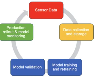
In this process, sensor data is collected from IoT device(s) by the edge device(s) where the model is inferred (ie: ML model prediction) and the collected data is concatenated with the model prediction and sent in batches for storage at the cloud. Once Data is stored successfully in the cloud, data collected in the edge is deleted.

It is a good practice to continuously monitor the incoming data and retrain your model on newer data based on the deployed machine learning model drift, if you find that the data distribution has deviated significantly from the original training data distribution (Akki-raju et al. 2018). And based on that perform retraining of the machine learning.

Model Training, Validation, and versioning are done on the cloud due to the availability of robust and scalable computation and storage enabled by cloud services. Once a machine learning model is trained or retrained it is rolled out to production deployment at the edge device(s).

We will be looking into executing this process as a solution using best-fit cloud ser-vices (from Microsoft Azure) to synergize with edge computers near IoT sensors in a low latency network to perform machine learning inference or decisions in real-time au-tonomously.

2.3.1

Research Question

The objective of the thesis is to investigate and develop methods that will enable auto-mated edge artificial intelligence. The focus of the research will be to answer the ques-tion:

"How can a framework that integrates continuous delivery and continuous deployment of machine learning models at the edge be implemented using state-of-the-art tools and methods."

2.3.2

Studies for addressing the research question

In order to address the research question we will study the following engineering areas. Following are the studies to curate an automated edge AIOps framework for AIoT appli-cation:

(19)

1. To assess the maturity of cloud services to enable operations on the edge and to identify the limitation.

2. To curate a process for continuous delivery and deployment of Machine learning models at the edge.

3. To explore ways of working in real-time IoT data processing and machine learning.

4. To observe how automated systems operate in real life and production settings.

2.3.3

Significance to the field

This thesis will contribute to the field of machine learning by exploring applied machine learning to modern technologies like edge computing, IoT, and modern networking pro-tocols (MQTT). Contribution to the field as follows,

1. Proposing a flexible architecture that can serve multiple use cases across multiple industries.

2. Assessing the current limitations of cloud services and looking at work around to achieve the most efficient ways of working for automated edge AI.

3. Validate benefits of applied machine learning at the edge such as better latency, reliability, robustness, hyper personalization, sustainability and cost reduction.

2.4

Components and processes for edge AI ecosystem

This sub-section introduces components and processes that are central to solving the re-search question.

• Edge Computing: Edge Computing allows data to be analyzed near or at the lo-cation of data origin before being sent to the cloud or data center. At the edge, knowledge can be extracted and decisions can be made using AI.

• Machine Learning: Machine learning is a method of data analysis that automates analytical model building, Machine learning algorithms can learn from data, iden-tify patterns and make decisions without much human involvement.

(20)

• Continuous Delivery and Deployment: Continuous delivery is focused on keeping software releasable all the time, continuous deployment extends it to continuously and automatically deploy new changes into production. A continuous deployment is a push-based approach, by which code changes are automatically deployed to a production environment through a pipeline as soon as they are ready, without human intervention. Continuous delivery is a pull-based approach in which a person (e.g., a manager) is required to decide which and when production-ready code changes should be released to production (Shahin et al. 2019).

• Fleet Analytics: It is aggregated analytics for each edge device used in the exper-iment which depicts device performance over a period of time with telemetry data like accelerometer, gyroscope, humidity, magnetometer, pressure and temperature. This information in turn is useful to monitor edge devices health and longevity.

• Machine Learning Lifecycle Management: Machine Learning lifecycle manage-ment is an efficient way of working for building, deploying, and managing machine learning models critical for ensuring the integrity of business processes (Raj 2019b).

• AIoT: Artificial Intelligence of Things (AIoT) is the combination of artificial intel-ligence (AI) technologies with the Internet of Things (IoT) infrastructure to achieve more efficient IoT operations, improve human-machine interactions, enhance data management, analytics and decision making (Wu et al. 2019) (Rouse 2020).

• MQTT (Networking protocol): MQTT is based on clients and brokers, were the client’s requests of receiving or sending data between each other (e.g. Edge de-vices) and broker (like a server). The broker is responsible for handling the client’s requests for receiving or sending data between each other.

1. The MQTT server is called a broker and the clients are simply the connected devices, in our case it is IoT sensors.

2. When a device (a client) wants to send data to the broker, we call this operation a “publish”. When a device (a client) wants to receive data from the broker, we call this operation a “subscribe”.

(21)

Figure 5. Schematic data flow and communication from sensor machine to edge device

MQTT is designed as a robust, session-oriented protocol especially suitable for the world of IoT, where the clientID plays the central role for session management. The MQTT specification requires the clientID to be provided within the first data frame of the protocol during session establishment. The semantics of the clientID is to provide the unique way a session can be (re)established between a client and the broker, without any further information. So the clientID is required to be unique per broker over time, hence, no collision of clientIDs should ever happen. As the clients are not aware of each other, but usually provide their own clientID, it must be drawn from large set of possible clientIDs so the probability of a collision of clientIDs is negligible.

2.5

Limitations

Edge computing has many advantages (as discussed in section 2.1), but also has certain limitations. Some limitations of edge computing are shown in figure 6 .

(22)

Figure 6. Limitations of edge computing.

1. More Hardware: Edge computing requires setting up more local hardware. Eg: IoT cameras on the street or self driving cars require a built-in compute hardware to process, infer and send video data over the internet to the cloud as well as a more sophisticated computing process for more advance process applications, such as objects-detection, motion-detection or facial-recognition algorithm. So for adop-tion of edge computing on scale a massive add on to existing infrastructure is needed in terms of more computing power.

2. Data limitations: Edge devices store, processes and analyzes only a subset of data, discarding raw information and sending only needed information to the cloud. Or-ganizations must consider what level of loss of data is acceptable and have a solid data strategy in place for edge computing. Contrary to this data pruning when done right can be a major benefit. Edge devices also have limited access to full data in cloud or on-sight and it’s data governance is limited to edge device only.

3. Security: Edge computing can increase the probability of attacks. With IoT sensors, networking, and built-in computing the chances of attacks by malicious hackers to infiltrate the devices and access sensitive data have increased. One potential risk is data and device manipulation attacks. If hacked, it is possible to manipulate the device about the data it has collected, leading to bad decisions. Security is an important area in edge computing, in most of the use cases privacy and compliance are highly important so edge-cloud setup has to comply with data privacy and laws for location (Beck et al. 2014).

(23)

2.6

Aim of the project

The aim of the project is to evaluate, validate or develop a robust and scalable framework for edge computing that will enable automated machine learning at the edge for AIOT ap-plications, The application will be fairly industry and use case agnostic. This framework would facilitate:

• Continuous integration and continuous deployment of Machine Learning models at the edge.

• Fleet analytics to monitor edge devices in real-time.

(24)

3

RESEARCH THEORY AND METHODOLOGY

Studies in software engineering are often of an interdisciplinary nature and this thesis is not an exception. The research field of software engineering is often defined as an intersection of information technology, business, and data processing. In this study, the business dimension is focused on private and public companies determined to optimize re-sources, increase efficiency and upgrade their existing services to be smarter and enabled by the power of artificial intelligence through real time data using Internet-of-Things. For the social context of the research these businesses have goals to optimize resources in terms of energy, time, money and human resources. Optimizing these resources will drive efficiency, growth and adoption of modern technologies like edge computing, artificial intelligence of things (AIoT) and low latency networks.

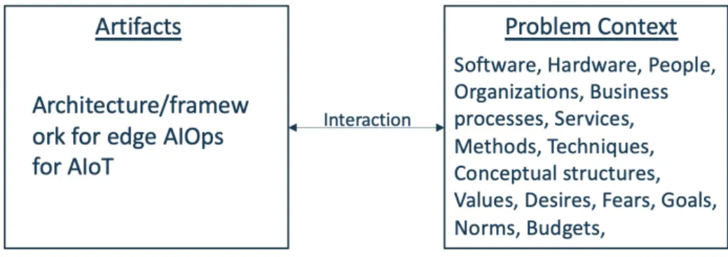
In order to address our research question we will follow a design science method pro-posed by Wieringa (2014). Design science is the design and investigation of artifacts in a context. The artifacts we study are designed to interact with a problem context in order to improve something in that context.

Figure 7. The subject of design science: an artifact interacting with a context

In our case the artifact in context will be the edge MLOps framework for AIoT appli-cations that we will design iteratively while interacting with the problem context which boils down to our project or experiments we perform in order to evaluate and validate the scalability and robustness of the artifact in the context. The project and experiments we will work on replicates software, hardware, people, organizations, business processes, services and values of the real world setup with similar social context as discussed above (VTT 2019).

(25)

3.1

Towards a Research Methodology using Design

Sci-ence

The research method used follows the outline of design science. In a structured and itera-tive approach, we implement two cycles (Design cycle and Empirical cycle) for qualitaitera-tive and quantitative analysis and conclusions for our design solution.

3.1.1

Design Cycle

Design problems call for a change in the real world and require an analysis of actual or hypothetical stakeholder goals. A solution is a design, and there are usually many different solutions. There may even be as many solutions as there are designers. These are evaluated by their utility with respect to the stakeholder goals, and there is not one single best solution. For example, what is an accurate algorithm for image classification? there isn’t a one go to solution for image classification but instead there are different algorithms, designs and ways of classification. It is about finding the right algorithm or way of working for the current problem. We can have an ideal design to address a problem context but not a one and the only design. Ideal design to solve a problem in a generalized approach is achieved by iterative experiments on problem to find ideal solution by assessing the utility value for the problem context.

To design an ideal workflow or ecosystem for our problem context (AIoT on edge com-puting) its application and utility will be industry and use case agnostic. This will be achieved by exploring and building through services available on a popular cloud service Microsoft Azure. This ecosystem would facilitate,

• CI/CD of Machine Learning models at the edge

• Fleet Analytics

• Machine learning model lifecycle management

To iterate in design cycle we will work on the following problem context (experiment): Predict room air quality for anomaly detection using Machine Learning on the edge. Ex-periment setup has 3 rooms with an edge computer in each (3 edge computers in total) upon receiving data from sensors, edge devices should make machine learning model

(26)

in-ference to predict air quality in next 15 minutes, this process or flow has to be automated using state-of-the-art tools and methods.

3.1.2

Empirical Cycle

Empirical cycle which is a rational way to answer scientific knowledge questions. It is structured approach for qualitative and quantitative analysis and conclusions for our design solution.

Below is a set of question in form of a checklist to decide the success of our design solution. Goal is to get the optimal results in an iterative process.

1. Research problem analysis: To investigate an improvement of problem in the field.

• To explore ways of working in real-time with IoT data processing and machine learning.

• To explore methods for applied machine learning for real-time multivariate time series forecasting.

• To observe how automated systems operate in real life and production settings.

2. Research design and inference design: To survey possible methods.

• To assess the maturity of cloud services to enable operations on the edge and to identify the limitation.

• To curate a process for Continuous delivery and deployment of Machine learn-ing models at the edge

• Machine Learning lifecycle management design for edge AI.

3. Validation of research and inference design:

• Robustness: Stability of CI/CD pipeline (Number of successful triggers) for cloud to edge, Stability of CI for IoT devices to edge devices, Hardware compatibility, Model performance (number of models changed, model drifts), models retrained (Success and failed), fleet analytics and data storage.

(27)

• Scalabilty: Number of Devices, Multiple Cloud, Network scaling.

• Application: Industries and use cases agnosticity.

• Resources Optimization: Optimization of Energy, Time, Human interaction and Cost compared to cloud computing (current setup).

3.2

Applied Machine Learning Methods

We look at the problem of predicting a single variable (future air quality - 15 minutes in the future) using multiple independent variables. In this section we explore the Machine Learning methods applied on the data to develop models that will be deployed on the edge devices to make real-time prediction. Let’s look at them one by one.

1. Multiple Linear Regression (MLR)

Multiple linear regression, models the relationship between two or more explanatory vari-ables in correlation to a response variable. In order to understand the correlation better, we segregate all the variables into two categories namely, independent variables and de-pendent variable

INDEPENDENT VARIABLES (X) : Variables or factors which are used to correlate to

re-sponse or prediction or dependent variable.

DEPENDENT VARIABLES(Y): The outcome variable is called the dependent variable.

Every value of the independent variable x is associated with a value of the dependent variable y (Preacher et al. 2006). The correlation between the independent and dependent variables is calibrated by a regression line in an n-dimensional space for all independent variables. let’s say there are n independent variables x1, x2, ... , xn. To predict y or the independent variable, correlation is defined to be

(28)

This line describes how the mean response y changes with the independent variables. The observed values for y vary about their means y and are assumed to have the same standard deviation. The coefficients

β0,β1,β2,β3, ....βn (2)

are fitted or calibrated to estimate the parameters 0, 1, ..., n of the regression line in order to predict the independent variable y.

2. Extreme Learning Machines

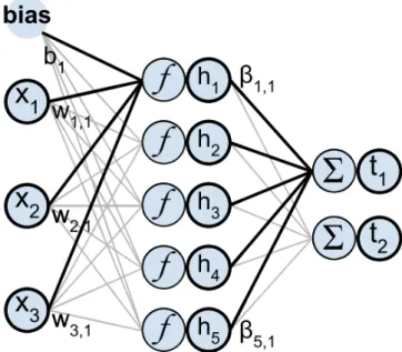
The extreme learning machine has demonstrated excellent performance in a variety of ma-chine learning tasks including situations with missing values. Extreme learning mama-chine is a single layer feedforward neural network with randomly generated neurons for regres-sion, classification, clustering, sparse approximation, compresregres-sion, and feature learning (Akusok et al. 2015). In most cases, the output weights of hidden nodes are usually learned in a single step, which essentially amounts to learning a linear model.

Figure 8. Computing the output of an SLFN (ELM) model Printed with permission from author Anton Akusok (Akusok et al. 2015).

A hidden layer randomly generates loosely correlated hidden layer features, it allows for a solution with a small normalization and a good generalized performance.

(29)

A mathematical description of an ELM is as following. Consider a set of N distinct training samples(xi,ti), i∈[[1, N]] withxi∈Rd andti∈Rc. Then a single hidden layer feed forward network with L hidden neurons has the following output equation:

L

∑

j=1

βjφ(wjxi+bj),i∈[1,N] (3)

with φ being the activation function, Sigmoid function is a common choice, but other activation functions are also possible like linear, tan-sigmoid, sin etc (Huang et al. 2011) (Huang 2014) (Huang 2015).w_ithe input weights,b_ithe biases andβithe output weights. The relation between inputs xi of the network, target outputsti and estimated outputs yi is: yj= L

∑

j=1 βjφ(wjxi+bj) =ti+∈i,i∈[1,N], (4)

where∈is noise. Here the noise includes both random noises and dependency on vari-ables not presented in the inputs X (Akusok et al. 2015).

3. Random Forest Regressor Random forest is a type of ensemble learning with the use of multiple decision trees and a technique called Bootstrap Aggregation, commonly known as bagging (Segal 2004). Ensemble Learning is when you take multiple algo-rithms, combine their output to archive a better combined result than the original (Zhang & Ma 2012).

(30)

Figure 9. Random forest structure

Random forest is a bagging technique. There is no interaction between these trees while building the trees. The trees in random forests are run in parallel (Liaw et al. 2002).

These are the steps to build a random forest regressor

• Step 1: Pick k random points from the training dataset.

• Step 2: Build the decision trees associated with these K data points.

• Step 3: Choose N number of trees you want to build and repeat steps 1 and 2.

• Step 4: For the new data point or test input, make each one of your N trees predict the value of y for the data point in question, and assign the new data point the average across all of the predicted y values.

Let’s say y is the dependent variable to predict and x1, x2, x3 .... xn are independent variables, then we predict y by making each of N number of trees predict the value of y and then average all predictions to derive final prediction for y.

ˆ y= 1 n n

∑

i=1 y_i=y1+y2+· · ·+yn n (5)

(31)

4. Support Vector Regressor

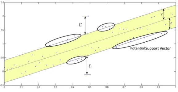
The regression problem is a generalization of classification problem, in which the model returns a continuous-valued output, as opposed to an output from a finite set (Ratkowsky & Giles 1990). In other words, a regression model estimates a continuous-valued multi-variate function. SVMs solve binary classification problems by formulating them as con-vex optimization problems. The optimization problem entails finding the maximum mar-gin separating the hyperplane, while correctly classifying as many training points as pos-sible. SVMs represent this optimal hyperplane with support vectors (Drucker et al. 1997). The sparse solution and good generalization of the SVM lend themselves to the adaptation to regression problems. SVM generalization to SVR is accomplished by introducing an ε-insensitive region around the function, called theε-tube. This tube reformulates the op-timization problem to find the tube that best approximates the continuous-valued function while balancing model complexity and prediction error. More specifically, SVR is for-mulated as an optimization problem by first defining a convexε-insensitive loss function to be minimized and finding the flattest tube that contains most of the training instances. Hence, a multiobjective function is constructed from the loss function and the geometrical properties of the tube.

Then, the convex optimization, which has a unique solution, is solved, using appropriate numerical optimization algorithms. The hyperplane is represented in terms of support vectors, which are training samples that lie outside the boundary of the tube. As in SVM, the support vectors in SVR are the most influential instances that affect the shape of the tube, and the training and test data are assumed to be independent and identically distributed, drawn from the same fixed but unknown probability distribution function in a supervised-learning context (Gunn et al. 1998).

(32)

Figure 10. One-dimensional linear SVR

This is a one-dimensional view of an optimized ε-insensitive tube for data points with potential support vectors. εi andε∗_i are the slack variables withεi being variables repre-senting training data points above theεinsensitive tube andε∗_i is for data points belowε insensitive tube. 1 2||ω|| 2₊_C m

∑

i−1 (εi−ε∗i)→min (6)

SVR formulates this function approximation problem as an optimization problem that attempts to find the narrowest tube centered around the surface while minimizing the pre-diction error, that is, the distance between the predicted and the desired outputs. The former condition produces the objective function, where ||ω|| is the magnitude of the nor-mal vector to the surface that is being approximated.

(33)

4

EXPERIMENTS

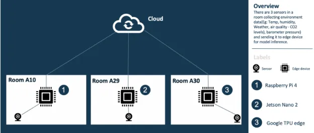
The study is performed through a collaboration project - Smart Otaniemi together with Ti-etoEvry (industry partner) and VTT Finland (research partner). To perform experiments for the thesis, there was a need for infrastructure (IoT and 5G) and a platform to exper-iment with AI on the edge and IoT devices in real-time. Partners provisioned needed infrastructure and platform to perform experiments in VTT’s 5G campus in Helsinki, Fin-land.

4.1

Setup

At the 5G campus, there are 26 rooms with 26 IoT devices monitoring room air quality and conditions 24x7. Each sensor collects and sends data to the central network/database or station on an interval of 5 minutes.

In the execution of the experiment for the thesis, we narrowed it down to three rooms as shown below in figure 11. The reason for selecting these rooms is described in the Data Analysis section.

(34)

4.1.1

Hardware Tools

In order to implement this setup, following hardware is used for edge computers:

• NVIDIA Jetson Nano2: https://www.nvidia.com/jetson-nano/

• Google TPU edge: https://cloud.google.com/edge-tpu/

• Raspberry Pi 4: https://www.raspberrypi.org/products/raspberry-pi-4-model-b/

Raspberry Pi 4 was setup in room A10, Nvidia Jetson Nano 2 was setup in room A29 and Google TPU edge was setup in room A30. Detailed steps of setup and installation for each device listed in Appendix A.

4.1.2

Software Tools

For software development, I have chosen these common data scientist’s tools for the tech stack to do data analysis, model training and deployment, and monitoring - python, linux, and docker. The programming language used to conduct experiments for this thesis is Python (version 3.6.7). Numerous libraries are used for different purposes to assist exper-iments. Find the list of the major libraries used in Appendix B.

For Deployments - Docker containers are used to deploy applications in runtime, a docker container image is a lightweight, standalone, executable package of software that includes everything needed to run an application: code, runtime, system tools, system libraries and settings. For cloud - Microsoft Azure is used. Microsoft Azure is a cloud computing ser-vice created by Microsoft for building, testing, deploying, and managing applications and services through Microsoft-managed data centers. All of these computer systems, middle-ware and services need to be arranged and coordinated in such a way that they automated multiple tasks and systems, this process is called as orchestration. Orchestration takes advantage of multiple tasks that are automated to automatically execute a larger workflow or process. The goal of orchestration is to streamline frequent and repeatable processes to ensure optimization and efficient deployment of software. To achieve efficient edge and cloud synergy, services from Azure cloud are used to orchestrate edge to cloud operations for continuous delivery and deployment.

(35)

4.2

Machine Learning Operations for AIoT Application

This section describes the systematic approach to Machine Learning operations (MLOps) for data collection, exploratory data analysis, feature extraction and machine learning models training done before our experiments for AIoT applications in real-time. To train we need computation and storage resources and on top of that a platform to train the ma-chine learning models. For this purpose we use Azure Mama-chine Learning service as a platform where we can provision compute, storage and needed infrastructure on request. It is a framework providing an end-to-end solution for machine learning model develop-ment as follows:

• Resource provisioning

• Data versioning

• Model training

• Model storing and versioning

• Model packetizing

• Model deploying

• Monitoring

With these features we will be able to train, manage, deploy and audit models (model traceability for data and source code used to train). Models are trained separately to be deployed in respective rooms and edge devices.

4.2.1

Dataset Analysis

This section describes the data that will be used in the experiments to train the machine learning models to be deployed in the edge devices to carry out the experiment and eval-uate. The data has been collected for 3 months, starting from 15th October 2019 to 15th January 2020 from 26 different IoT devices.

(36)

4.2.1.1 Data descriptors - Here are the data descriptors for data collected from IoT devices.

1. timestamp - Time of data (datetime) 2. name - Name of sensor (str)

3. room - The room where sensor is placed or data origin (str) 4. room type - Type of room (str)

5. floor - Floor where data was generated (str) 6. air quality - Air quality index altered (float)

7. air quality static - Air quality index unaltered (float) 8. ambient light - Light present in the room (float) 9. humidity - Humidity in the room (float)

10. iaq accuracy - Indoor Air Quality accuracy altered (float)

11. iaq accuracy static - Indoor air quality accuracy un altered (float) 12. pressure - Pressure in the room (float)

13. temperature - Temperature in the room (float)

• air quality and air quality static: Air quality and air quality Static are air quality indexes in the room ranging from 0 to 250. Air quality static is raw sensor reading and air quality is augmented data. Air quality is hazardous for humans in the range 150-250 (Coway 2016). Air quality is augmented data of air quality static. air quality static is the raw reading for IoT device sensors.

• ambient light: Ambient light is the measurement of ambient light intensity that matches the human eye’s response to light under a variety of lighting conditions.

• humidity: Humidity measures and reports both moisture and air temperature. The ratio of moisture in the air to the highest amount of moisture at a particular air temperature is called relative humidity. Units measured by the sensor are grams per cubic meter. Humidity ranges from 0 to 50, anything above 40 grams per cubic meter can be uneasy for human activity in the room.

• iaq accuracy and iaq accuracy static: One of the factors to calibrate indoor air quality (IAQ) is iaq accuracy. IAQ Accuracy=1 means the background history of the sensor is uncertain. This typically means the gas sensor data was too stable to clearly define its references, IAQ Accuracy=2 means sensor found a new calibration data and is currently calibrating, IAQ Accuracy=3 means data calibrated success-fully. IAQ accuracy is augmented data and iaq accuracy static is the raw reading for

(37)

IoT device sensors.

• pressure: Pressure in the room is measured in kpa ranging from 0 to 1040.

• temperature: Temperatures in the room have been measure between 0-26◦c.

Here is a snapshot of the raw data collected from IoT devices.

Figure 12. Data snapshot of 3 months of data collected from IoT sensors

Here is an overview of the data collected from IoT devices,

• Timeline - 3 months (15-10-2019 to 15-01-2019)

• Total 537873 number of rows or events were recorded.

• Size of the data: 45.9 MB.

Each IoT device generated an event or recorded data at a time interval of 5 mins which equals to 12 events in an hours.

4.2.1.2 Stationarity analysis After assessing time series of air quality for each room’s data, figure 13 shows non-stationary pattern since mean, variance and covariance are ob-served to be changing over time. Non-stationary behaviors can be trends, cycles, random walks or combinations of the three as observed in figure 13.

(38)

Figure 13. Data non-stationarity over time observed for selected rooms.

There are 26 rooms, each room has an IoT device to monitor room conditions. Over the period in which data was collected, each room has around 46000 events recorded as shown in figure 14.

Figure 14. Frequency of data in each room.

There are three types of rooms in the premises, most of them are being office rooms. Rest are meeting rooms and corridor rooms. Here is the collective data frequency for each type of room described in figure 15.

(39)

Figure 15. Frequency of data in each room.

After the data analysis, we narrowed down the experiment to only 3 different rooms. Reason being we wanted to experiment on meeting rooms, since we had only 2 meet-ing rooms available, they were chosen. And one office room was chosen with highest frequency of unhealthy air quality. These are the selected rooms: room_a10, room_a29, room_a30.

Here is the normal distribution of air quality in selected rooms as shown in figure 16.

(40)

Table 1. Descriptive statistics for air quality in selected rooms. Selected Rooms

Room name Room type Unhealthy air

quality frequency

Avg. air quality

Room A10 Office room 2033 61.92

Room A29 Meeting Room 2205 61.40

Room A30 Meeting Room 1085 55.45

Descriptive statistics for rooms are listed in table 1 with unhealthy air quality frequency and Avg. air quality for each room.

4.2.1.3 Empirical data analysis for selected rooms In order to assess room condi-tions and anomalous behavior. Let us look at data in detail for each room in this order room a10, room a29 and room a30.

1. Room a10 - Office room

Figure 17. Emprical analysis for room a10.

Histograms for all columns in the data for room a10 are generated (in figure 17) to get a holistic view of data and observe overall conditions and anomalies.

(41)

For both, the majority of data points for air quality and air quality static range in good air quality (ie: 0-100) which is a good sign as it shows quality of the air in the room is good majority of the time. Quality of the air is also observed to have some anomalies or worse (ie: 150-250) on some occasions, this range is hazardous for humans in the room (Coway 2016). Ambient light is in two extremes either 1 or 25-30. Average humidity in the room is observed to be in the range 25-35 grams per cubic meter which is healthy for humans, anything above 40 grams per cubic meter can be uneasy for human activity in the room. IAQ accuracy is mostly 1 with some cases of 3 and very few samples of 2. In most cases, the pressure is between the range 990 to 1020. The majority of data points for temperature are ranging in 21-24◦C which is optimal room temperature. Some anomalies have been observed with low temperatures as below 10◦C and above 25◦C. In figure 18, a time-series sensor data for room a10 data progression over time can be observed in these graphs.

Figure 18. Timeseries data progression for room a10

Air quality and air quality static have identical progressions of data over time and the data is non-stationary. Likewise, humidity, pressure and temperature are observed to be non-stationary and independent of each other.

(42)

Some anomalies and peaks are noticeable for ambient light, IAQ accuracy and IAQ ac-curacy static. For our experiment, we predict air quality static using machine learning at the edge devices. Figure 13 shows how air quality static has progressed over time. Some anomalies and peaks have been noticed for the timeline of 25-10-2019 to 01-11-2019, 01-12-209 to 7-12-2019 and 28-12-2019 to 10-01-2020. Upon cross-checking with the premises authorities they have validated these peaks to be the busiest time during this time of the year where they have a high amount of human activity, i.e. meetings in our case for room a10. These peaks in data are useful for our machine learning models to learn and predict. The average air quality in room_a10 is 61.92.

2. Room a29 - Meeting room

Figure 19. Emprical analysis for room a29

To get a holistic view of data and observe overall conditions and anomalies, histograms are generated for all columns in the data for meeting room a29 (in figure 19). For both air quality and air quality static, the majority of data points range in good air quality (ie: 0-100) which is a good sign as it shows air quality in the room is a good majority of the time. In few instances both are observed to have some anomalies or worse (ie: 150-250), this range is hazardous for humans in the room. Ambient light is in two extremes either

(43)

In many instances humidity is observed to be in the range of 25-35 grams per cubic meter which is healthy for humans. IAQ accuracy is mostly 1 with some cases of 3 similar to room_a10. Data observed in the histograms shows IAQ accuracy and IAQ accuracy static are identical. In most events pressure is between the range 1000 to 1020 kpa. In most of the instances, the temperature is ranging between 21-24◦C. Some anomalies have been observed now and then with low temperatures as below 10◦C and above 25◦C. In figure 20, a time-series sensor data for room_a29 data progression over time can be observed in these graphs.

The data is non-stationary, air quality and air quality static have an identical progression over time. Humidity, pressure and temperature are observed to be non-stationary and in-dependent of each other. From Figure 13 we observe that air quality static has progressed over time and some anomalies and peaks have been noticed for the timeline of 25-10-2019 to 01-11-2019, 01-12-209 to 7-12-2019 and 28-12-2019 to 10-01-2020. These peaks in data are useful for our machine learning models to learn and predict. The average air quality in room_a29 is 61.40.

(44)

3. Room a30 - Meeting room

Like above rooms histograms for all columns in the data for meeting room room a30 are generated (in figure 21)

Figure 21. Emprical analysis for room a30

Air quality and air quality Static mostly happen to in good range (i.e.: 0-100) Some anomalies observed (ie: 150-250) on some occasions (Coway 2016). Ambient light is in two extremes either 1-9 or 60-80. Most of the humidity ranges from 25-40 grams per cubic meter which is healthy for humans. IAQ and iaq accuracy static are observed to be 1 for all instances. The pressure is mostly distributed in range 990 to 1020. Temperatures in the room are observed to be optimal mostly.

(45)

In figure 22, a time-series sensor data for room_a30 data progression over time can be observed in these graphs. Some anomalies and peaks are noticeable for ambient light, IAQ accuracy and IAQ accuracy static. Air quality and air quality static have identical progression of data over time and the data is non-stationary. Likewise humidity, pressure and temperature are observed to be non-stationary and independent to each other. Some anomalies and peaks for air quality have been noticed in Figure 13 for timeline of 11-01-2019 to 12-11-11-01-2019 and 01-12-209 to 10-12-11-01-2019.

4.2.2

Feature Engineering

Feature engineering is transforming raw data into meaningful features so that data can be better represented and prepared for predictive modeling (Severyn & Moschitti 2013). As a result model accuracy is improved on unseen data. This section describes feature engineering on the data. Feature engineering steps involved feature extraction, correlation and scaling to prepare data for machine learning model training. Let us look into each step.

(46)

4.2.2.1 Feature Extraction After exploring data and identifying patterns in the above section, we clearly see important data parameters or columns that correlate to the air quality inside a room. Based on the data analysis, these are the parameters or columns that we will choose for training machine learning algorithms to predict air quality inside a room after 15 minutes.

1. air quality static 2. ambient light 3. humidity

4. iaq accuracy static 5. pressure

6. temperature

In order to predict air quality 15 minutes ahead, a new feature is created "future air qual-ity" which is 15 minutes ahead of the current event, this feature is created by shifting the column "air quality static" three rows ahead. As each row or event in air quality static is created at 5 minutes interval, shifting it 3 rows ahead to create a new column will give us a column named "future air quality" which has 15 mins ahead air quality for given air quality static. After selecting needed columns and creating needed features, here is a snapshot of data in figure 23.

(47)

4.2.2.2 Feature Correlation Data and feature correlation is an important step in the feature selection for machine learning model training, especially when the data type for the features is continuous, as it is in our case. Pearson Correlation Coefficient can be used with continuous variables that have a linear relationship (Benesty et al. 2009). To under-stand the relationship, we observed data and feature correlation between the variable to predict and other attributes in the data. For the feature "future_air_quality" we calculated feature scores using Pearson correlation.

Figure 24. Feature correlation using pearson correlation.

We observed patterns for each room for our experiment as shown in figure 24. The fea-ture "fufea-ture_air_quality" shows a positive correlation with air_quality_static, pressure, ambient_light and iaq_accuracy to some extent. Positive correlation implies that feature A increases then feature B also increases or if feature A decreases then feature B also decreases. Both features have a linear relationship and move in tandem. In figure 24 we see a strong positive correlation for feature future_air_quality to air_quality_static and pressure. Humidity has a strong negative correlation which implies if feature A increases then feature B decreases and vice versa.

(48)

4.2.2.3 Feature Scaling The next step is to do feature scaling in order to get the data ready for Machine Learning training.

Feature Scaling is a technique to standardize the independent features present in the data in a fixed range. It is performed during the data pre-processing to handle highly varying magnitudes or values or units. If feature scaling is not done, then a machine learning algorithm tends to weigh greater values, higher and consider smaller values as the lower values, regardless of the unit of the values.

We perform standardization technique for feature scaling, in formal terms it is defined as

X_new= Xi−Xmean

standardDeviation (7)

It re-scales a feature value so that it has distribution with 0 mean value and variance equals to 1. With this we are ready for machine learning training with our new features and scaled data.

4.2.3

Model Training

In this section we will assess machine learning models trained to predict air quality based on variables we engineered in section 4.3. Below are the variables after feature engineer-ing (that will be input to the model to predict future air quality).

• air quality static

• ambient light

• humidity

• iaq accuracy static

• pressure

• temperature

• future air quality

From the above variables we domultivariate time series predictionto predict future air quality 15 minutes after current time inside a particular room. These are the algorithms trained for data (section 4) for each room respectively (Each algorithm explained in detail in section 4.4)

(49)

1. Multiple Linear Regression (MLR)

2. Extreme Learning Machines (ELM)

3. Random forest Regressor (RFR)

4. Support Vector Regressor (SVR)

We performed cross validation using Timeseries Split as explained below to train and evaluate models.

4.2.3.1 Cross Validation - Timeseries Split In time series machine learning analysis, our observations are not independent but time dependent, so we cannot split the data randomly as we do in non-time-series analysis (Eg: Train, validation and test). Instead, we split observations along with the sequences.

Training data is split into multiple segments (10 segments for our experiment). We use the first segment to train the model with a set of hyper-parameter, to test it with the second. Then we train the model with first two chunks and measure it with the third part of the data. In this way we do k-1 times of cross-validation.

Figure 25. Timeseries split - Cross validation

For model training for our experiment timeseries split was implemented with 10 splits (using scikit-learn library).

(50)

4.2.4

Model Evaluation

We evaluate trained models using Timeseries split (cross validation) and root mean square error (RMSE) for metrics.

4.2.4.1 Metrics In order to assess model training performance Root Mean Square Error (RMSE)is used as it is a standard way to measure the error of a model in predicting quantitative data. Formally it is defined as,

RMSE=

r

∑(yt−yp)2

n (8)

yp1,yp2,yp3...ypn are predicted values by the model. yt1,yt2,yt3...ytn are the obe-served values. n is the number of observations.

To calibrate final results for trained models performance Timeseries split (10 fold cross-validation) was implemented to take the average of RMSE of each fold. Also, trained models were tested on test data which is 20% of the total data for each respective room. Detailed results can be observed in table 2 for trained models on the data for respective rooms after Timeseries split (10-fold cross-validation), hyperparameter tuning and grid searching for best parameters for each algorithm.

After assessing the performance of each model on 10 fold cross-validation (Timeseries Split) and test data (20% of training data). Here is the ranking of model performance after model training in ascending order,

1. Multiple Linear Regression (MLR) 2. Support Vector Regressor (SVR) 3. Extreme Learning Machines (ELM) 4. Random forest Regressor (RFR)

(51)

Table 2. Model training results.

Model Training Results

Room name Algorithm Cross Validation RMSE (train)

Test RMSE

Room A10 MLR 5.020 5.875

Room A10 ELM 6.325 6.208

Room A10 RFR 10.710 9.987

Room A10 SVR 6.046 5.977

Room A29 MLR 5.362 4.158

Room A29 ELM 11.202 4.223

Room A29 RFR 11.676 9.208

Room A29 SVR 8.073 4.176

Room A30 MLR 3.648 3.551

Room A30 ELM 7.920 3.895

Room A30 RFR 9.686 7.720

Room A30 SVR 5.177 3.55

4.2.5

Model Packaging

To do machine learning inference at the edge we have to serialize and package needed ar-tifacts and machine learning models. Following are the arar-tifacts serialized to be exported to production environments,

4.2.5.1 Input and output scaler : We performed a standardization technique for fea-ture scaling. It re-scales a feafea-ture value so that it has distribution with 0 mean value and variance equals to 1. Similarly, we have to scale incoming input data for model inference to be able to predict future air quality 15 minutes in the future. For this purpose, the feature scaling variable is serialized to a pickle file (.pkl).

4.2.5.2 Machine learning models : All trained and retrained ML models are serial-ized in the Open Neural Network Exchange (ONNX) format. ONNX is an open ecosys-tem for interoperable AI models, it enables model interoperability and serialization of ML and deep learning models in a standard format (.onnx). With this, all trained or retrained models and artifacts are ready to be exported and deployed to production envi-ronments.

4.3

Design Cycle: Proposed framework for Edge MLOps

In this section we design a framework for edge MLOps, we start by assessing For edge and cloud communication to be robust and realtime, it is essential to assess every

(52)

ser-vice provided by the cloud serser-vice to make an efficient synergy between edge and cloud. There is a range of services Azure offers to facilitate edge-cloud operations. We assessed some services on Microsoft Azure with a goal to facilitate continuous delivery, deploy-ment and monitoring on edge devices, to orchestrate cl