Binary Partition Tree as an Efficient Representation
for Image Processing, Segmentation, and Information
Retrieval
Philippe Salembier, Member, IEEE, and Luis Garrido
Abstract—This paper discusses the interest of Binary Parti-tion Trees as a region-oriented image representaParti-tion. Binary
Partition Trees concentrate in a compact and structured rep-resentation a set of meaningful regions that can be extracted from an image. They offer a multi-scale representation of the image and define a translation invariant 2-connectivity rule among regions. As shown in the paper, this representa-tion can be used for a large number of processing goals such as filtering, segmentation, information retrieval and visual browsing. Furthermore, the processing of the tree represen-tation leads to very efficient algorithms. Finally, for some applications, it may be interesting to compute the Binary Partition Tree once and to store it for subsequent use for various applications. In this context, the last section of the paper will show that the amount of bits necessary to encode a Binary Partition Tree remains moderate.
Keywords— Nonlinear filtering, Connected operators,
Mathematical morphology, Segmentation, Partition tree, Region Adjacency Graphs, Pruning strategy, Object recog-nition, Browsing, Information retrieval.
I. INTRODUCTION
A
N INCREASING number of image processing application-s rely on application-some type of region-baapplication-sed repreapplication-sentationapplication-s of im-ages. The traditional image representation involving a rectan-gular array of pixels has major drawbacks. Its elementary unit, the pixel, provides an extremely local information. As a result, image processing at the pixel level has to face major difficulties in terms of scale: the scale of representation is most of the time far too low with respect to the interpretation or decision scale. Another drawback of pixel-based representation is the number of pixels. Most of the time, algorithms working at the pixel level are restricted to be very simple because they have to deal with a very large number of pixels.
Region-based representation of images potentially offers an attractive solution to this problem: the representation can be ac-curate; it involves a number of regions that is much lower than the number of original pixels and it can be considered as a first level of abstraction with regard to the raw information. Most
Manuscript received July 17, 1998; revised September 8, 1999. This work was supported in part by France-Telecom/CCETT under contract 96ME22. The associate editor coordinating the review of this manuscript and approving it for publication was prof. Glenn Healey.
The Authors are with the Universitat Polit`ecnica de Catalunya, Barcelona, Spain (e-mail: [email protected]).
Publisher Item Identifier S 1057-7149(00)02678-6.
of the time, region-based representations are created by merg-ing similar pixels and by structurmerg-ing the resultmerg-ing regions within a Region Adjacency Graph (RAG). Even if some contribution-s have been publicontribution-shed in the pacontribution-st about image procecontribution-scontribution-sing on RAGs, it has to be recognized that they are not widely used in practice.
For practical applications, RAGs have two main drawbacks: They just describe one scale of the image and the connectivity between regions is not space invariant. In this paper, we propose a region-based representation called Binary Partition Tree that addresses these two drawback of RAGs. Binary Partition Trees represent images at various scales and the connectivity between regions is translation invariant since the tree encodes the relation between each region and only one of its neighboring regions. It is a 2-connectivity rule.
This study about Binary Partition Trees is related to several fields of image processing where region-based representation of images have proved to be useful: Filtering strategies involving connected operators, segmentation algorithms and content de-scription.
Connected operators: These filtering tools [17], [5], [16]
are derived from mathematical morphology. They interac-t wiinterac-th interac-the signal by means of specific regions called flainterac-t
zones (largest connected components of the space where
the image is constant). A connected operator is an oper-ator that only merges flat zones. As it cannot introduce any new contour, it simplifies as well as preserves the con-tour information. The theory and applications of connect-ed operators are rapidly progressing [19], [21], [18], [1], [4], [8]. However, one of the major drawbacks of classi-cal operators is that they consider that objects composing the scene are either bright or dark image components (as a result, they simplify either bright or dark objects). This very crude assumption limits their usefulness for certain applications. In this paper, we discuss the interest of Bina-ry Partition Trees to create new connected operators that do not suffer from this restriction.
Segmentation: A large number of segmentation techniques
such as region growing or watershed rely on iterative merging strategies [2], [10], [9]. These algorithms sequen-tially merge either pixels or regions. In practice, the class of rules used to control the merging process is restricted. Indeed, rules involving the global optimization of a cri-terion that has no specific property (such as increasing-ness) are not straightforward to deal with. In such cases, it is difficult to know, at a given time instant, if a particu-lar merging will eventually lead to the optimization of the
global criterion and, for practical reasons, it is generally not realistic to memorize and to keep track of all merging possibilities so that they can be undone in future steps. Recently, a study on the class of merging techniques has shown that a large set of interesting operators can be viewed either as filtering tools or as segmentation algo-rithms [7]. The definition of this class of operators relies on three notions:
1. merging order defines the notion of region homogene-ity;
2. merging criterion characterizes the set of regions we are interested in;
3. region model defines how regions are represented. In a large number of classical segmentation algorithms, the notions of merging order and merging criterion are com-bined into what is called the segmentation criterion. As will be seen in this paper, Binary Partition Trees strong-ly restrong-ly on a clear separation between merging order and merging criterion.
Content description: There is currently a strong interest in
defining content descriptor for information retrieval (activ-ities within the MPEG-7 forum for example). If we con-sider a low level descriptor such as color or shape, one of the first issues to be faced is the selection of the scale at which the description has to be done. Since the queries done during the retrieval may deal with very different s-cales, it is not pertinent to a priori fix the description scale. As a result, a color (shape) descriptor should be able to de-scribe the color (shapes) at multiple levels scales. The Bi-nary Partition Tree exhibits this feature of multi-scale rep-resentation and could be considered as a basis to structure low-level descriptors dealing with color or shape informa-tion.
The organization of this paper is as follows: Section II gives the background material about segmentation algorithms based on merging strategies and connected operators. Binary Partition Trees are presented in section III. The application of Binary Par-tition Trees to information retrieval, segmentation and filtering is respectively discussed in sections IV, V and VI. For some ap-plications (information retrieval for example), it may be useful to compute the Binary Partition Tree once and to store it. Sec-tion VII studies the cost in terms of bits of the representaSec-tion. Finally, conclusions are given in section VIII.
II. BACKGROUND ON CONNECTED OPERATORS AND
SEGMENTATION ALGORITHMS BASED ON MERGING STRATEGIES
A. Segmentation algorithm based on merging techniques
A very large number of segmentation tools are based on a merging strategy. Let us consider as an example the general merging algorithm discussed in [7]. The algorithm works on a RAG, that is a set of nodes representing regions (connected
components of the space), R
i, and a set of links defining the
connectivity between regions. Note that a node of the graph can represent either a region, a flat zone or even a single pixel. A merging algorithm on this graph is simply a technique that removes some of the links and merges the corresponding nodes.
To completely specify a merging algorithm one has to specify three notions: the merging order (the order in which the links are processed), the merging criterion (each time a link is processed, the merging criterion decides if the merging has to be done or not), and the region model (when two regions are merged, the model defines how to represent the union). In the case of a
Re-gion Growing algorithm, the merging order is defined by a
sim-ilarity measure between two regions (for example when color or gray level distance), the merging criterion states that the pair of most similar regions have to be merged until a termination crite-rion is reached (for example a given number of regions has been obtained) and the region model is usually the mean of the pixels gray levels or color values.
Note that the merging order (similarity between neighboring regions) is quite flexible and allows the definition of complex homogeneity models. By contrast, the merging criterion is very simple and crude: it states that the pair of most similar region-s have alwayregion-s to be merged until the termination criterion iregion-s reached. As will be seen in the sequel, Binary Partition Trees al-lows us to increase the flexibility of the merging criterion while preserving the strength of the merging order.
B. Connected operators based on Max-tree representation
Connected operators [17], [3], [16] are filtering techniques derived from mathematical morphology that eliminate part of the image content while preserving the contour information of the remaining parts of the image. Their formal definition in-volves the notion of flat zones and their associated
partition-s. The flat zones,FZ
i, are the largest connected components
of the space where the image is constant. As demonstrated in [19], the set of flat zones of an image,I( ~p), creates a partition P FZ (I( ~p)) = S i FZ i. Furthermore, a partition P A = S i R A i
is finer than a partitionP
B = S j R B j
if two pixels belonging
to the same region of partitionP
A always belong to the same
region of partitionP B: 8i;p~ 1and ~ p 2 ; p~ 1 ;p~ 2 2R A i )9jsuch thatp~ 1 ;p~ 2 2R B j (1)
Definition: A connected operator is an operator that only
merges flat zones of the image. Mathematically, an operator, , is connected if the partition of flat zones of its input is always finer than the partition of flat zones of its output.
In practice, connected operators are attractive because they simplify an image without introducing any new contour. An ef-ficient way of creating and implementing a class of connected operators relies on a region-based representation called a
Max-Tree [16]. The filtering strategy is illustrated by Fig. 1. The
image is considered as a 3D relief and the first step is to con-struct a Max-Tree representation of the image. The nodes of the tree represent the binary connected components resulting from the thresholding of the original image at all possible gray lev-el values. The leaves of the tree correspond to the maxima of the image. The links between the nodes describe how the flat zones may be merged. The tree structure is defined by the ab-solute gray levels of the flat zones. For example, the leaves of the tree correspond to the image maxima. The nodes along the
tree branches are ordered by the gray level values of the corre-sponding flat zones. Finally, the root node corresponds to the lowest gray level value. Note that there exist fast algorithms to construct the tree, see [16].
Starting from the leaves of the tree, each node is studied and a particular criterion is assessed for each node. If the criterion value is above (below) a given threshold, the node is preserved (removed). One of the most well known criterion is the size. It consists in counting the number of pixels of each node. If this number is below a given threshold, the node should be removed. The resulting operator is known as the area opening [20].
If the criterion is increasing, that is if the criterion value of a node is always smaller or equal to the criterion value of its parent node, then the algorithm defines a tree pruning strategy and, at the end of the pruning, the filtered image is reconstruct-ed by stacking the connectreconstruct-ed components corresponding to the remaining nodes. Note in particular that the size criterion is in-creasing. If the criterion is not increasing, the definition of the pruning strategy is less straightforward. As discussed in [16], the non-increasingness of a criterion is most of the time a draw-back that implies a lack of robustness of the operator (similar images may give different results). In [16], a solution relying on dynamic programming techniques (Viterbi algorithm) was pro-posed.
Connected operators can be viewed as merging techniques. With respect to the terminology introduced in section I, the merging order is defined by the absolute gray level value of the flat zones. It is therefore a priori fixed and does not depend on the actual merging that will be done. The merging criterion can be a very general feature of the region defined in relation with the flat zone (size, geometrical characteristics, texture, motion, etc). Note that it has no direct relation with the merging order. Finally, the model used to represent the union of two regions is their minimum gray level value. As can be seen, the merging or-der is very simple and does not provide any flexibility to define the notion of object homogeneity: objects are characterized as bright components.
The operator is said to be anti-extensive because the gray level value of each pixel of the filtered image is smaller than its value in the original image. In practice, this means that the opera-tor simplifies the image by removing the bright components that do not fulfill a given criterion. To simplify dark components,
the dual operator should be used. If (I( ~p ))is a connected
op-erator applied on imageI( ~p), its dual operator is defined by:
(I( ~p ))= ( I( ~p)).
Finally, note that the operator only acts on the regional maxi-ma of the imaxi-mage. Once the regional maxi-maximaxi-ma have been modified to fulfill the merging criterion, the operator does not modify the flat zones below this level. In the case of the area opening, all regional maxima of the filtered image have an area larger than the threshold. However, regional minima or transition areas can be of any size. Fig. 2 illustrates this situation with an area open-ing where the size threshold has been set to 500 pixels. In the filtered image, a large number of flat zones (minima or transi-tion regions) have a size smaller than 500. We will find a similar issue with the Binary Partition Tree in section VI-B.
Original image Filtered image
Tree representation
Max-tree construction
Image construction
Tree pruning
Filtered tree
Fig. 1. Connected operator: filtering strategy
Fig. 2. Example of area opening. left: original image, right: area opening with size threshold equals to 500 pixels. The regional maxima of the filtered image have at least 500 pixels, but all minima and transition regions may be of smaller size.
C. Comparison between merging approaches
The idea of creating and processing Binary Partition Trees is an attempt to take benefit from the attractive features of both segmentation algorithms based on merging techniques and con-nected operators. Table I summarizes the main strong and weak points of both approaches. The strong element of segmentation algorithms based on merging techniques is their flexibility in the definition of the regions (merging order). By contrast, the strong feature of connected operators based on Max-Tree representa-tion is the flexibility they offer to select the interesting regions (merging criterion). As a result, the creation of a Binary Parti-tion Tree will be very similar to a segmentaParti-tion algorithm and its processing will be similar to the strategy used by connected operators.
III. BINARY PARTITION TREES
A. Definition
A Binary Partition Tree is a structured representation of the regions that can be obtained from an initial partition. An exam-ple is shown in Fig. 3. The leaves of the tree represent regions that belong to the initial partition shown in Fig. 3.b. The re-maining nodes of the tree represent regions that are obtained by merging the regions represented by the two children of the n-ode. The root node represents the entire image support. As can
Type of processing Image representation Merging Order Merging criterion
Segmentation RAG Flexible Simple
(complex distance measure (merge until termination
between regions) criterion is reached)
Connected operators Max-Tree or Simple Flexible
based on Min-Tree (absolute gray level (size, geometry,
Max-trees value of flat zones) contrast, motion, etc.)
TABLE I
SUMMARY OF STRONG AND WEAK POINTS OF SEGMENTATION ALGORITHMS BASED ON MERGING TECHNIQUES AND CONNECTED OPERATORS.
a) b) c)
Fig. 3. Example of Binary Partition Tree (top). a) original image. b) initial partition with 200 regions. c) regions of the partition represented by their mean value.
be seen, the tree represents a fairly large set of regions at dif-ferent scales. Large regions appear close to the root whereas small details can be found at lower levels. This representation should be considered as a compromise between representation accuracy and processing efficiency. Indeed, all possible merg-ing of regions belongmerg-ing to the initial partition (described by the RAG of the initial partition) are not represented in the tree. On-ly the most “likeOn-ly” or “useful” merging steps are represented in the Binary Partition Tree. The connectivity encoded in the tree structure is binary in the sense that a region is explicitly connected to its sibling (since their union is a connected compo-nent represented by the father), but the remaining connections between regions of the original partition are not represented in the tree. Therefore, the tree encodes only part of the neighbor-hood relationships between the regions of the initial partition. However, as will be seen in the sequel, the main advantage of the tree representation is that it allows the fast implementation of sophisticated processing techniques.
B. Computation of Binary Partition Trees
The Binary Partition Tree should be created in such a way that the most “interesting” or “useful” regions are represented. This issue can be application dependent. However, a possible solution, suitable for a large number of cases, is to create the
tree by keeping track of the merging steps performed by a seg-mentation algorithm based on region merging (see [10], [7] for example). In the following, this information is called the
merg-ing sequence. Startmerg-ing from an initial partition which can be
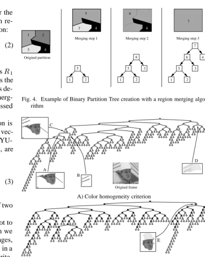
the partition of flat zones or any other pre-computed partition (for example the initial partition of 3.b), the algorithm merges neighboring regions following a homogeneity criterion until a single region is obtained. An example is shown in Fig.4. The o-riginal partition involves four regions and the algorithm merges them in three steps. In the first step, the pair of most similar regions, 1 and 2, are merged to create region 5. Then, region 5 is merged with region 3 to create region 6. Finally, region 6 is merged with region 4 and this creates region 7 corresponding to the region of support of the whole image. In this example,
the merging sequence is: (1;2)j(5;3)j(6;4). This merging
se-quence progressively defines the Binary Partition Tree as shown in Fig. 4.
Following the terminology of section II-A, it can be seen that, since the segmentation algorithm keeps on merging regions until a single region is obtained, the tree construction only makes use of the merging order and the region model whereas the merging criterion is trivial. In order to create the Binary Partition Trees used to illustrate the processing examples discussed in this pa-per, we have used a merging algorithm following the color ho-mogeneity criterion described in [7]. Let us define the merging
orderO(R
1 ;R
2
)and the region modelM
Merging order: At each step the algorithm looks for the
pair of most similar regions. The similarity between
re-gionsR
1and R
2is defined by the following expression:
O(R 1 ;R 2 )=N 1 jjM R 1 M R 1 [R 2 jj 2 (2) +N 2 jjM R2 M R1[R2 jj 2 whereN 1and N
2are the numbers of pixels of regions
R 1 andR 2and jj:jj 2denotes the L 2norm. M Rrepresents the
model for regionR. It consists of three constant values
de-scribing the YUV components. The interest of this merg-ing order, compared to other classical criteria, is discussed in [7].
Region model: As mentioned previously, each region is
modeled by a constant YUV value.M
Ris therefore a
vec-tor of 3 components. During the merging process, the
YU-V components of the union of 2 regions,R
1and R 2, are computed as follows [7]: ifN 1 <N 2 ) M R1[R2 =M R2 ifN 2 <N 1 ) M R1[R2 =M R1 ifN 1 =N 2 ) M R1[R2 =(M R1 +M R2 )=2 (3) As can be seen, ifN 1 6=N
2, the model of the union of two
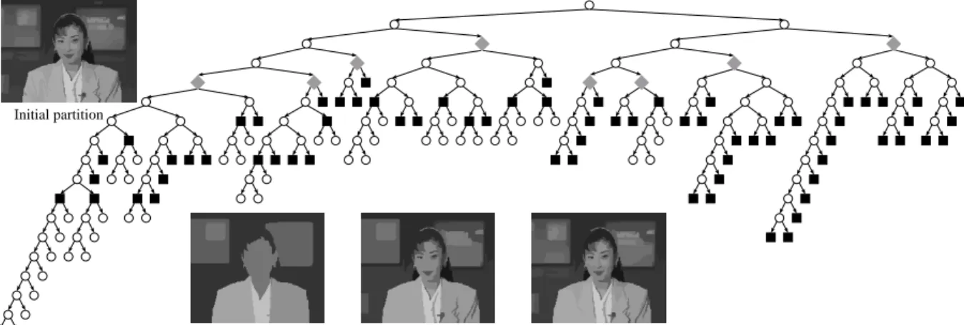
regions is equal to the model of the largest region. It should be noticed that the homogeneity criterion has not to be restricted to color. For example, if the image for which we create the Binary Partition Tree belongs to a sequence of images, motion information should also be used to generate the tree: in a first stage, regions are merged using a color homogeneity crite-rion, whereas a motion homogeneity criterion is used to merge regions in the second stage [6]. Fig. 5 shows an example of the
Foreman sequence. In Fig. 5.A, the Binary Partition Tree has
been constructed exclusively with the color homogeneity criteri-on described above. In this case, it is not possible to ccriteri-oncentrate the information about the foreground object (head and shoul-der regions of Foreman) within a single sub-tree. For example,
the face mainly appears in the sub-tree hanging from regionA,
whereas the helmet regions are located below regionD. In
prac-tice, the nodes that are close to the root have no clear meaning because they are not homogeneous in color. Fig. 5.B presents an example of Binary Partition Tree created with color and mo-tion criteria. The nodes appearing in the lower part of the tree as white circles correspond to the color criterion, whereas the dark squares correspond to a motion criterion. The motion criterion is formally the same as the color criterion except that the YUV color distance is replaced by the YUV Displaced Frame Differ-ence. As can be seen, the process starts with the color criterion as in Fig. 5.A and then, when a given Peak Signal to Noise Ra-tio (PSNR) is reached, it changes to the moRa-tion criterion. Using motion information, the face and the helmet now appear as a
single regionE.
Additional information of previous processing or detection al-gorithms can also be used to generate the tree in a more robust way. For instance, a mask of an object included in the image can be used to impose constraints on the merging algorithm in such a way that the object itself is represented with only one n-ode in the tree. Typical examples of such algorithms are face, skin, character or foreground object detection. An example is
1 2 3 4 3 4 4 5 6 1 2 1 2 3 1 2 3 4 5 5 6 7 6 5 Original partition Merging step 3 Merging step 2 Merging step 1 7
Fig. 4. Example of Binary Partition Tree creation with a region merging algo-rithm Original frame C A B D
A) Color homogeneity criterion
E B) Color and motion homogeneity criteria Fig. 5. Examples of creation of Binary Partition Tree
illustrated in Fig. 6. Assume for example that the original
Chil-dren image sequence has been analyzed so that the masks of the
two foreground objects (children) are available. If the merging algorithm is constrained to merge regions within each mask be-fore dealing with the remaining regions, the region of support of each mask will be represented as a single node in the resulting Binary Partition Tree. In Fig. 6, the nodes corresponding to the background and the two foreground objects are represented by squares. The three sub-trees further decompose each object into elementary regions.
In the sequel, we assume that the Binary Partition Tree has been created and we discuss the interest of this representation for various image processing tasks.
IV. INFORMATION RETRIEVAL
A. Detection/Recognition tools
One of the key issues of information retrieval is to be able to efficiently identify objects corresponding to a given query. In the sequel, we describe a simple example of circular objects detection but the approach can be used for any criterion that has to be optimized over a set of regions. The circularity is defined as the squared perimeter divided by the area and is minimum for
circular objects for which it is equal to4.
Bina-Original image
Background Object 1
Object 2
Fig. 6. Example of partition tree creation with restriction imposed by object masks
ry Partition Tree is a particularly attractive representation since it proposes a reduced number of regions which are assumed to be the most homogeneous for different scales. Suppose that a size descriptor and a perimeter descriptor have been assigned to each node of the tree. Now consider the example presented in
Fig. 7. In this case, the initial partition is made ofN = 100
regions. As a result, the set of regions represented by the Binary
Partition Tree equals2N 1 =199. So, the algorithm has to
measure the circularity of only 199 regions. In the tree of Fig. 7, the circular regions have been represented by dark squares. A spatial representation of these regions is also show. They cor-respond to the letters “o” appearing in “Welcome to the MPEG World” message and to various circular components of the im-age. This approach can easily be extended to deal with generic shape recognition tasks. In this case, a general shape descriptor should be assigned to each node.
Note that the tree structure introduces a notion of scalabili-ty in the description itself. Indeed, one region is described by its own descriptors but also by the set of descriptors of its chil-dren. Assume, for example, that the luminance information of a region is described by a constant value. This is a very crude
approximation. However, for a given region R, this
approxi-mation can be improved if the set of luminance descriptors of
all the regions included inR are considered. The most
accu-rate description is obtained when the descriptors of the leaves
of the sub-tree hanging fromRare considered. Finally, the tree
structure is also an attractive solution to encode the descriptors. Indeed, the tree can be used to take benefit from the correlation and inheritance relationships between descriptors.
B. Visual browsing
The previous example involves the evaluation and the opti-mization of a local criterion independently on each region. By contrast, the following browsing example discusses an approach where the optimization is global on the entire tree structure.
Browsing is an important functionality for information re-trieval. Most of the time, the user would like to have a rough idea on the query results. The goal is not to visualize a high quality image, but simply to be able to discard or not the query result. This issue is not trivial if the transmission channel be-tween the client and the server has a reduced bandwidth. A Bi-nary Partition Tree is also very attractive representation to deal with such a functionality. Indeed, as shown in [15], partition trees in general are appropriate to define optimum pruning s-trategies in the rate/distortion sense with restriction on the rate
Circular objects Original frame
Binary Partition Tree
Fig. 7. Example of detection of circular objects (initial partition with 100 re-gions).
to be transmitted or the distortion of the coded image. Let us discuss this approach.
Assume that the visual information is transmitted by select-ing some regions described by the Binary Partition Tree and by sending their contours plus a constant color value per region. The definition of the coding strategy consists in finding the best
partition created by regions,R
i, contained in the tree such that
the global distortion, D, is minimized and the rate or coding
cost,C(in bits), is lower than a given budget. Note that in this
section, we assume that the goal is to minimize the distortion under a rate constraint. It is also possible to minimize the rate under a distortion constraint. The only modification would be to
exchange the roles ofDandC.
As discussed in [15], the first step consists in analyzing the
rate C(R
i
)and distortionD(R
i
) associated to each regionR
i
in the tree. The computation of the distortion is rather straight-forward and the Squared Error between the original and coded frames can be used:
D(R i ) = P ~ p2R i (I Y ( ~p) M Y Ri ) 2 + ((I U ( ~p) M U Ri ) 2 +(I V ( ~p) M V Ri ) 2 ) (4)
where the parameter is used to balance the luminance and
the chrominance distortion. In this equation,I
Y ( ~p),I U ( ~p)and I V
( ~p) denote the luminance and chrominance components of
the pixel~pwhereasM
Y Ri ,M U Ri andM V Ri
represent the compo-nents of the region model.
The situation is more complex for the computation of the rate
C(R i
). Indeed the rate associated to a region is composed of
24 bits for the color information plus a certain number of bits for the shape information. In practice, most of the contour cod-ing techniques for partition do not process independently each region because a contour is always shared by two regions. In order to avoid the problem of optimization with complex depen-dencies between regions, we have used the following approxi-mation of the contour rate: an average number of bits necessary to encode a contour point has been estimated. This number is
denoted byBPCP(Bits Per Contour Point). We have assumed
that the contour rate assigned to a region is equal to this average
figure multiplied by the region perimeter,@R
i, divided by two
(each contour point is shared by two regions). As a result, the rate per region is given by:
C(R i
)=24+(BPCP @R i
Distortion: D; Rate: C; Budget rate: C
0; Lagrange
param-eter: ;
l
=0; /* Compute D and C for a very low */
BottomUpAnalysis(Input: l, Output: C;D); if C<C 0 then f no solution; exit;g C l =C; D l =D; h =10 20
; /* Compute D and C for a very high */
BottomUpAnalysis(Input: h, Output: C;D); if C>C 0 then f no solution; exit;g C h =C; D h =D;
do f /* Find the optimum value */
=(D l D h )=(C h C l ); BottomUpAnalysis(Input: , Output: C;D); if C<C 0 then f C h =C; D h =D; g else f C l =C; D l =D; g g until (CC 0)
Fig. 8. Algorithm for Rate-distortion optimization
The rate/distortion optimization itself relies on the technique discussed in [11], [12], [13]. The problem can be formulated
as the minimization of the distortionD =
P Ri
D(R i
)of the
image with the restriction that the total rateC =
P Ri
C(R i
)is
below a given budgetC
0. Note that both the rate and the
distor-tion have to be additive over the regions. It is well known that this problem can be reformulated as the minimization of the
La-grangian:D+Cwhereis the so-called Lagrange parameter.
Both problems have the same solution if we find
such that
Cis equal (or very close) to the budget. Therefore, the problem
consists in using the Binary Partition Tree to find a set of regions creating a partition such that:
MinD+ C, with such thatCC 0 (6)
Assume, in a first step, that the optimum
is known. The definition of the best partition can be done by a bottom-up anal-ysis of the Binary Partition Tree. To initialize the process, all the leaves of the Binary Partition Tree are assumed to belong to the optimum solution. Then, one checks if it is better to code the area represented by two sibling nodes as two independent
regionsfX
1 ;X
2
gor as a single regionX (the common parent
node ofX
1and X
2). The selection of the best choice is done by
comparing the Lagrangian ofXwith the sum of the Lagrangians
ofX 1and X 2: IfD(X)+ C(X) P i=1;2 D(X i )+ C(X i )
then, encodeXas a single region
else, encodeX
1and X
2as 2 independent regions
(7)
The best encoding strategy (encodeXas itself or as the union
of its children) is stored in X together with the corresponding
Lagrangian value. The procedure is iterated up to the root node and defines the best coding strategy.
In practice, of course, the optimum
parameter is not known and the previous bottom-up analysis of the Binary Partition Tree
is embedded in a loop that searches for the bestparameter.
The computation of the optimumparameter can be done with
a gradient search algorithm. The algorithm starts with a very
high value
h ( 10
20
) and a very low value
l (0) of
. For
each value of, the bottom-up optimization procedure described
above is performed. This results in two partitions that should
correspond to ratesC
hand C
lrespectively below and above the
budget. If none of these rates is close enough to the budget, a
new Lagrange parameter is defined as=(D
l D h )=(C h C l ).
The procedure is iterated until the rate gets close enough to the budget. The algorithm is described in pseudo-code in Fig. 8. In
practice, the optimum
parameter is found with few iterations, typically less than ten iterations. The bottom-up analysis itself is not expensive in terms of computation since the algorithm has simply to perform the comparison of equation 7 for all nodes of the tree.
Fig. 9 shows a Binary Partition Tree corresponding to a ini-tial partition involving 100 regions. If this original image would have to be transmitted for browsing, and assuming that a coding strategy involving the coding of the contours with chain code and of a constant color value for each region is used, the cost in term of bits would be equal to 14000. With respect to the original image in QCIF format, this strategy already provides a reasonable compression factor: the original image involves 176*144*24 = 608256 bits and the corresponding compression factor is equal to 43. However, for visualization purposes, this strategy is not optimum. We show in Fig. 9 three examples of coded images at 3000, 7000 and 11000 bits. As can be seen, the image coded at 11000 bits is visually equal to the initial partition image. In the case where the transmission rate is very low, high-er compression factors may be used while allowing the ushigh-er to have an idea about the image content. Two coding strategies are
Initial partition
Coding with 3000 bits Coding with 7000 bits Coding with 11000 bits
Fig. 9. Examples of pruning for visualization: Black squares (gray rhombus) in the tree define the optimum solution in the rate-distortion sense for 11000 bits (3000 bits).
shown in the tree representation of Fig. 9. The first one corre-sponds to the optimum solution for 11000 bits and is shown with dark squares. The second one shown in gray rhombus give the optimum solution at 3000 bits. As can be seen, for low bit rates, the algorithm selects regions close to the root of the tree. For higher bit rates, a large number of small regions providing de-tails about the image content can be transmitted. Finally, Fig. 10 gives the complete rate/distortion curve. One can see the evolu-tion of the visual quality as a funcevolu-tion of the number of regions introduced in the partition.
V. SEGMENTATION A. Direct approach
The Binary Partition Tree representation is particularly suit-able to generate segmentation results. Two examples of seg-mentation strategies are discussed in the following. The first one (Fig. 11) is a segmentation following a “direct” approach. It consists in merging the regions that are the most similar until a termination criterion is reached. Examples of termination crite-ria are the number of regions or the PSNR between the original and the modeled images. Note that, with respect to the segmen-tation framework described in section II-A, the creation of the Binary Partition Tree has fixed the merging order. The merging criterion (here a termination criterion) is used in a second phase without modifying the order. Therefore, this approach is similar to the one used for connected operators.
The Binary Partition Tree representation is particularly suit-able for the “direct” segmentation approach. Indeed, the merg-ing sequence, which has been used to create the tree, defines the similarity between regions. It assumes that the most simi-lar regions are merged first. Therefore, the segmentation can be computed by progressively deactivating the nodes following the merging sequence until the termination criterion is met (required number of regions or PSNR). Using the same initial partition as the one of Fig. 9, we show four examples of segmentation in Fig. 11. In all cases, the termination criterion is defined by the number of regions. 14 12 10 8 6 4 2 0 Rate in Kbits 2500 2000 1500 1000 500 0 Distortion
Fig. 10. Rate/distortion curve for the partition tree of Fig. 9
a) b)
c) d)
Fig. 11. Four examples of “direct” segmentation: a) 50 regions, b) 15 regions, c) 8 regions, d) 2 regions
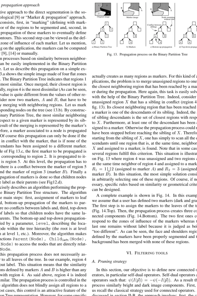
B. Marker & propagation approach
An alternative approach to the direct segmentation is the so-called morphological [9] or “Marker & propagation” approach. The strategy consists, first, in “marking” (defining with mark-ers) the interior of the regions to be segmented and, second, in performing a propagation of these markers to eventually define the regions contours. This second step can be viewed as the def-inition of the zone of influence of each marker. Let us mention, that depending on the application, the markers can be computed automatically [9], [14] or manually.
Propagation processes based on similarity between neighbor-ing regions can be easily implemented in the Binary Partition Tree structure. Let us describe this propagation on a simple ex-ample. Fig. 13.a shows the simple image made of four flat zones used in Fig. 4. The Binary Partition Tree indicates that regions 1 and 2 are the most similar. Once merged, their closest region is region 3. Finally, region 4 is the most dissimilar (As can be seen, its gray level value is quite different from the values of other
re-gions). Consider now two markers, AandB, that have to be
propagated by merging with neighboring regions. Let us mark the two corresponding nodes on the tree (see 13.b). By construc-tion of the Binary Particonstruc-tion Tree, the most similar neighboring region with respect to a given marker is represented by its sib-ling and the result of the merging is represented by the marker’s parent. Therefore, a marker associated to a node is propagated to its parent. Of course this propagation can only be done if the sibling is not in conflict with the marker, that is if none of the sibling’s descendants has been assigned to a different marker. In the example of Fig 13.c, the first marker to be propagated is
the markerAcorresponding to region 2. It is propagated to
it-s parent, that iit-s region 5. At thiit-s level, the propagation hait-s to stop because there is a conflict between the marker of region 5
(markerA) and the marker of region 3 (markerB). Finally a
top-down propagation of markers is done so that children nodes have the same label as their parents (see Fig12.d).
Fig. 12 precisely describes an algorithm performing the prop-agation on the Binary Partition Tree structure. The algorithm works in three main steps: first, assignment of markers to leaf nodes, second, bottom-up propagation of the markers to par-ents if there are no conflicts between labels and, third, top-down propagation of labels so that children nodes have the same la-bel as their parents. The bottom-up and top-down
propagation-s are controlled by a parameter, level, describing the
loca-tion of the node within the tree hierarchy (the root is at level 0, its children at level 1, etc.). Moreover, the algorithm makes
use of the functionsParent(Node), Childleft(Node),
Childrigth(Node)to access the nodes that are directly
relat-ed to a givenNode.
Note that this propagation process does not necessarily as-sign a marker to all leaves of the tree. In our example, region 4 remains without label. This situation means that the similarity
between regions defined by markersAandBis higher than any
combination with region 4. As said above, region 4 is indeed the most dissimilar. The propagation process is controlled in the sense that the algorithm does not blindly assign all regions to a marker. In most cases, this control is an attractive feature of the Binary Partition Tree representation. However, for some specific applications, one would like to use a propagation algorithm that
1 2 3 4 0000 0000 0000 1111 1111 1111 0000 0000 0000 0000 1111 1111 1111 1111 00000000 0000 1111 1111 1111 0000 0000 0000 0000 1111 1111 1111 1111 000 000 000 111 111 111 Original image A B A B Marker image
a) Binary Partition Tree b) Markers
A A B A B siblings Conflict between c) Bottom-up propagation Node remaining without label A B A A d) Top-down propagation 1 2 3 4 5 6 7
Fig. 13. Propagation process on the Binary Partition Tree
actually creates as many regions as markers. For this kind of ap-plications, the problem is to merge unassigned regions to one of the closest neighboring region that has been reached by a mark-er during the propagation. Hmark-ere again, this task is easily solved with the help of the Binary Partition Tree. Indeed, consider an
unassigned regionX that has a sibling in conflict (region 4 in
fig. 13). Its closest neighboring region that has been reached by a marker is one of the descendants of its sibling. Indeed, the set of sibling descendants is the set of closest regions with respect
toX. Furthermore, at least one of the descendant has been
as-signed to a marker. Otherwise the propagation process could not
have been stopped before reaching the sibling ofX. Therefore,
starting from the sibling ofX, one has simply to scan all the
de-scendants until one region that is, at the same time, neighbor of
X and assigned to a marker, is found. Note that in some cases,
several regions fulfill this criterion. This situation is illustrated on Fig. 13 where region 4 was unassigned and two regions are at the same time neighbor of region 4 and assigned to a marker:
R 1
= 1 S
2(assigned to markerA) and R
2
= 3(assigned to
markerB). In this situation, the most simple solution consists
in arbitrarily selecting one of these regions. Of course, if nec-essary, specific rules based on similarity or geometrical criteria can be designed.
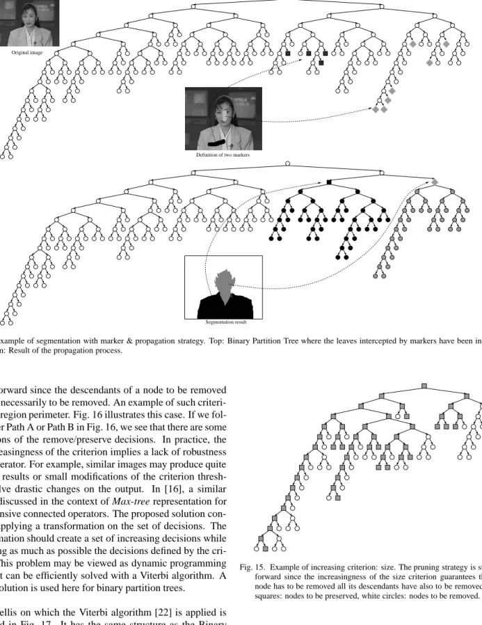
A complete example is shown in Fig. 14. In this example, we assume that a user has defined two markers (dark and gray). The first step is to assign the markers to the leaves of the tree (Fig. 14.Top). Then, the propagation process creates three con-nected components (Fig. 14.Bottom). The two first ones cor-respond to the zones of influence of the markers whereas the last one remains without label because it is judged as being “too different”. As can be seen, the face and shoulders regions defined by the markers have been properly segmented and the background has been merged with none of these regions.
VI. FILTERING TOOLS
A. Pruning strategy
In this section, our objective is to define new connected op-erators, in particular self-dual operators. Self-dual operators are
operators such that: (I( ~p)) = ( I( ~p)). As a result they
process similarly bright and dark image components. First, let us recall the classical strategy used for connected operators. As discussed in section II-B, the approach involves: first, the cre-ation of a tree representcre-ation of the image (Max-tree or
Min-N
l: Set of nodes at level l;
Node->label: label of marker;
Node->conflict: States if the two sub-trees of node correspond to differ-ent markers;
/* Initialization */ for all nodes in the tree: f Node->label = void; Node->conflict = void;g
Assign a label to leaves that overlap with a marker;
/* Bottom-up propagation of markers */ for (level = level max; level 0; level--)f
for all nodes Node 2N
level that are non-leaf nodes
f
/* Analyze the conflicts */ if ( (Childleft(Node)->label != void) && (Childright(Node)->label !=
void) &&
(Childleft(Node)->label != (Childright(Node)->label))
Node->conflict = CONFLICT
if ( (Childleft(Node)->conflict == CONFLICT) ||
(Childright(Node)->conflict == CONFLICT))
Node->conflict = CONFLICT
/* If there is no conflict, propagate the label from children */ if (Node->conflict == void)f
if (Childleft(Node)->label != void)
Node->label = Childleft(Node)->label;
else if (Childright(Node)->label != void)
Node->label = Childright(Node)->label;
g
gg
/* Propagate label from parent to children (in absence of conflicts) */ for (level = 1; level level max; level++)f
for all nodes Node 2N level
f
if ((Parent(Node)->conflict != CONFLICT) && (Node->conflict != CONFLICT)) Node->label = Parent(Node)->label;
gg
Fig. 12. Algorithm for marker propagation in the Binary Partition Tree structure
tree1), second, the assessment of a criterion for each node of the
tree and third, the definition of a tree pruning strategy. The prun-ing defines a new partition and each region is represented by a constant value (minimum in the case of Max-tree and maximum in the case of Min-tree).
Mathematically, a criterionCassessed on a regionRis said
to be increasing if the following property holds:
8R 1 R 2 )C(R 1 )C(R 2 ) (8) 1
the Min-tree can be defined as the Max-tree of the opposite of the original image.
Assume that all nodes corresponding to regions where the cri-terion value is lower than a given threshold should be removed by merging. If the criterion is increasing, the pruning strategy is straightforward: merge all nodes that should be removed. It is indeed a pruning strategy since the increasingness of the criteri-on guarantees that if a node has to be removed all its descendants have also to be removed. An example of Binary Partition Tree with increasing decision criterion is shown in Fig. 15. The cri-terion used to create this example is the size, measured as the number of pixels belonging to the region.
Original image
Definition of two markers
Segmentation result
Fig. 14. Example of segmentation with marker & propagation strategy. Top: Binary Partition Tree where the leaves intercepted by markers have been indicated. Bottom: Result of the propagation process.
straightforward since the descendants of a node to be removed have not necessarily to be removed. An example of such criteri-on is the regicriteri-on perimeter. Fig. 16 illustrates this case. If we fol-low either Path A or Path B in Fig. 16, we see that there are some oscillations of the remove/preserve decisions. In practice, the non-increasingness of the criterion implies a lack of robustness of the operator. For example, similar images may produce quite different results or small modifications of the criterion thresh-old involve drastic changes on the output. In [16], a similar issue is discussed in the context of Max-tree representation for anti-extensive connected operators. The proposed solution con-sists in applying a transformation on the set of decisions. The transformation should create a set of increasing decisions while preserving as much as possible the decisions defined by the cri-terion. This problem may be viewed as dynamic programming issue that can be efficiently solved with a Viterbi algorithm. A similar solution is used here for binary partition trees.
The trellis on which the Viterbi algorithm [22] is applied is illustrated in Fig. 17. It has the same structure as the Binary
Partition Tree except that each nodeN
kof the Binary Partition
Tree corresponds to two trellis states: preserveN
P k and remove N R k
. The two states of each child node are connected to the two states of its parent. However, in order to avoid non-increasing decisions, the preserve state of a child is not connected to the
remove state of its parent. As a result, the trellis structure
guar-antees that if a node has to be removed its children have also to
Fig. 15. Example of increasing criterion: size. The pruning strategy is straight-forward since the increasingness of the size criterion guarantees that if a node has to be removed all its descendants have also to be removed. Gray squares: nodes to be preserved, white circles: nodes to be removed.
be removed. The cost associated to each state is used to compute the number of modifications the algorithm has to do to create an increasing set of decisions. If the criterion value states that the node of the Binary Partition Tree has to be removed, the cost associated to the remove state is equal to zero (no modification) and the cost associated to the preserve state is equal to one (one modification). Similarly, if the criterion value states that the
n-Path A
Path B
Fig. 16. Example of non-increasing criterion: perimeter. The pruning strategy is not straightforward since the criterion does not guarantee that if a node has to be removed all its descendants have also to be removed (see decisions along path A or path B). Gray squares: nodes to be preserved, white circles: nodes to be removed.
ode has to be preserved, the cost of the remove state is equal
to one and the cost of the preserve state is equal to zero2. The
cost values appearing in Fig. 17 assume that nodesN
1, N
4and N
5should be preserved and that
N 2and
N
3should be removed.
The goal of the Viterbi algorithm is to define the set of decisions such that: Min X k Cost(N k
)such that the decisions are increasing (9)
To find the optimum set of decisions, a set of paths going from all leaf nodes to the root node is created. For each node, the path can go through either the preserve or the remove state of the trel-lis. The Viterbi algorithm is used to find the paths that minimize the global cost at the root node. Note that the trellis structure itself guarantees that this optimum decision is increasing. The optimization is achieved in a bottom-up iterative fashion. For each node, it is possible to define the optimum paths ending at the preserve state and at the remove state.
Let us consider a nodeN
k and its preserve state
N P k
. A
pathPath
k is a continuous set of transitions between
n-odes(N
!N
)defined in the trellis:
Path k =(N !N )[(N !N )[:::[(N !N ! ).
The pathPath
P k
starting from a leaf node and ending at that state is composed of two sub-paths: the first one,
Path P;Left k
, comes from the left child and the second one,
Path P;Right k
, from the right child (see Fig. 18). In both cases, the path can emerge either from the preserve or from
the remove state of the child nodes. IfN
k1 and N
k2 are
respectively the left and the right child nodes ofN
k, we 2
Although some modifications may be much more severe than others, the cost choice has no strong effect on the final result. This issue of cost selection is similar to the hard versus soft decision of the Viterbi algorithm in the context of digital communications [22]. N2 N3 N1 N4 N5 N1,remove N1,preserve N3,remove cost:1 cost:0 N4,preserve N5,preserve N4,remove cost:0 cost:1 cost:0 cost:1 N2,preserve N3,preserve N2,remove cost:1 cost:0 cost:1 cost:0 N5,remove Binary Partition Tree
Trellis for the Viterbi algorithm
Fig. 17. Creation of the trellis structure for the Viterbi algorithm. A circular (square) node on the Binary Partition Tree indicates that the criterion value states that the node has to be removed (preserved). The trellis on which the Viterbi algorithm is run duplicates the structure of the Binary Partition Tree and defines a preserve state and a remove state for each node of the tree. Paths from remove states to child preserve states are forbidden so that the decisions are increasing.
have: Path P;Left k = Path R k 1 S (N R k 1 !N P k ) or Path P k 1 S (N P k 1 !N P k ) Path P;Right k = Path R k2 S (N R k2 !N P k ) or Path P k 2 S (N P k 2 !N P k ) Path P k = Path P;Left k S Path P;Right k (10)
The cost of a path is equal to the sum of the costs of its individual state transitions. Therefore, the optimum path (path of lower cost) for each child can be easily selected.
IfCost(Path R k 1 ) < Cost(Path P k 1 ) thenfPath P;Left k = Path R k1 S (N R k1 !N P k ); Cost(Path P;Left k ) = Cost(Path R k1 );g elsefPath P;Left k = Path P k1 S (N P k1 !N P k ); Cost(Path P;Left k ) = Cost(Path P k1 );g 5mm]IfCost(Path R k2 ) < Cost(Path P k2 ) thenfPath P;Right k = Path R k2 S (N R k2 !N P k ); Cost(Path P;Right k ) = Cost(Path R k2 );g elsefPath P;Right k = Path P k2 S (N P k2 !N P k ); Cost(Path P;Right k ) = Cost(Path P k 2 );g Cost(Path P k ) = Cost(Path P;Left k ) + Cost(Path P;Right k ) + Cost(N P k ); (11)
In the case of the remove state,N
R k
, the two sub-paths can only come from the remove states of the children. So, no selection has to be done. The path and its cost are
con-structed as follows: Path R;Left k = Path R k 1 S (N R k 1 !N R k ); Path R;Right k = Path R k 2 S (N R k 2 !N R k ); Path R k = Path R;Left k S Path R;Right k ; Cost(Path R k ) = Cost(Path R k 1 )+Cost(Path R k 2 ) + Cost(N R k ); (12)
This procedure is iterated in a bottom-up fashion until the root node is reached. One path of minimum cost ends at the preserve state of the root node and another path ends at the remove state of the root node. Among these two paths, the one of minimum cost is selected. This path connects the root node to all leaves and the states it goes through define the final decisions. By construction, these decisions are increasing and they are as close as possible to the original decisions.
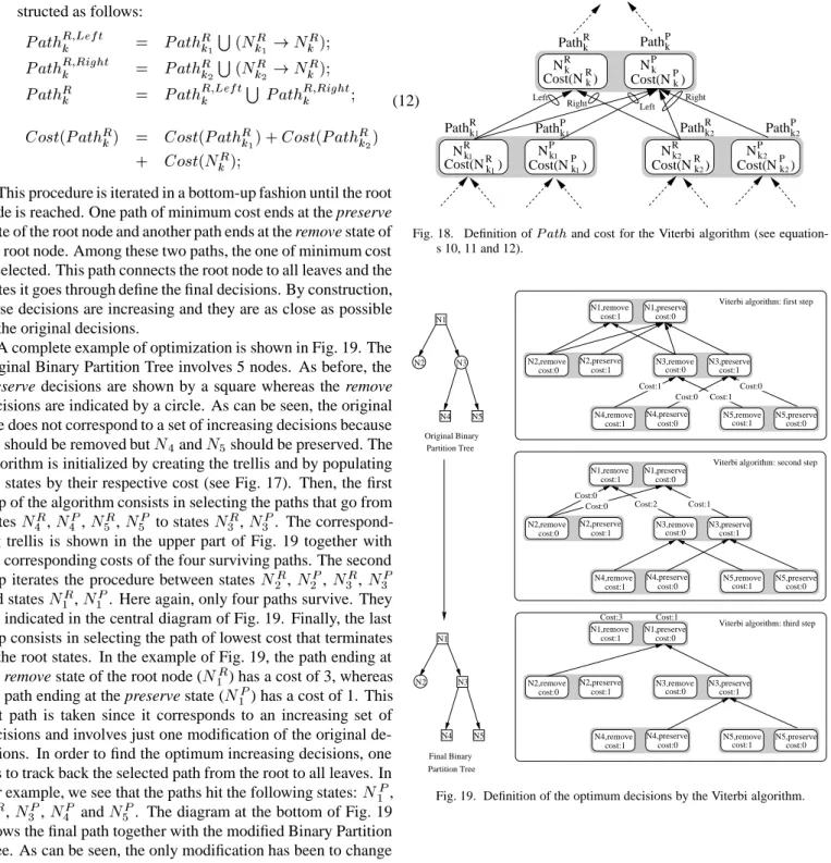
A complete example of optimization is shown in Fig. 19. The original Binary Partition Tree involves 5 nodes. As before, the
preserve decisions are shown by a square whereas the remove
decisions are indicated by a circle. As can be seen, the original tree does not correspond to a set of increasing decisions because
N
3should be removed but
N 4and
N
5should be preserved. The
algorithm is initialized by creating the trellis and by populating the states by their respective cost (see Fig. 17). Then, the first step of the algorithm consists in selecting the paths that go from
statesN R 4, N P 4, N R 5, N P 5 to states N R 3, N P 3 . The
correspond-ing trellis is shown in the upper part of Fig. 19 together with the corresponding costs of the four surviving paths. The second
step iterates the procedure between statesN
R 2 , N P 2 ,N R 3 ,N P 3 and statesN R 1 ,N P 1
. Here again, only four paths survive. They are indicated in the central diagram of Fig. 19. Finally, the last step consists in selecting the path of lowest cost that terminates at the root states. In the example of Fig. 19, the path ending at
the remove state of the root node (N
R 1
) has a cost of 3, whereas
the path ending at the preserve state (N
P 1
) has a cost of 1. This last path is taken since it corresponds to an increasing set of decisions and involves just one modification of the original de-cisions. In order to find the optimum increasing decisions, one has to track back the selected path from the root to all leaves. In
our example, we see that the paths hit the following states:N
P 1 , N R 2 , N P 3 , N P 4 and N P
5. The diagram at the bottom of Fig. 19
shows the final path together with the modified Binary Partition Tree. As can be seen, the only modification has been to change
the decision of nodeN
3and the resulting set of decisions is
in-creasing.
A complete example of decisions modification is shown in Fig. 20. The original Binary Partition Tree corresponds to the one shown in Fig. 16. The Viterbi algorithm has to modify 5 de-cisions along path A and one decision along path B (see Fig. 16) to get the optimum set of increasing decisions.
To summarize this section, let us say that the pruning strat-egy can be applied directly on the tree if the decision criterion is increasing (size is a typical example). In the case of a non-increasing criterion such as the perimeter, the Viterbi algorithm can be used to modify the smallest number of decisions so that increasingness is obtained. These modifications define a prun-ing strategy. R k Cost(N ) NRk NPk Cost(N )Pk NPk Cost(N )Pk NRk Cost(N )Rk Nk Cost(N )Pk P NRk R k Cost(N )1 1 1 1 2 2 2 2 PathkR PathkP PathkR2 PathkP1 PathkP2 PathkR1 Left Right Left Right
Fig. 18. Definition ofPathand cost for the Viterbi algorithm (see
equation-s 10, 11 and 12). N2 N3 N1 N4 N5 N1,remove N1,preserve N3,remove cost:1 cost:0 N4,preserve N5,preserve N4,remove cost:0 cost:1 cost:0 cost:1 N2,preserve N3,preserve N2,remove cost:1 cost:0 cost:1 cost:0 N5,remove Cost:0
Cost:0 Cost:2 Cost:1 N1,remove N1,preserve N3,remove cost:1 cost:0 N4,preserve N5,preserve N4,remove cost:0 cost:1 cost:0 cost:1 N2,preserve N3,preserve N2,remove cost:1 cost:0 cost:1 cost:0 N5,remove Cost:1 Cost:0 Cost:1 Cost:0 N1,remove N1,preserve N3,remove cost:1 cost:0 N4,preserve N5,preserve N4,remove cost:0 cost:1 cost:0 cost:1 N2,preserve N3,preserve N2,remove cost:1 cost:0 cost:1 cost:0 N5,remove N2 N3 N1 N4 N5 Original Binary Partition Tree Partition Tree Final Binary Cost:3 Cost:1
Viterbi algorithm: first step
Viterbi algorithm: third step Viterbi algorithm: second step
Fig. 19. Definition of the optimum decisions by the Viterbi algorithm.
B. Filtering example
Once the tree has been pruned, the output partition is comput-ed and each region is modelcomput-ed by a constant value. In the case of anti-extensive connected operators, the minimum gray level value of the pixels in the original image is used. Here, since we are interested in self-dual operators, a self-dual model has to be used. Examples of self-dual models are the mean or the median of the original pixel values. In the following we assume that the median is used.
A first example of size-oriented simplification is shown in Fig. 21.a. The size threshold has been set to 50 pixels. This result may be surprising because a large number of regions s-maller than 50 pixels are still visible in the filtered image (the
Fig. 20. Set of increasing decisions resulting from from the use of the Viterbi algorithm on the original tree of Fig. 16. Five decisions along path A and one decision along path B have been modified. Gray squares: nodes to be preserved, white circles: nodes to be removed.
texture of the fish for example). To understand this result, let us analyze the example of Binary Partition Tree shown in the left side of Fig. 22 (Note that this tree is presented here as a simple illustration. It is not the tree used to generate the example of Fig. 21). In this tree, one can see a large number of configura-tions where one node has to be removed whereas its sibling has to be preserved. Note that since the criterion is increasing, the parent of these two nodes has to be preserved. In terms of re-gions, this configuration means that one of the siblings as well as the parent correspond to large regions whereas the other sibling is of small size. Fig. 23 illustrates this issue on a very simple
example: RegionsR
1and R
2should be preserved because they
are of large size, whereas regionR
3 =R
1 nR
2is of small size.
It should be removed but in the final partition, the space
corre-sponding toR
1 nR
2 will appear as a connected component of
small area.
In section II-B, we have illustrated the example of an area opening and we have seen that the filtered image involves a large number of small regions (potentially all regions that are not maxima). In fact, once a regional maxima has reached (by merging) the size threshold, it is not merged anymore with its neighboring regions even if these neighboring regions are smal-l. In the example of Fig. 22.left, we have the same issue: once a node corresponds to a region larger than 50 pixels, it is not merged with its sibling even if the sibling is small.
For certain applications, it may be necessary to force the oper-ator to produce an output image where all flat zones are guaran-teed to fulfill the simplification criterion. This modification can easily be implemented using the propagation process explained in section V-B. The idea is explained in Fig. 22. The first step consists in defining the markers. These markers are all Preserve leaves as well as Preserve nodes that have two Remove children. In the example of Fig. 22, there are five markers. The second step defines the filtered partition by propagating these marker-s amarker-s in the camarker-se of the marker-segmentation demarker-scribed in marker-section V-B. Fig. 22.right shows the result of this propagation on the Binary Partition Tree. A size-oriented simplification of the Bream im-age using this strategy is presented in Fig. 21.b. All regions of
size smaller than 50 pixels have been removed.
a) b)
Fig. 21. Example of size-oriented simplification (Size threshold 50 pixels). a) simple size simplification. b) size simplification with propagation strategy
Size markers
Zones of influence of the markers
Fig. 22. Size-oriented simplification. Left) Binary Partition Tree with size criterion. The black squares indicate the size markers. Right) Definition of the zones of influence of the size markers.
R2 R3 R1 Regions of large size R2 Region of small size R3 = R1 \ R2 R1 R1 \ R2
Fig. 23. Illustration of decisions where a node has to be preserved whereas it s sibling has to be removed.
Finally, Fig. 24 illustrates two simplification criteria.
Fig. 24.b corresponds to a size criterion whereas Fig. 24.c cor-responds to a perimeter criterion. In both cases, the regions that do not fulfill the criterion have been removed by propagation of the markers as explained above. Moreover, the Viterbi algorith-m has been used in the case of the perialgorith-meter since this criterion is not increasing. The difference between the two simplification criteria can be seen in the simplification of the text appearing in the upper left corner. These filtering tools are self-dual connect-ed operators and generalize the results reportconnect-ed in [16]. They possess the attractive feature of simplifying the image while p-reserving the contour information.
VII. CODINGBINARYPARTITIONTREES
As shown in the previous sections, a Binary Partition Tree is an interesting representation to implement a large set of pro-cessing tools and functionalities. Moreover, the implementation of these processing tools can be done very efficiently since the number of image components to process is reduced to the num-ber of tree nodes which in practice ranges between a few tenth to a few thousands. Note that the time consuming part of the process is not the tree processing but the definition of the merg-ing sequence. Dependmerg-ing on the application, this comment leads
a) b)
c)
Fig. 24. Example of self-dual connected operators. a) original image. b) size-oriented simplification. c) perimeter-size-oriented simplification
to the idea of computing the tree once and of storing the repre-sentation. In this context, an important question is to know how many bits are necessary to code the full representation, that is the initial partition, the merging sequence and, for example, a color value for each region of the initial partition.
In the following, we have assumed that the partition is rep-resented in QCIF format (for information retrieval applications, the original image may be in a different format) and that the con-tours of the initial partition have been coded by a simple chain code. Table II defines the number of bits for various levels of granularity of the initial partition. As can be seen, the overall number of bits remains moderate and most of the coding cost is devoted to the initial partition. Note that the coding of the ini-tial partition has been performed with a very simple and lossless technique (chain code). If higher compression is required, more sophisticated lossy techniques could be used.
VIII. CONCLUSIONS
In this paper, we have discussed the interest of Binary Par-tition Tree representations for several image processing tasks. This representation combines a large number of regions that can be extracted from an image. Although the tree construction was not the main focus of this paper, the use of segmentation algo-rithms relying on merging techniques has been discussed. Note that this is not the only possibility and top-down or supervised approaches should be investigated. The regions contained in the tree are organized in a hierarchical structure. This organization allows the implementation of fast and sophisticated techniques (for example the marker propagation of section V-B or the Viter-bi algorithm described in section VI-A).
The processing of the Binary Partition Tree generally consist-s in defining which nodeconsist-s (and correconsist-sponding regionconsist-s) are of interest for a particular image processing task. In this frame-work, we have discussed examples of minimization of local criteria (circular object detection, section IV-A) as well as the minimization of global criteria (rate/distortion optimization for browsing functionality, section IV-B). The Binary Partition Tree gives access to some (not all) neighborhood as well as similarity relationships between regions. This feature allows the
imple-Image Number of regions of the initial partition
50 100 200
Bream 8008 bits 12376 bits 19016 bits
(78,14,8%) (73,18,9%) (66,24,10%)
Akiyo 7880 bits 12512 bits 19032 bits
(77,15,8%) (73,18,9%) (65,25,10%)
TABLE II
NUMBER OF BITS TO CODE THEBINARYPARTITIONTREE
REPRESENTATION. PERCENTAGES(n1%;n2%;n3%)INDICATE THE
BITSTREAM COMPOSITION:n1INITIAL PARTITION,n2MERGING
SEQUENCE ANDn
3COLOR VALUES. NUMBER OF BITS OF THE ORIGINAL
(UNCOMPRESSED)IMAGES INQCIFFORMAT: 608256BITS
mentation of propagation techniques that are particularly useful for segmentation applications (section V-B). Finally, pruning s-trategies lead to the definition of new connected operators. In this case, we have seen that the increasingness of the merging criterion is an important issue. In the case of a non-increasing merging criterion, a Viterbi algorithm can be used to define the pruning strategy (section VI-A). Note that the specific criteria (circularity, size, perimeter, etc) used in this paper are just sim-ple examsim-ples that were selected to explain the main issues in-volved in the representation. For a particular application, more useful and possibly more complex criteria may be used. Let us mention for instance complex shape characteristics, texture fea-tures, motion information in the case of sequences, etc. We will investigate such criteria in the future.
REFERENCES
[1] E. Breen and R. Jones. An attribute-based approach to mathematical mor-phology. In P. Maragos, R.W. Schafer, and M.A. Butt, editors, Internation-al Symposium on MathematicInternation-al Morphology, pages 41–48, Atlanta (GA), USA, May 1996. Kluwer Academic Publishers.
[2] C.R. Brice and C.L. Fenema. Scene analysis using regions. Artificial intelligence, 1:205–226, 1970.
[3] J. Crespo. Morphological Connected Filters and Intra-region Smooth-ing for Image Segmentation. PhD thesis, Georgia Institute of Technology, 1993.
[4] J. Crespo. Space connectivity and translation-invariance. In P. Maragos, R.W. Schafer, and M.A. Butt, editors, International Symposium on Math-ematical Morphology, pages 118–126, Atlanta (GA), USA, May 1996. Kluwer Academic Publishers.
[5] J. Crespo, J. Serra, and R.W. Schafer. Theoretical aspects of morphological filters by reconstruction. Signal Processing, 47(2):201–225, 1995. [6] L. Garrido and P. Salembier. Region based analysis of video sequences
with a general merging algorithm. In IX European Signal Processing Con-ference, EUSIPCO’98, volume III, pages 1693–1696, Rhodes, Greece, September, 8-11 1998.
[7] L. Garrido, P. Salembier, and D. Garcia. Extensive operators in parti-tion lattices for image sequence analysis. EURASIP Signal Processing, 66(2):157–180, April 1998.
[8] H. Heijmans. Connected morphological operators and filters for binary images. In IEEE Int. Conference on Image Processing, ICIP’97, volume 2, pages 211–214, Santa Barbara (CA), USA, October 1997.
[9] F. Meyer and S. Beucher. Morphological segmentation. Journal of Visual Communication and Image Representation, 1(1):21–46, September 1990. [10] O. Morris, M. Lee, and A. Constantinidies. Graph theory for image analy-sis: an approach based on the shortest spanning tree. IEE Proceedings, F, 133(2):146–152, April 1986.
[11] A. Ortega, K. Ramchandran, and M. Vetterli. Optimal buffer-constrained source quantization and fast approximations. In Proc. IEEE Int. Symp. Circuits and Systems, volume 1, May 1992.
rate-distorsion sense. IEEE Transactions on Image Processing, 2(2):160–175, April 1993.
[13] E. Reusens. Joint optimization of representation model and frame seg-mentation for generic video compression. EURASIP Signal Processing, 46(11):105–117, September 1995.
[14] P. Salembier. Morphological multiscale segmentation for image coding. EURASIP Signal Processing, 38(3):359–386, September 1994.
[15] P. Salembier, F. Marqu´es, M. Pard`as, R. Morros, I. Corset, S. Jeannin, L. Bouchard, F. Meyer, and B. Marcotegui. Segmentation-based video coding system allowing the manipulation of objects. IEEE Trans. on Cir-cuits and Systems for Video Technology, 7(1):60–74, February 1997. [16] P. Salembier, A. Oliveras, and L. Garrido. Anti-extensive connected
op-erators for image and sequence processing. IEEE Transactions on Image Processing, 7(4):555–570, April 1998.
[17] P. Salembier and J. Serra. Flat zones filtering, connected operators and filters by reconstruction. IEEE Transactions on Image Processing, 3(8):1153–1160, August 1995.
[18] P. Salembier, L. Torres, F. Meyer, and C. Gu. Region-based video coding using mathematical morphology. Proceedings of IEEE (Invited paper), 83(6):843–857, June 1995.
[19] J. Serra and P. Salembier. Connected operators and pyramids. In SPIE, editor, Image Algebra and Mathematical Morphology, volume 2030, pages 65–76, San Diego (CA), USA, July 1993.
[20] L. Vincent. Grayscale area openings and closings, their efficient imple-mentation and applications. In J. Serra and P. Salembier, editors, First Workshop on Mathematical Morphology and its Applications to Signal Processing, pages 22–27, Barcelona, Spain, May 1993. UPC.
[21] L. Vincent. Morphological gray scale reconstruction in image analysis: Applications and efficients algorithms. IEEE, Transactions on Image Pro-cessing, 2(2):176–201, April 1993.
[22] A.J. Viterbi and J.K. Omura. Principles of Digital Communications and Coding. Mc Graw-Hill, New York, 1979.