Strategies for wireless network control with applications to LTE

(1)

Strategies for Wireless Network

Control with Applications to LTE

Von der Fakultät für Elektrotechnik und Informationstechnik der Rheinisch-Westfälischen Technischen Hochschule Aachen

zur Erlangung des akademischen Grades eines Doktors der Ingenieurwissenschaften genehmigte Dissertation

vorgelegt von

Master of Science Xiang Xu

aus China

Berichter: Universit¨atsprofessor Dr. rer. nat. Rudolf Mathar Universit¨atsprofessor Dr.-Ing. Gerd Ascheid

Tag der m¨udlichen Pr¨ung: 15. December 2014

Diese Dissertation ist auf den Internetseiten der Universit¨atsbibliothek online verf¨ugbar.

(2)

(3)

Preface

This thesis was prepared during my time in the DFG Graduate School “Software for Mobile Communication Systems” and at the Institute for Theoretical Information Technology of RWTH Aachen University.

My deep gratitude goes to my supervisor Univ.-Prof. Dr. rer. nat. Rudolf Mathar for the encouragement and support of my work. I am also grateful for the freedom to pursue my own research interests.

Many thanks to Univ.-Prof. Dr.-Ing. Gerd Ascheid for accepting to act as the second referee for this thesis.

I would like to thank Dipl.-Ing. Henning Maier, M.Sc. Omid Taghizadeh and Dipl.-Ing. Florian Schr¨oder for critical reading of this thesis.

I would also like to thank the whole staff of the Institute for Theoretical Information Technology of RWTH Aachen University for providing a pleasant working atmosphere and exchanging interesting ideas.

Finally, I thank my family for being supportive for the last six years.

(4)

(5)

1 Introduction

With the mass deployment of long-term evolution (LTE) systems, the wireless cellu-lar network has evolved to the 4th generation (4G). The 4G mobile standards aim at providing ubiquitous connectivity and high data rate services. To avoid coverage holes, sophisticated algorithms for antenna tilting, handover and load balancing are implemented. To serve densely located indoor users, small cell technologies are de-veloped. To increase spectrum efficiency, radio resource management is performed. To minimize manual effort in adjusting network performance, self-organizing network (SON) schemes are proposed. All these functionalities make the design of network controlling strategies more challenging than ever. In order to tackle various problems during deployment and operation by numerical analysis, the cellular network has to be modeled properly.

Due to the limitation of the computational power and memory, modeling a cellular network from head to toe is extremely difficult, if possible at all. Therefore, the modeling methodology is usually divided into two levels, namely, link level modeling and network level modeling. Link level modeling concentrates on characterizing com-munication channels between transmitter-receiver pairs, while network level modeling focuses on describing communication networks on a larger scale.

In this dissertation, strategies on both link and network level for wireless network control are investigated, with emphasising on the application to LTE systems. To ac-complish this task, link level modeling of wireless channels is presented first. Based on the link level models, channel state information (CSI) feedback strategies are studied. As a feature of SON, future trends of wireless network control depend heavily on the real time status of the network. A majority of status data comes from user reports. However, due to the inevitable delay of wireless transmission, the feedback informa-tion will be outdated. Therefore, proper strategies for compensating the feedback delay are proposed in this dissertation. Furthermore, with the feedback information, self-organizing network control strategies can be deployed. Self-self-organizing network control strategies cover many different areas including handover optimization, load balancing, neighbor list optimization, etc. In this thesis, a case study is given, where transmit power management is discussed.

A unique point of this dissertation is its matching to the industrial standards made by the 3rd generation partnership project (3GPP). As a standardization body, 3GPP is a collaboration of several telecommunication associations. At the end of last century, Nortel Networks and AT&T Wireless established 3GPP as a strategic initiative to de-fine the 3G standard. Later, this initiative was turned into a larger alliance with many major vendors and operators. Now 3GPP already has six organizational partnerships

(10)

across the continents of America, Europe and Asia. Their work is extending from 3G universal mobile telecommunications system (UMTS) to 4G LTE and long-term evolution advanced (LTE-A) and possibly future 5G standards.

3GPP standards are structured as releases. Each release consists of hundreds of indi-vidual standard documents and each document may have many revised versions. LTE is firstly specified in Release 8, which by the time of finishing this thesis has already been frozen, such that no further changes will be applied to this release.

By following the 3GPP technical specifications, many realistic constraints in imple-menting wireless communication systems are considered in this work. Moreover, re-alistic constraints prevent from getting close to the theoretical optimum. Thus, this dissertation puts more focus on low complexity heuristics, which are relatively easy to implement in real systems.

Due to the author’s expertise, this thesis mainly targets at the physical layer related aspects of cellular networks, except for a small part in Chapter 4. The remainder of this dissertation is organized as follows:

In Chapter 2, preparatory information about wireless communications on both link level and network level is given. Basics about some of the key technologies of LTE are explained in this chapter.

For investigating a mobile cellular system, proper modeling of the wireless channel be-tween base stations (BSs) and mobile stations (MSs) is usually the first step. There-fore, the methodology of channel modeling is addressed in Chapter 3, particularly considering multi-antenna transmission. In LTE, to achieve high capacity, up to 4×4 multi-input multi-output (MIMO) systems are supported [8]. And later in LTE-A, it is increased to 8×8 [7]. In this work, different existing MIMO channel models, including analytical models and stochastic models, are explained in detail.

Chapter 4 tackles the problem of imperfect feedback of CSI. The feedback mecha-nism following the 3GPP LTE standards is first introduced, where the CSI must be compressed to quantized data with a few levels only. Statistical properties of the time varying wireless channel in a multi-cell network are then carefully examined. Using the statistics, novel temporal variation compensation schemes are derived and compared with the conventional ones by numerical simulations. Moreover, the hybrid automatic repeat request (HARQ), which operates in the physical layer but is controlled by the media access control (MAC) layer, is explained in this chapter. HARQ is a retrans-mission mechanism to offer better error protection. This study also shows the effects of HARQ on feedback strategies.

The main goal of cellular network control is to optimize the network performance in terms of key performance indicators (KPIs). The most popular KPIs are capacity and coverage, where capacity indicates the overall throughput in the network and coverage shows the quality of service (QoS) of the users with poor signal reception. In Chapter 5, a case study on heuristic network control strategies is given. In this case study, transmit power management in a heterogeneous network with overlayed macro-and femtocells is investigated. The optimization procedure is based on the user report,

(11)

namely, the feedback information discussed in Chapter 4. System level simulators are built to serve the purpose of testing and evaluating the algorithms.

Finally, in Chapter 6, conclusions are given. And last but not least, the evolution of wireless communication does not stop at the 4th generation. Many efforts are made to improve the technology of wireless communications, which is shaping the society and people’s daily life in a unprecedented manner. Therefore, some outlooks on potential advances of wireless technology are presented in this chapter.

Parts of this thesis and related topics have already been published in [19] [29] [43] [64] [93] [94] [95] [96] [97] [98] [99] [100] [101] [102]. A number of further publications based on this work is in preparation.

(12)

(13)

2 Preliminaries

In this chapter, some important facts of wireless networks are introduced. Firstly, the basic mathematical representation of a wireless communication link is described in Section 2.1. Secondly, the transmission technology of orthogonal frequency division multiplexing (OFDM) is presented in Section 2.2. Furthermore, multiple antenna techniques are explained in Section 2.3. Finally, the wireless cellular network is briefly discussed in Section 2.4.

2.1 Wireless communication links

A simple communication link consists of three parts, namely, transmitter, receiver and communication channel in between. The most fundamental question in wireless communications is how to recover the transmitted signals at the receiver side, or in another word, to remove the distortion caused by the communication channel.

In wireless communication systems, while the transmitter and receiver can be designed and controlled, the wireless channel can not be manipulated. Thus, in scientific works, accurate channel models are desired, in order to recreate a close-to-reality environment for testing ideas and developing new concepts.

In a single antenna system, the baseband received signal after multi-path propagation can be written as:

y(t) = τmax

Z

0

h(t, τ)x(t−τ)dτ+w(t), (2.1) where x(t)∈_C is the transmitted (Tx) symbol, y(t)∈_C is the received (Rx) symbol,

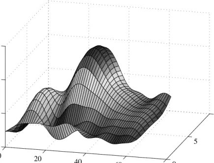
w(t) ∈ _C is the additive white Gaussian noise (AWGN) term, h ∈ _C is the channel impulse response (CIR), τmax is the maximum delay spread, t denotes time and τ is delay. Due to the movement of the mobile stations and multi-path propagation, the CIR has a two dimensional structure, as depicted in Fig. 2.1, where time t and delay

τ are normalized by symbol duration T and sampling interval Ts, respectively.

In wide-band communication systems, a wireless channel can be modeled by a tapped delay line with irregularly spaced tap delays. Each channel tap is the superposition of a large number of scattered plane waves that arrive with approximately the same delay. The wide-band channel has a time-variant impulse response, which can be written as

h(t, τ) = L

X

l=1

(14)

0 ₁ 2 ₃ 4 ₅ 0 5 10 0 0.1 0.2 0.3 0.4 0.5 t/T τ/T s |h|

Figure 2.1: Two dimensional structure of channel impulse response.

whereξ is the time-varying complex amplitude, Lis the total number of taps, l is the index tap and τl is the delay of thelth tap.

An important class of channels is widely used, where taps with different propagation delays are uncorrelated and the complex amplitude is a wide-sense stationary process. This class of channels is referred to as wide-sense stationary uncorrelated-scattering (WSSUS) channels. In WSSUS channels,ξl(t)’s are wide-sense stationary (WSS) com-plex Gaussian processes and independent for different taps with average powerσ2

l. The average power of each tap σ2

l is usually described by the power-delay profile (PDP) as shown in Fig. 2.2. Furthermore,ξl(t) is generally assumed to have the same correlation function rt(∆t). Hence

Rξlξl(∆t),E{ξl(t)ξ

∗

l(t+ ∆t)}=σl2rt(∆t), (2.3)

whereRξlξl is the auto-correlation function (ACF) ofξl, (·)

∗ _{is the complex conjugate.}

A special case of WSSUS model is often considered, where there is no line of sight (LoS) between the transmitter and receiver. The signal envelope follows a Rayleigh distribution, thus, this model is referred as Rayleigh fading. Using Clarkes’ isotropic scattering model [21], the temporal correlation function can be obtained as

(15)

2.2 Orthogonal frequency division multiplexing 0 5 10 15 20 −20 −15 −10 −5 0 τ/µs Fractional power (dB) Typical urban (a) 0 5 10 15 20 −20 −15 −10 −5 0 τ/µs Fractional power (dB) Bad urban (b) 0 5 10 15 20 −20 −15 −10 −5 0 τ/µs Fractional power (dB) Rural area (c) 0 5 10 15 20 −20 −15 −10 −5 0 τ/µs Fractional power (dB) Hilly terrain (d)

Figure 2.2: Power-delay profile for (a) typical urban, (b) bad urban, (c) rural area, (d) hilly terrain, from COST 207 [30]. The figures show the average power for each tap, normalized by the total power.

where J0(x) = ∞ P m=0 (−1)m m!Γ(m+1) x 2 2m

is the zero order Bessel function of the first kind,

fD is the maximum Doppler frequency. fD is associated with the carrier frequency fc and moving speed of the MS v by

fD =

v

cfc, (2.5)

where cis the speed of light.

2.2 Orthogonal frequency division multiplexing

In wide-band wireless communications, due to multipath propagation, the channel frequency response (CFR) is generally not flat. The frequency fluctuation causes erroneous Rx signal, which can be compensated with OFDM [53]. In OFDM, the transmission frequency band is divided into K equally spaced subbands, such that in each subband the frequency response is nearly flat.

(16)

0 ₂₀ 40 ₆₀ 80 0 5 10 0 0.5 1 1.5 n k |H|

Figure 2.3: Two dimensional structure of CFR corresponds to CIR in Figure 2.1

In practice, the Tx signal x is obtained by the inverse discrete Fourier transform (IDFT). The frequency domain discrete Tx signal can be written as

X[n, k] = K−1 X m=0 x(nT +mTs) exp{−2πkm∆f Ts} = K−1 X m=0 x(nT +mTs) exp −2πkm K , (2.6)

where n is discrete the time index and k is the subcarrier index. And the sampling interval Ts is defined as T /K. X[n, k] can be recovered at the Rx side by the discrete Fourier transform (DFT). IfK is a power of two, DFT and IDFT can be efficiently im-plemented using the fast Fourier transform (FFT). To avoid inter-carrier interference, the subcarrier spacing has to satisfy the orthogonality condition

∆f , 1

T. (2.7)

Suppose the delay taps are on the sampling grid with sampling rate Ts

(17)

2.2 Orthogonal frequency division multiplexing

the CFR of the kth subcarrier can be written as

H(t, k) = L X l=1 ξl(t) exp −2πkτl T (2.9) = L X l=1 ξl(t) exp −2πkl K , (2.10)

and the corresponding discrete CFR of the nth OFDM block can be written as

H[n, k] = L X l=1 ξl(nT) exp −2πkl K . (2.11)

The corresponding CFR of the CIR from Figure 2.1 with 64 subcarriers is shown in Figure 2.3, where it can be seen that the fluctuation within one subcarrier is much smaller than within the whole frequency band. This property leads to simplification of equalization. And it also enables radio resource allocation.

Consider time indices t1, t2 and subcarrier k1, k2, the correlation function of the CFR for different times and frequencies is

E{H(t1, k1)H∗(t2, k2)} = E ( _L X l=1 L X m=1 ξl(t1)ξm∗(t2) exp −2πk1l K exp 2πk2m K ) = rt(t2−t1) L X l=1 σ2 l exp −2π(k2−k1)l K = rt(∆t)rf[∆k], (2.12)

where ∆t = t2 −t1, ∆k = k2 −k1 and rf[∆k] is the discrete frequency correlation function, defined as rf[∆k], L X l=1 σ2 l exp −2π∆kl K . (2.13)

From (2.12), it is clear that the correlation in time and frequency domain can be decoupled, and the frequency correlation depends on the PDP.

Moreover, OFDM can be extended to multiple users, with each user using a subset of the subbands. This multiple access scheme is called orthogonal frequency divi-sion multiple access (OFDMA). Due to their unique advantages, OFDM and OFDMA are adopted for many industrial standards, such as LTE, wireless local area network (WLAN) and digital video broadcasting - terrestrial (DVB-T). Thus, in the foreseeable future, OFDM and OFDMA will be the dominant technology in wireless communica-tions.

(18)

Figure 2.4: MIMO channel

2.3 Multi-antenna transmission

Another trend in wireless communications is MIMO transmission. Using multiple Tx and Rx antennas, the energy efficiency and spectral efficiency can be improved significantly [31] [83]. Consider a MIMO channel with NTx Tx antennas and NRx Rx antennas, as shown in Figure 2.4, the wireless channel can be expressed in matrix form

Ht(t, τ) =      h1,1(t, τ) h1,2(t, τ) · · · h1,NTx(t, τ) h2,1(t, τ) h2,2(t, τ) · · · h2,NTx(t, τ) .. . ... . .. ... hNRx,1(t, τ) hNRx,2(t, τ) · · · hNRx,NTx(t, τ)      , (2.14)

where hnRx,nTx represents the channel between the nRxth Rx antenna and nTxth Tx antenna. Similar to (2.1), the received symbols can be described in the vector form:

yt(t) = τmax Z 0 Ht(t, τ)xt(t−τ)dτ +wt(t), (2.15) with yt(t) =      y1(t) y2(t) .. . yNRx(t)      ,xt(t) =      x1(t) x2(t) .. . xNTx(t)      ,wt(t) =      W1(t) W2(t) .. . WNRx(t)      (2.16)

being the Rx symbol vector, Tx symbol vector and AWGN vector, respectively. Although the energy and spectral efficiency can be improved by using multiple anten-nas, for wide-band MIMO transmission with larger numbers of antenanten-nas, the equal-ization problem can become increasingly difficult. Therefore, OFDM and MIMO tech-niques are often combined into MIMO-OFDM systems, in which the CFR is quasi-constant for each subband, and equalization can be done in the frequency domain [93].

(19)

2.4 Cellular networks

Using (2.6) and (2.11), the received signal vector in frequency domain can be written as

yf[n, k] =Hf[n, k]xf[n, k] +wf[n, k], (2.17) whereyf,xf wf are vectors collecting the frequency domain Rx, Tx signals and AWGN, respectively. Elements of CFR matrix Hf are the IDFT of Ht as defined in (2.11). In addition to the two dimensional structure described in Figure 2.3, MIMO-OFDM channels have the third dimension of space. The spatial correlation can degrade the channel capacity [47], thus, should be properly described. Models for spatial correlation are elaborated in Chapter 3.

2.4 Cellular networks

Cellular networks are one of the most widely deployed wireless communication net-works. Figure 2.5 shows the common layout of a cellular network. Typically, a cellular network consists a number of BSs and a big amount of MSs. The behavior of the network depends on many facts, such as the distribution, movement and service types of the MSs, the antenna tilts, Tx power of the BSs, etc. Theoretical analysis of such complex system is usually very difficult, thus, computer simulation is quite commonly used. Moreover, due to the large amount of entities in the network, simulation of the network level cannot cover all the phenomena in the communication links. A higher level of abstraction is desirable.

In link level modeling, the wireless channel is characterized by the relative location and velocity of the user, number and orientations of the antennas, frequency and bandwidth of the signal, as well as the propagation environment. In network level modeling, all the factors that affect the channel condition are translated into a measure of CSI. Furthermore, in a multi-cell network, the CSI takes also the interferences from neighboring cells into consideration. Signal to interference plus noise ratio (SINR) is a common measure of the CSI. For an OFDM system, the SINR of user i served by base station s at timet and subcarrier k can be written as

γi,s(t, k) = Pi,s(t, k) P j∈S\s Pi,j(t, k) +σ2w , (2.18)

whereP is the Rx power and σ2

w is the noise power, S is the set of all the cells within the network.

Theoretically, the CSI should be given as input to the cellular network control entities. However, in practice, this information is typically unavailable at the BS and must be provided by the MS periodically through a feedback channel. From the aforementioned wireless communication links, a dilemma arises. On one hand, due to the doubly selectivity of the channel, optimizing the cellular network requires as much and as detailed information as possible. And on the other hand, a large amount of feedback information leads to a large packet overhead, which deteriorates the spectral efficiency.

(20)

x position [m] y position [m] 200 400 600 800 1000 1200 1400 1600 200 400 600 800 1000 1200 1400 1600

Figure 2.5: Rx signal level of a network with 7 base stations and 21 cells in hexagonal layout, where the basestations are located on the joints of the hexagonal cells

In the current LTE standards, the CSI is compressed for different subcarrier before the feedback process. The influence of CSI feedback is elaborated in Chapter 4. With the CSI available at the BS, the cellular network can be optimized through network control strategies, such as radio resource allocation, handover optimization, antenna tilt and Tx power management, etc.

2.5 3GPP LTE

An important part of this thesis are physical layer downlink control strategies based on the user reported CSI, especially with application to LTE systems.

To comply with the standards, some LTE terminologies are used in this thesis, e.g. the base stations is called evolved node B (eNB) and the mobile station is called user equipment (UE).

2.5.1 System architecture

Comparing with older generations, LTE does not only offer a new radio interface but also a new system architecture. 3GPP specifies the system architecture evolution (SAE) in Release 8. As an all-IP system, there is no more circuit switching center

(21)

2.5 3GPP LTE

Figure 2.6: LTE system architecture

in LTE. To reduce latency, the architecture of LTE is flatter than of older systems. Especially for the user plane (UP), data can be directly passed from BSs to gateways without going through a control entity [39].

The network architecture of LTE is illustrated in Figure 2.6, where the UE is connected to some eNB via evolved universal terrestrial radio access (E-UTRAN). In the user plane, data is sent to some serving gateway (S-GW), which is the mobile anchor point. The S-GW is in charge of inter-eNB handover, downlink packet buffering, initiation of network-triggered service requests, etc. The S-GW is connected to a PDN gateway (P-GW), where the IP address of UE is allocated. Through the P-GW, the data finally reaches the core network.

In the control plane, the mobility management entity (MME) is the main control unit. Main functions of the MME include authentication and mobility management. Basically, MME is a server identifies the UE, request proper resources in the eNB for the UE and decides which S-GW the UE is connected to. To engage authentication and mobility management functions, the MME has to request subscription data from the home subscription server (HSS), which is a repository for all permanent user data.

2.5.2 Physical layer transmission

In the LTE downlink, user data is transmitted via the physical downlink shared channel (PDSCH) and control information is transmitted via the physical downlink control channel (PDCCH). The following procedure is applied to the downlink user data [11]: Transport Block Cyclic redundancy check (CRC) Attachment: A 24-bit CRC mes-sage of the whole transport block is calculated and attached, where CRC is for error detection at the Rx side.

Code Block Segmentation and Code Block CRC Attachment: The transport block attached with CRC bits is chopped up in to smaller blocks and each block is attached with another 24-bit CRC. To fit into the turbo interleaver, the minimum and maximum block size is 40 bits and 6144 bits including the CRC bits, respectively. Moreover, filler bits are appended to the start of the first segment to match the turbo interleaver. Turbo Encoding: Turbo coding is applied to each segment to enhance error performance [17]. The turbo encoder is a parallel concatenated convolutional code (PCCC) with two recursive convolutional encoders and a quadratic permutation polynomial (QPP) interleaver [65].

(22)

Figure 2.7: LTE downlink signal generation

Rate Matching: The encoded streams are further processed by a rate matching algo-rithm. Together with the turbo encoder, the rate matching algorithm is capable of producing any arbitrary rate to match for the transmission resources [20].

Code Block Concatenation: The output blocks of rate matching are sequentially con-catenated to create the final output of channel coding.

Scrambling: The codewords are bit-wise multiplied by an orthogonal sequence and a user-specific pseudo-random scrambling sequence. The purpose of scrambling is to suppress inter-cell interference (ICI). Since the scrambling sequence is pseudo-random and user-specific, signals from interfering cells can not be descramble correctly. The result is an uncorrelated, noise-like sequence.

Modulation Mapping: The scrambled codewords are modulated to complex valued symbols with quadrature phase shift keying (QPSK), 16-quadrature amplitude

(23)

modu-2.5 3GPP LTE

lation (QAM) or 64-QAM. The modulation scheme is chosen to adapt to the channel condition.

Layer Mapping and Precoding: Since MIMO transmission is adopted in LTE, the com-plex symbols are mapped onto 1, 2 or 4 spatial layers and multiplied with the precoding matrix, depending on the number of Tx antennas. For single antenna transmission, layer mapping and precoding is a dummy process with the output equal to the input. For multiple Tx antennas, the mapping and precoding scheme depends on the number of antennas as well as the MIMO transmission mode, which can be either transmit diversity or spatial multiplexing.

Resource Element Mapping: A Resource Element (RE) is the smallest defined unit which consists of one OFDM sub-carrier during one OFDM symbol interval. For each antenna port, the resource elements which are not occupied by other control channels can be used for PDSCH. The symbols are mapped sequentially to the available resource elements from the first to the last subcarrier in the first OFDM symbol, and this process goes on in the remaining OFDM symbols until there is no symbol left.

OFDM Signal Generation: With the resource elements filled with data symbols, OFDM signal can be generated with inverse fast Fourier transform (IFFT).

The whole procedure is summarized in Figure 2.7 and more details can be found in [6].

(24)

(25)

3 Link Level Modeling

This chapter introduces link level modeling, especially for MIMO transmission. As the fundamental part of characterizing wireless communication systems, channel models can be categorized into analytical models and geometry-based models. Analytical models emphasize correlation properties, whereas the geometry-based models try to describe the influence of the spatial environment on the radio wave.

Furthermore, geometry-based models can be divided into deterministic models and stochastic models. Moreover, a semi-stochastic model, which is a hybrid of the deter-ministic and stochastic model, is also presented in this chapter.

Parts of this chapter have been published in [97],[93], [101], [98], [102] and [19].

3.1 Analytical models

Analytical MIMO channel models specify channel matrices which have correct relation properties, generated from basic random number generators. Since the cor-relation functions of the CFR can be decoupled, the procedure of generating channel matrices for MIMO-OFDM systems can be divided into three steps [90]. The first step is to generate independent Rayleigh processes with temporal correlation. The second step is to apply power delay profile (PDP). And the last step is to create a channel matrix with spatial correlation.

3.1.1 Rayleigh fading process

In the ideal case, the CIRs for different Tx-Rx antenna pairs of a MIMO system are independent and identically distributed (i.i.d.). Each channel between antenna pairs can be regarded as a single-input single-output (SISO) channel. This model is also referred to as the i.i.d. model. The generation of i.i.d. channels is rather straight forward. A Rayleigh flat fading CIR with unit variance ζl is generated for each of the

L taps, and then scaled with the varianceσ2

l specified in the PDP.

Many different techniques have been proposed to model and simulate mobile radio channels with Rayleigh fading. The most representative models from early years are from Clarke and Gans based on sum of sinusoids [21] [33]. In Clarke’s reference model, the electro-magnetic field of the received signal is assumed to be comprised of a number of sinusoidal plane waves with equal average amplitude and different Doppler frequency shifts. The angle of arrivals (AoAs) and phases of these waves are arbitrary [70].

(26)

Accordingly, the normalized complex envelope of an arbitrary propagation path l can be written as ζl(t) = 1 √ Nsin Nsin X nsin=1

exp{(2πfDtcosψl,nsin+ Φl,nsin)}, (3.1)

whereNsinis the number of sinusoids,nsin is the index of sinusoidal wave,ψ is the ran-dom AoA and Φ is the ranran-dom initial phase. Bothψ and Φ are uniformly distributed over [−π, π) for allnsin, and they are mutually independent. From the Euler’s formula, (3.1) can be expressed with the in-phase and quadrature components

ζl(t) = ζI,l(t) +ζQ,l(t), (3.2)

where the in-phase and quadrature components are given by

ζI,l(t) = √1

Nsin Nsin

X

nsin=1

cos (2πfDtcosψl,nsin+ Φl,nsin) (3.3)

ζQ,l(t) = √1

Nsin Nsin

X

nsin=1

sin (2πfDtcosψl,nsin+ Φl,nsin). (3.4)

For large Nsin, the central limit theorem justifies that ζI,l(t) andζQ,l(t) can be treated as Gaussian random processes. When Nsin approaches infinity, the autocorrelation of

ζl is [81]

Rζlζl(∆t) = E{ζl(t1)ζ

∗

l(t2)}

= E{(ζI,l(t1) +ζQ,l(t1))(ζI,l(t2)−ζQ,l(t2))}

= RζIζI(∆t) +RζQζQ(∆t) +(RζQζI(∆t)−RζIζQ(∆t)), (3.5)

where

RζIζI(∆t) =RζQζQ(∆t) = 1

2J0(2πfD∆t) (3.6)

(27)

The first part of (3.6) can be proved as follows:

RζIζI(∆t) = E{ζI(t1)ζI(t2)} = 1 Nsin Nsin X nsin=1 Nsin X msin=1

Eψ,Φ{cos (2πfDt1cosψl,nsin+ Φl,nsin)

·cos (2πfDt2cosψl,msin+ Φl,msin)}

= 1

2Nsin Nsin

X

nsin=1

{Eψ{cos(2πfD(t1−t2) cosψl,nsin)}

+Eψ{cos(2πfD(t1+t2) cosψl,nsin)}EΦ{cos 2Φl,nsin} +Eψ{sin(2πfD(t1+t2) cosψl,nsin)}EΦ{sin 2Φl,nsin}}

= 1

2Nsin Nsin

X

nsin=1

Eψ{cos(2πfD∆tcosψl,nsin)}

= 1 2Nsin Nsin X nsin=1 Z π −π

cos(2πfD∆tcosψl,nsin)

dψl,nsin 2π = 1 2Nsin Nsin X nsin=1 J0(2πfD∆t) = 1 2J0(2πfD∆t). (3.8)

Similarly, the second part of (3.6) and (3.7) can be proved.

Based on Clarke’s reference model, Jakes proposed a simplified simulation model, which has been widely used for decades [45]. In the Jakes’ model, the AoA and initial phase are set to

ψJakes,l,nsin =

2πnsin

Nsin

, (3.9)

ΦJakes,l,nsin = 0, (3.10)

and Nsin is taken from

Nsin= 4Msin+ 2. (3.11)

where Msin is an integer. The value of Msin determines the number of summed sinu-soids, and thus the statistical property of the model.

Jake’s model reduces the number of distinct Doppler frequency shifts from Nsin to

Msin + 1. However, the deterministic nature of the Jakes’ simulation model makes it difficult to create multiple uncorrelated fading waveforms for frequency selective channels.

A randomized simulator, which can solve this problem, is proposed by Pop and Beaulieu [69]. Pop and Beaulieu’s simulation model also solves the stationarity prob-lem of Jakes’ model, but higher-order statistics of this model do not match the desired

(28)

ones [104]. This deficiency can be overcome by introducing randomness in path gain, initial phase and Doppler frequency for all individual sinusoids. In [91]. Xiao et al. introduced a simulation model following the principles of Clarke’s reference model

ζXiao,l(t) = ζXiao,I,l(t) +ζXiao,Q,l(t) (3.12)

ζXiao,I,l(t) = 1 √ Nsin Nsin X nsin=1

cos (2πfDtcosψXiao,l,nsin+ ΦXiao,l,nsin) (3.13)

ζXiao,Q,l(t) = 1 √ Nsin Nsin X nsin=1

sin (2πfDtcosψXiao,l,nsin+ ΦXiao,l,nsin), (3.14)

with the AoA generated by

ψXiao,l,nsin =

2πnsin+θl,nsin

Nsin

, (3.15)

whereθl,nsin and ΦXiao,l,nsin are statistically independent and uniformly distributed over [−π, π) for all l and nsin.

For systems with L delay taps, NTx Tx antennas and NRx Rx antennas, in total

LNTxNRx Rayleigh processes must be independently generated, with the underlying assumption that the normalized temporal correlation function is identical for all re-solvable physical multipaths.

Other than sum of sinusoids, IDFT and autoregressive (AR) models are also proposed to create Rayleigh processes [103] [13]. IDFT and AR models have the advantage in computational complexity, however, both of them have limitations on applications. The IDFT method can only work with a relatively large Doppler frequency and FFT size. Whereas AR models have severe numerical problems when the Doppler frequency is small.

Assuming the PDP is identical for all Tx and Rx indices [59], σ2

l can be applied to each delay tapl

hi.i.d.(t, τ) = L

X

l=1

σlζl(t)δ(τ−τl), (3.16) where the relation between σl and τl is generally given in tables from the PDP. For various wireless networks, specific PDP can be found in many standards [30] [40] [3]. The channel matrix Hiid(t, τ)∈CNRx×NTx simply collects the CIRs, and arrange them in an appropriate order.

3.1.2 Kronecker model

The i.i.d. model is mostly favored by theoreticians, due to its mathematical tractabil-ity. However, spatial correlation of MIMO channels should not be ignored in the general case, since it has a large impact on the channel capacity [79].

(29)

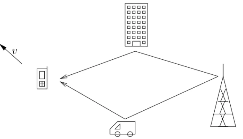
v

Figure 3.1: Multi-path propagation and movements of mobile station cause frequency selective time varying fading.

Assuming the spatial correlations are identical for all resolvable physical multipaths, and static over time, the time and delay indices can be dropped. For arbitrary time and delay, the spatial correlation matrix RH∈CNRxNTx×NRxNTx is defined by

RH,E{vec(Ht)vec(Ht)H}, (3.17) where vec(Ht) = [h1,1, h2,1,· · · , hNRx,1, h1,2,· · · , hNRx,2,· · · , hNRx,N T x]T and Ht is de-fined in (2.14). The operators (·)T _{and (}_·₎H _{are the matrix transpose and Hermitian} transpose, respectively. The correlation matrix is symmetric and real valued on its diagonal.

If the correlation matrix is known, a spatially correlated channel matrix Hcorr can be generated from the i.i.d. channel matrix in a rather straight forward way.

Hcorr = unvec(R 1/2

H vec(Hiid)) (3.18)

whereR1/2_H is the square root of RH, unvec(·) is the inverse operation of vec. R 1/2 H has to be computed by solving the equation

R1/2_H (R1/2_H )H=RH. (3.19) In generalRH is positive definite, thus,R

1/2

H can be computed by its Cholesky decom-position [78].

One of the drawbacks of the full correlation matrix is its big size. It needs (NRxNTx)2 parameters to be fully specified. Furthermore, a direct interpretation of RH with respect to the physical propagation of radio channel is difficult.

A simplification of the full correlation matrix approach is proposed in [50], where all antenna elements in both antenna arrays are assumed to have the same polarization and radiation pattern. In addition, all elements on the transmitter and receiver side obtain the same power azimuth spectrum (PAS) from each element on the opposite side. The full channel spatial correlation matrix RH can be written as

RH = 1 tr{RRx}

(30)

where ⊗ denotes the Kronecker product and tr(·) is the matrix trace. The one side Tx and Rx correlation matrices are defined as

RRx = E{HtHHt} (3.21)

RTx = E{HHtHt}, (3.22)

respectively. And the spatially correlated channel matrix can be generated using Hkron = 1 p tr{RRx} R1/2_RxHiid(R 1/2 Tx) T_, _(3.23)

where R1/2_Rx and R1/2_Tx can be calculated using Denman-Beavers square root iteration [79]. The number of parameters required to fully characterize the MIMO channel by the Kronecker model is N2

Tx +NRx2 , which is significantly smaller than by the full correlation model.

Generally, the modeling parametersRRx andRTx should be estimated using measure-ment data. Moreover, a further simplification of the Kronecker model is proposed in [86], where only one coefficient is required to represent the Tx or Rx correlation ma-trix. The single coefficient Kronecker model is idealistic, however very easy to apply, thus, quite often used in scientific researches.

3.1.3 Weichselberger model

By assuming the separability of both link ends, the Kronecker model decomposes the full correlation matrix into Tx and Rx correlation matrices, and thus offers simplicity for theoretical analysis. However, the ignored joint correlation properties at the trans-mitter and receiver lead to an underestimation of channel capacity with Kronecker model [68].

Consider the case that both link ends are not independent, the one-sided correlation matrices have to be parameterized by the statistical properties of the other link end

RRx,QTx = E{HtQTxH H t} (3.24) RTx,QRx = E{H H tQRxHt} (3.25)

whereQTx and QRx are the spatial signal covariance matrices of the Tx and Rx sides, respectively [87]. The Kronecker model is a special case where QTx and QRx are identity matrices.

It is easy to prove that both RRx,QTx andRTx,QRx are normal matrices. They can be factorized using the eigenvalue decomposition as

RRx,QTx = URxΛRx,QTxU H Rx (3.26) RTx,QRx = UTxΛTx,QRxU H Tx, (3.27)

where Λ are real-valued diagonal matrices with nonnegative entries. The eigenbases URx and UTx do not have dependencies on the correlation of the other link end.

(31)

3.2 Deterministic models Tx (b) Tx Rx (a)

Figure 3.2: Deterministic channel models: (a) Ray-tracing; (b)Ray-launching. The channel matrix of Weichselberger model can be written as

Hweich =URx e ΩHiid UT_Tx, (3.28)

where ˜Ω is the element-wise square root of the power coupling matrix Ω, is the element-wise matrix product.

The modeling parameters RRx,QTx, RTx,QRx and Ω must be extracted from measure-ment data, in order to recreate a certain channel condition. Detailed information is given in [87]. By considering the joint correlation on both link ends, the average mu-tual information of the channels generated by the Weichselberger model matches the measurements quite well, while the Kronecker model tends to underestimate the chan-nel capacity [67]. However, since the model parameters can only be estimated from measurement data, the Weichselberger model is not applicable for a given environment without a measurement campaign.

3.2 Deterministic models

Unlike the analytical models, the starting point of geometry-based models is the phys-ical wave propagation. According to the modeling methodology, geometry-based mod-els can be categorized into deterministic modmod-els and stochastic modmod-els.

Deterministic models, such as ray-tracing and ray launching, characterize the physical propagation parameters in a completely deterministic manner by following or launch-ing deflected rays from transmitters to receivers [89] [54]. In deterministic models, electromagnetic characteristics of radio links are explicitly calculated by means of a detailed description of the propagation environment. Deterministic models capture the nature of radio wave propagation, thus are intuitive and potentially accurate. However, they are site specific, i.e., geometric information about the propagation environment must be known.

In deterministic models, all possible paths from the Tx to the Rx are determined by considering propagation phenomena like reflections at walls and diffractions at

(32)

building edges. Usually, the propagation environment is described by polyhedrons. A visibility tree is build to capture the radio propagation paths. The visibility tree consists of nodes and branches, representing objects (walls, wedges, Rx, etc.) and LoS connections between objects, respectively. The layered structure of the visibility tree represents the depth of interactions.

For ray-tracing, the images of Tx relative to the reflecting planes are computed, as depicted in Figure 3.2 (a). Each reflected or diffracted ray from the Tx to the Rx is exactly determined. This calculation leads to a very high accuracy, because all the relevant objects are always considered for the selection of interactions. However, as the number of interactions increases, the computational complexity grows exponentially. With ray-launching, the rays are launched from the transmitter homogeneously with a discrete angle increment [89]. After each interaction, the reflected or diffracted rays are computed and traced further as illustrated in Figure 3.2 (b). The tracing can be terminated, when the power of a ray drops under a predetermined threshold. The disadvantage is that the constant increment between two rays leads to the problem that it is hard to determine whether a wedge is hit or not.

Despite the high accuracy, the computational burden makes ray-tracing incapable of handling large wireless communication scenarios [85]. Thus, it is mostly used for in-door or microcell environment. The ray-launching method has many advantages in predicting field strength for a large area [61]. In urban scenarios, a cube oriented 3D ray launching algorithm (CORLA) proposed in [58] offers both fast and accurate field strength prediction. As an enhancement of CORLA, the ray-launching tool par-allel implemented ray optical prediction algorithm (PIROPA) benefits from parpar-allel computing peripherals, and thus provides an even faster solution [74].

However, since CORLA, PIROPA and other ray-tracing/launching algorithms are to-tally deterministic, they are generally used to predict field strength but not to generate channel matrices.

3.3 Geometry-based stochastic channel models

During radio wave propagation, a transmitted signal can be reflected or diffracted by various scatterers. In geometry-based stochastic channel model (GSCM), with geomet-rical description of the propagation environment (e.g. urban, suburban, etc.), locations of the scatterers are chosen randomly. After that, statistical information about the ra-dio wave is generated and superimposed to create channel matrices. Moreover, for the purpose of creating an easy-to-use solution to conduct simulations, a few standardized GSCMs have been proposed.

3.3.1 Double directional channel model

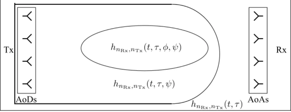
To generate the statistical information, the influence of various elements on the radio channel should be studied separately. Consider the Rx side, the Rx antennas

(33)

coher-3.3 Geometry-based stochastic channel models

Figure 3.3: The relationship among the radio channel, the single directional channel and the double directional channel.

ently collect the components from all directions, and weight them with the directional antenna gain hnRx,nTx(t, τ) = Z ψ p GnRx(ψ)hnRx,nTx(t, τ, ψ)dψ, (3.29) where the single directional channel impulse response (CIR) hnRx,nTx(t, τ, ψ) is param-eterized by the angle of arrival (AoA). The directional Rx antenna gain GnRx depends on the antenna geometry and orientation.

Moreover, the Tx antennas distribute the signal energy into the desired angle of depar-ture (AoD), the single directional CIR is the integration over all angles of depardepar-ture AoDs hnRx,nTx(t, τ, ψ) = Z φ p GnTx(φ)hnRx,nTx(t, τ, φ, ψ)dφ, (3.30) where GnTx is the Tx antenna gain.

To summarize, the CIR is a function of the double directional CIR:

hnRx,nTx(t, τ) = Z φ Z ψ p GnTx(φ) p GnRx(ψ)hnRx,nTx(t, τ, φ, ψ)dφdψ. (3.31)

The relationship of the CIR, the single directional CIR and the double directional CIR is shown in Figure 3.3. Clearly, the double directional channel model divides the radio channel into three parts: Tx antennas, Rx antennas and the double directional channel in between. In [80], the double directional channel model is validated with measurement data, laying the foundation of standardized GSCMs.

3.3.2 Multi-path component clusterization

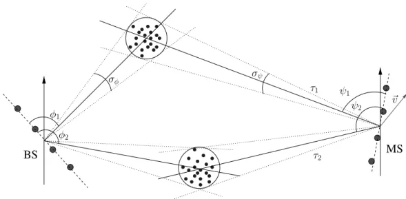
In principle, the double directional channel model is an integral of multi-path com-ponents (MPCs), which has a distinct set of propagation parameters, such as AoD, AoA and delay. However, measurements show that these MPCs are often observed in clusters, where a cluster is a group of MPCs with similar propagation parameters as

(34)

Figure 3.4: Clusterized multi-path MIMO channel model

shown in Figure 3.4 [71]. Ignoring the clustering effects results in overestimation of the channel capacity [52].

To engage computer-based simulation, the double directional channel model must be discretized. Therefore, the CIR of a cluster can be represented by the summation of a discrete number of MPCs.

The MIMO CIR can be written as

hnRx,nTx(t, τ) = Nc X nc=1 NM X nM=1 q GnTx(φnc,nM) q GnRx(ψnc,nM) ·hnRx,nTx,nc,nM(t, τnc,nM, φnc,nM, ψnc,nM) (3.32) where nc and nM are the index of cluster and index of MPC within a cluster, respec-tively. And Nc and NM are the number of clusters and number of MPCs within a cluster, respectively.

Due to the similarity of the AoDs, AoAs within a cluster, they can be modeled as the cluster parameters with a small offset value [26]:

φnc,nM =φnc +AoD,nM (3.33)

ψnc,nM =ψnc+AoA,nM, (3.34) where AoD,nM and AoD,nM are the offset values of AoD and AoA, respectively.

3.3.3 Standardized models

In the double directional channel model, the antenna geometry can be designed to produce desirable antenna patterns. The angularly resolved double directional CIRs can be generated, if their statistical properties are known. Following this concept,

(35)

3.3 Geometry-based stochastic channel models

standardized simulation models, such as 3GPP spatial channel model (SCM) [4], 3GPP spatial channel model extension (SCME) [15] and wireless world initiative new radio (WINNER) model [44], have been developed. Standardized models enable their users to generate channel matrices without performing measurement campaigns.

To develop standardized models, the standardization entities first have to conduct a large amount of channel measurements. The measured data are then analyzed and the statistical parameters are extracted. Supposedly, these models are able to recreate wireless channels with the same statistical behavior.

To use a standardized model, people have to choose a scenario (Urban, suburban, rural area, etc.) and set up the network layout as well as antenna parameters. With these settings given, the model first generates large scale parameters (LSPs), e.g., AoD spread, AoA spread and delay spread. Basically, the LSPs specify statistical properties of the small scale parameters including AoD, AoA, delay, etc. With the specified statistical properties, small scale parameters can be randomly generated and the channel coefficients can be calculated accordingly.

The generation of channel coefficients follows a generic model. Taking the scenario described in Figure 3.4 as an example, where both the Tx and Rx antenna arrays are uniform linear arrays (ULAs). Assuming that in each cluster, the power is uniformly distributed for every MPC, the CIR can be written as

hnRx,nTx(t, τ) = Nc X nc=1 p Unc,nM NM X nM=1 q GnTx(φnc,nM) q GnRx(ψnc,nM) ·exp  2π λ k T Tx,nc,nMdTx,nTx + Φnc,nM ·exp 2π λ k T Rx,nc,nMdRx,nRx ·exp 2π λ vnc,nMt δ(τ −τnc,nM), (3.35) whereUnc,NM is the MPC power. It is common to assume the cluster power is uniformly distributed in each MPC:

Unc,nM =

Unc

NM

. (3.36)

The wavelength of the carrier wave is denoted by λ. Φnc,nM is a random initial phase and τnc,nM is the path delay. The directional vectors are defined as [92]

kTx,nc,nM = cosφnc,nM sinφnc,nM , kRx,nc,nM = cosψnc,nM sinψnc,nM , (3.37)

whereφnc,nM and ψnc,nM are generated with a cluster AoDφnc and AoAψnc plus path specific offset angles. Furthermore, the AoDs and AoAs are randomly coupled. The position vectors are defined as

dTx,nTx = xTx,nTx yTx,nTx , dRx,nRx = xRx,nRx yRx,nRx , (3.38)

(36)

0 0.5 1 1.5 2 2.5 3 3.5 x 10−6 −90 −80 −70 −60 −50 −40 −30 −20 −10 0 Delay [s] Normalized power [dB]

Semi−stochastic model NLOS

(a) 0 0.5 1 1.5 2 x 10−6 −30 −25 −20 −15 −10 −5 Delay [s] Normalized power [dB]

WINNER model C2 NLOS

(b)

Figure 3.5: Power-delay profiles for a NLoS environment in (a) Semi-stochastic channel model (b) WINNER model C2 scenario (typical urban macrocell)

wherexTx,nTx, yTx,nTx, xRx,nRx, yRx,nRx are X and Y coordinates of thenTxth Tx antenna element and nRxth Rx antenna element, respectively. And the Doppler frequency component is defined as

vnc,nM =vcos(ψnc,nM −ϑ) (3.39) where v and ϑ are speed and angle of the movement of the user, respectively.

There are some further extensions of this generic model including LoS support, polar-ized antenna, elevation angles, etc.

Among these three standardized models, the WINNER model provides the widest range of carrier frequency and bandwidth, the largest set of scenarios, and cross-correlation among LSPs. The WINNER model also allows a discrete time evolution of simulation parameters. Therefore, the WINNER model can be regarded as the leading MIMO channel model among existing standardized models [62].

3.4 Semi-stochastic channel model

In the WINNER model, the total number of different scenarios is 17, which is signif-icantly larger than the 3 scenarios specified in SCM and SCME. However, there are still limitations for the standardized GSCM. Although some stochastic characteristics of the wireless channel are preserved, location specific geographical data can not be utilized to improve modeling accuracy. For example, the terrain of the city Budapest is flat on the side of Pest and uneven on the side of Buda. However, with GSCM, one can only choose “Urban” scenario to simulate both areas, and neglect the definite differences between the propagation environments.

In contrastt, geographical information can be effectively utilized in the deterministic models. However, the conventional deterministic models only focused on predicting

(37)

3.4 Semi-stochastic channel model

field strength, taking neither the frequency selectivity caused by multi-path propa-gation nor spatial diversity caused by multiple antennas into consideration. In [74], the ray-launching tool PIROPA provides not only field strength but also multi-path information, e.g., AoA, AoD and the delay of each path. With the multi-path informa-tion, a semi-stochastic channel model (SSCM) can be applied to generate the channel coefficients [101].

3.4.1 Combining deterministic model and stochastic model

The central idea of SSCM is to replace the randomly generated cluster parameters with explicitly calculated ones. Thus, the advantages of deterministic model and GSCM can be combined. Figure 3.5 shows two power delay profiles used in SSCM and WINNER, respectively. Be aware that unlike in WINNER model, in SSCM, the PDP is calculated with the environment data and thus location based. Therefore, even in a single scenario setup, two different locations close to each other can have significantly different PDPs due to radio wave propagation.

The basic assumption of SSCM is the equivalence of propagation paths in PIROPA and clusters in GSCM. With this assumption, φnc and ψnc can be obtained from the output of PIROPA, andφnc,nM and ψnc,nM can be generated in the same way as in the standardized GSCMs.

The modeling procedure of SSCM can be summarized into two stages. The first stage is the deterministic stage, where PIROPA is performed on a certain city map. With the location of the BS and propagation environment given, PIROPA calculates propagation paths for every possible location of the MS on the map. The output information of this stage is totally deterministic. Therefore, for a given map, the deterministic stage is only needed to be performed once. The result can be saved into a file for the second stage. The second stage is the stochastic stage, where randomness is generated. In this stage, antenna patterns are applied according to antenna orientations; MPC parameters are generated following the same rules as described in the GSCMs and the Doppler frequency components are calculated for given moving speeds of the MSs. And finally (3.35) is used to calculate the CIR. In Table 3.1, the parameters generated in both stages are summarized.

3.4.2 Model validation

To validate the SSCM, MIMO data from a measurement campaign in Ilmenau is used for comparison.

Ilmenau measurements

The measurement campaign was done in July, 2008, in Ilmenau, a town in Thuringia, Germany. Ilmenau has a typical landscape of an European small to mid-sized town.

(38)

Deterministic stage Stochastic stage Nc NM Unc Unc,nM φnc φnc,nM ψnc ψnc,nM τnc τnc,nM dTx,nTx,dRx,nRx vnc,nM Φnc,nM

Table 3.1: Parameters for deterministic stage and stochastic stage

The terrain is not totally flat but without steep slopes. Most of the buildings have similar heights. These facts make Ilmenau an ideal place to test for the urban macro cell reference scenario.

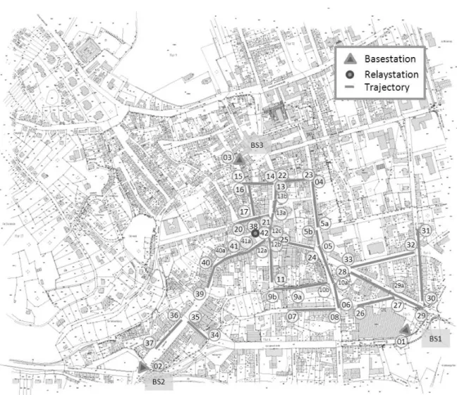
In the measurement campaign, three transmitters were placed on cranes and lifted to 25 meters above the ground to simulate BSs. Channel sounding equipments are carried by a car and traveled along 22 different trajectories, as shown in Figure 3.6. The campaign setup complies with 3GPP LTE standards. A pair of 40 MHz band at 2.53 GHz were measured [73]. On the BS side, a 8×1 polarized uniform linear patch array (PULPA) with beam width of 100◦ azimuth and 24◦ elevation is deployed. On the MS side, a 12×2 stacked polarimetric uniform circular patch array (SPUCPA) with omnidirectional azimuth pattern and 80◦ elevation beam width is adopted. The MS travels with a walking speed. The channel response is collected in frequency domain, as shown in Figure 3.7. Some of the measurement parameters are summarized in Table 3.2. Inter-site distance BS1-BS2 = 680m, BS2-BS3 = 580m, BS1-BS3 = 640m Tx power 46 dBm Center frequency 2.53 GHz Bandwidth 2×40 MHz CIR length 6.4 µs

CIR sampling 641 samples

Snapshot rate >75 Hz Positioning Odometer and GPS

(39)

Figure 3.6: Overview of Ilmenau measurement campaign Metric

For a wireless communication channel, the most important metric is the channel ca-pacity. For simplicity, consider the frequency domain model in (2.17). For a channel realization Hf, the mutual information is given by

I = log₂det INRx+HfQHHf

, (3.40)

where Q is the frequency domain spatial signal covariance matrix, defined as

Q= E(xf−E{xf})(xf−E{xf})H . (3.41) For fading channel with perfect CSI available at both the Tx and Rx ends, the ergodic channel capacity can be written as [36]

Cperfect = E max Q log2det INRx+ρTxHfQH H f , (3.42)

(40)

Figure 3.7: Measured CFR of path 9a-9b from Ilmenau data

whereρTxis the transmit signal to noise ratio (SNR). In this case, the channel capacity can be achieved if the transmit power is optimized with water filling.

If CSI is not available, the optimal covariance matrix Q is given by [83] Q= 1

NTx

INTx (3.43)

and the ergodic capacity becomes

Cno = E log₂det INRx+ ρTx NTx HfHHf . (3.44) Numerical results

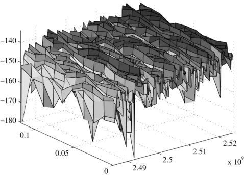
In the numerical evaluation,Cnocalculated for the SSCM and WINNER model is com-pared with the ergodic capacity obtained from measurements. For WINNER model, the same relative locations of the basestations and mobile stations are used. However, due to the limitation of GSCM, the location information of the buildings can not be given as input to improve the performance.

As shown in Figure 3.8, the ergodic capacity calculated by SSCM is very close to the measurements, whereas the WINNER model gives a more fluctuated result with much less accuracy. Therefore, the extra geographic information provided to the ray

(41)

3.4 Semi-stochastic channel model 20 40 60 80 100 120 5 6 7 8 9 10 11 12 Frequency range [MHz] Capacity [bits/s/Hz]

WINNER II channel model Semi−stochastic channel model Ilmenau data

Figure 3.8: Ergodic channel capacity for path 9a-9b

launcher indeed improves the modeling accuracy. Moreover, since the ray launcher is only needed once, the SSCM can actually have a smaller computational complexity than WINNER model [19] for multiple simulations in the same environment.

3.4.3 Adaptation to OFDM systems

In OFDM systems, the signals are sampled with a sampling intervalTs. However, in the SSCM, the delay taps are not necessarily aligned with the sampling grids. Therefore, direct time domain sampling results in false output. This problem can be solved by using the frequency domain representation.

Consider the wide-band channel described by (2.2) and its frequency domain repre-sentation in (2.9), the effective time domain response can be written as

h(t, mTs) = K−1 X k=0 H(t, k) exp 2πkmTs T (3.45) = K−1 X k=0 L X l=1 ξl(t) exp −2πkτl T exp 2πkm K (3.46) = L X l=1 ξl(t) K−1 X k=0 expn2πkm K − τl T o . (3.47)

(42)

Figure 3.9: Equivalent baseband CIR for an OFDM system with 128 subcarriers

As a geometry sequence, the summation over k can be calculated as K−1 X k=0 expn2πkm K − τl T o = 1−exp 2πK m K − τl T 1−exp2π m K − τl T . (3.48)

From Euler’s formula, it is easy to get

1−exp{a}=−2expna

2 o sina 2 . (3.49)

Applying (3.49) to (3.47) yields the equivalent baseband CIR for OFDM systems as

h(t, mTs) = L X l=1 ξl(t) exp n π(K−1)m K − τl T osin πK m K − τl T sin π m K − τl T . (3.50)

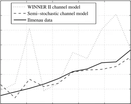
An example of the CIR produced by SSCM and the equivalent CIR for OFDM systems is shown in Figure 3.9.

3.4.4 Obtaining geographical information

To use the SSCM, precise geographical data is a prerequisite, however usually unavail-able. The open source database open street map (OSM) provides free information

(43)

about the accurate building shapes [1]. The coverage of OSM includes the majority of populated area in Europe. Figure 3.10 (a) shows a part of the city Munich. Since the purpose of OSM is map usage, there is only little of height information, which has to be obtained from other sources.

As a feature of most European cities, neighboring buildings generally have similar heights. Thus, a uniform height can be assigned to the buildings to achieve a good estimation. Figure 3.10 (b) is constructed from the OSM data with an uniform height information from estimation. Some previous works show that ray-tracing can still deliver good results with a 2.5D map with uniform height information [38].

(44)

(a)

(b)

Figure 3.10: (a) Building information of a part of Munich. Building edges are marked with solid lines. (b) Reconstructed 2.5 D geographical data using uniform building height

(45)

4 Feedback Strategies for Link level

Information

In cellular systems, to facilitate radio resource management, the downlink channel state information (CSI) is measured by the MS and it is send back to the BS via uplink transmission. The feedback operation must be done periodically, since the mobile radio channel is always changing. Therefore, to improve the uplink data throughput, the signaling overhead caused by this feedback information should be minimized. In LTE systems, a 4-bit channel quality indicator (CQI) is specified to carry the CSI [8]. The highly quantized CQI results in several problems. Firstly, in frequency selective channels, different subcarriers have a different frequency response. However, the LTE CQI feedback is not specified on subcarrier level, but on subband level. And each subband consists a number of subcarriers. Hence, the different CSI on different sub-carriers must be properly mapped into one single CQI. The mapping from CSI to CQI is discussed in Section 4.1. Secondly, after the CQI is transmitted from the MS, there is always a delay, before it is used in the BS to determine the resource alloca-tion. If this period is longer than the channel coherence time, the CQI used at the BS could be already outdated. As a result, the temporal variation of the channel should be compensated with channel prediction. The compensation of temporal variation is addressed in Section 4.3. Moreover, channel prediction schemes behave differently in systems with HARQ, which is explained in Section 4.4. In addition, the CQI has a strong relation to the resource allocation algorithm in multi-user systems. This issue is investigated in 4.5.

Parts of this chapter have been published in [64], [99], [102] and [100].

4.1 Information feedback in cellular networks

In LTE, depending on the periodicity of the CQI reporting modes, the feedback infor-mation is sent via the physical uplink control channel (PUCCH) or the physical uplink shared channel (PUSCH). And the down link data is transmitted via the PDSCH, where the modulation and coding schemes depend on the feedback information [5].

4.1.1 LTE resource structure and CQI basics

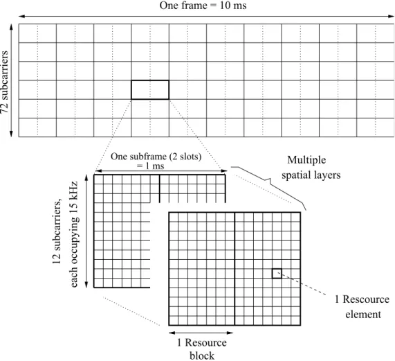
The LTE frame structure in physical downlink shared channel (PDSCH) is shown in Figure 4.1. As the smallest unit in the LTE transmission structure, the resource

(46)

ele-Figure 4.1: Resource structure of LTE

ment (RE) is defined as 1 subcarrier times 1 OFDMA symbol. A slot, which is made up by 7 OFDMA symbols with normal cyclic prefix or 6 OFDMA symbols with extended cyclic prefix, has a length of 0.5 ms in time domain. The basic unit for resource alloca-tion is the physical resource block (PRB), which consists of 12 consecutive subcarriers in 1 slot [8]. In spatial multiplexing mode, a few spatial layers can be transmitted at the same time. A frame of a duration of 10 ms consists of 10 subframes, and each subframe consists of 2 slots.

As a feature of OFDMA, a different modulation and coding scheme (MCS) can be applied to different PRB. Moreover, the MCS is adaptive to channel conditions, where the base stations can choose either higher data rate or better error protection, accord-ing to the channel quality [6]. To facilitate adaptive modulation and codaccord-ing (AMC), UEs must measure the channel quality and send the information to base stations. To reduce the signaling overhead, the channel quality information is compressed into a 4 bit CQI in LTE standards [8].

The CQI works as an index of the MCS. The correspondence between the CQI and the MCS is shown in Table 4.1. Smaller CQI values correspond to lower modulation orders

(47)

4.1 Information feedback in cellular networks

Figure 4.2: SINR to CQI mapping for SISO transmission CQI index Modulation Code rate × 1024 Efficiency [bit/s/Hz]

0 out of range 1 QPSK 78 0.1523 2 QPSK 120 0.2344 3 QPSK 193 0.3770 4 QPSK 308 0.6016 5 QPSK 449 0.8770 6 QPSK 602 1.1758 7 16QAM 378 1.4766 8 16QAM 490 1.9141 9 16QAM 616 2.4063 10 64QAM 466 2.7305 11 64QAM 567 3.3223 12 64QAM 666 3.9023 13 64QAM 772 4.5234 14 64QAM 873 5.1152 15 64QAM 948 5.5547

Table 4.1: The 4-bit CQI table in LTE [8]

and smaller code rates. Therefore, the data is better protected against distortion. And larger CQI values correspond to higher order modulation and higher code rates, such that higher data rate can be achieved. Accordingly, the CQI can be defined as

Definition 1. The CQI is the highest index in Table 4.1, whose MCS leads to a block error rate (BLER) not higher than 0.1 in the current channel condition.

Moreover, to further reduce the usage of uplink bandwidth, the feedback information is generated on subband level. A subband is defined as a group of consecutive PRBs. The CSI of all the PRBs within a subband is compressed into only one CQI message. Therefore, the CSI, namely, the SINR, of each PRB must be properly mapped into a single value. In fact, the SINR to CQI mapping consists of two steps, as illustrated in Figure 4.2. The measured SINRs are first compressed into a real valued effective SNR. The effective SNR is then mapped into an integer CQI.

(48)

−15 −10 −5 0 5 10 15 20 10−2 10−1 100 SNR [dB] BLER CQI 1 CQI 2 CQI 3 CQI 4 CQI 5 CQI 6 CQI 7 CQI 8 CQI 9 CQI 10 CQI 11 CQI 12 CQI 13 CQI 14 CQI 15

Figure 4.3: BLER for CQI 1-15 in AWGN channel

4.1.2 SINR to CQI mapping

To improve network capacity, the frequency reuse factor in LTE is 1. Therefore, strong co-channel interference (CCI) is to be expected. Consider a downlink system with S

cells, where an arbitrary UE i is served by the cell s. The Tx power is uniformly distributed among subcarriers and the OFDMA signals are perfectly synchronized. The frequency domain SINR of user i on subcarrier k is given as

γ(t, k) = |Hi,s(t,k)|2Gs(t,k)Us(t,k) Li,s(t,k) P j∈S\s |Hi,j(t,k)|2Gj(t,k)Uj(t,k) Li,j(t,k) +σ 2 w , (4.1)

whereU is the Tx power, Gis the antenna gain of the BS, Lis the pathloss, H is the normalized CFR for fast fading process,S is the set of cells andσ2

w is the noise power. Due to frequency selectivity, different PRBs generally have different SINRs. To find a proper value for the CQI, SINRs on different PRBs must first be mapped into an effective SNR. The BLER is the most popular criterion for the SINR to effective SNR mapping.

Since the CQI feedback is done on subband level, all the PRBs in the same subband would have the same MCS. With perfect channel knowledge, the CQI Q(t, κ) is the index of MCS for an arbitrary PRB κ in subbandb, as given in Table 4.1. The BLER of the transmission is jointly determined by the MCS and effective SNR of the wireless channel as Pe(Q(t, κ), γe(t, b)).

(49)

4.1 Information feedback in cellular networks 0 20 40 60 80 100 −20 −15 −10 −5 0 5 10 15 20 25 30 Time [ms] SINR or SNR [dB] SINR on 1st PRB SINR on 2nd PRB SINR on 3rd PRB SINR on 4th PRB Effective SNR

Figure 4.4: SINR to effective SNR mapping for 4 PRBs, using EESM

The BLER of transmission with different SINR in a frequency selective fading channel should match the BLER of transmission with the effective SNR in an AWGN channel. It can be written as:

Pe(Q(t, κ), γe(t, b)) =Pe(Q(t, κ), γ(t, k), κ∈ Ki, k ∈ Bi(b)), (4.2)

where Pe is the BLER, γe is the effective SNR, K is the set of PRBs, andBi(b) is the set of subcarriers in subband b. The BLER performance using the modulation and coding scheme specified in Table 4.1 in AWGN channel is shown in Figure 4.3.

One commonly used SINR to effective SNR mapping scheme is the exponential effective SINR mapping (EESM) [28]. Using EESM, the effective SNR can be written as

γe(t, b) = −βln   1 Nb X k∈Bi(b) exp −γ(t, k) β  , (4.3)

where Nb is the number of subcarriers in set Bi(b), the calibration parameter β needs to be empirically fine-tuned as a function of MCS and packet length. The fine-tuning can be done by minimizing the SINR compression error with extensive simulations [63]. Following the 3GPP specification of transmission blocks [6] and implementation of the Turbo decoder described in [82], the optimal values of β are summarized in

(50)

CQI 0 1 2 3 4 5 6 7

β n/a 4.40 4.07 4.22 3.87 4.57 4.68 5.85

CQI 8 9 10 11 12 13 14 15

β 3.77 3.97 3.71 3.06 3.20 3.04 2.41 1.88 Table 4.2: Optimal value forβ in LTE

CQI 0 1 2 3 4 5 6 7

SNR[dB] −∞ -6.59 -4.94 -2.90 -1.04 1.08 2.78 5.02

CQI 8 9 10 11 12 13 14 15

SNR[dB] 6.89 8.70 10.74 12.78 14.64 16.42 18.20 20.19 Table 4.3: Minimum effective SNR for CQI feedback

Table 4.2. An example of SINR to effective SNR mapping using EESM is given in Figure 4.4.

According to Definition 1, the effective SNR to CQI mapping function can be easily derived by applying a horizontal line for Pe = 0.1 in Figure 4.3. Each intersection point indicates the minimal SNR for the corresponding CQI, as shown in Table 4.3. Consequently, a step mapping function can be obtained, as illustrated in Figure 4.5.

4.1.3 Throughput and CQI feedback

The most important QoS metric in LTE is data throughput. Consider a single user case. Suppose perfect CSI is available and the MCS is always matched to the channel condition as described in Table 4.1. The probability of a successful transmission is

P0(Q(t, κ), γe(t, b)) = 1−Pe(Q(t, κ), γe(t, b)). (4.4)

Thus, the bandwidth efficiency of a certain PRB can be written as

E(t, κ) =η(Q(t, κ))P0(Q(t, κ), γe(t, b)), (4.5)

where η is the spectral efficiency as a function of the MCS, which can be found in Table 4.1. And the average throughput of this user is given by

F(t) = X κ∈K

B·E(t, κ), (4.6)

where B is the bandwidth of a PRB.

The relationship of bandwidth efficiency and effective SNR is shown in Figure 4.6. Since the MCS is directly associated with CQI, a noisy CQI feedback leads to an reduced throughput.