For Peer Review
Insights into Multiple/Single Lower Bound
Approximation for Extended Variational Inference
in Non-Gaussian Structured Data Modeling
Zhanyu Ma, Senior Member, IEEE,Jiyang Xie, Student Member, IEEE, Yuping Lai, Member, IEEE, Jalil Taghia,Member, IEEE, Jing-Hao Xue, and Jun Guo
Abstract—For most of non-Gaussian statistical models, the data being modeled represent strongly structured properties, such as scalar data with bounded support (e.g., beta distribution), vector data with unit length (e.g., Dirichlet distribution), and vector data with positive elements (e.g., generalized inverted Dirichlet distribution). In practical implementations of non-Gaussian statistical models, it is infeasible to find an analytically tractable solution to estimating the posterior distributions of the parameters. Variational inference (VI) is a widely used framework in Bayesian estimation. Recently, an improved frame-work, namely the extended variational inference (EVI), has been introduced and applied successfully to a number of non-Gaussian statistical models. EVI derives analytically tractable solutions, by introducing lower-bound approximations to the variational objective function. In this paper, we compare two approximation strategies, namely the multiple lower-bounds (MLB) approxima-tion and the single lower-bound (SLB) approximaapproxima-tion, which can be applied to carry out the EVI. For implementation, two differ-ent conditions, the weak and the strong conditions, are discussed. Convergence of the EVI depends on the selection of the lower-bound, regardless of the choice of weak or strong condition. We also discuss the convergence properties to clarify the differences between MLB and SLB. Extensive comparisons are made based on some EVI-based non-Gaussian statistical models. Theoretical analysis is conducted to demonstrate the differences between the weak and strong conditions. Experimental results based on real data show advantages of the SLB approximation over the MLB approximation.
Index Terms—Structured data, Beyesian estimation, non-Gaussian statistical models, extended variational inference, lower-bound approximation
I. INTRODUCTION
G
Aussian distribution is a ubiquitous probability distri-bution used in statistics, signal processing, and pattern recognition [1]. However, in reality data may be neither Gaussian nor safely assumed to be Gaussian [2]. In many real-life applications, the data are well-structured and, therefore, not Gaussian distributed [3]. For example, the image pixel values [4], the reviewer’s rating of an item in a recommenda-tion system [5], [6], and the DNA methylarecommenda-tion level data [7]Z. Ma, J. Xie, and J. Guo are with the Pattern Recognition and Intelligent System Lab., Beijing University of Posts and Telecommunications, Beijing, China.
Y. Lai is with the Department of Information Security, North China University of Technology, Beijing, China.
J. Taghia is with the Department of Information Technology, Division of Systems and Control, Uppsala University, Uppsala, Sweden.
J.-H. Xue is with the Department of Statistical Science, University College London, London, United Kingdom.
The corresponding author is Z. Ma. Email: [email protected]
are distributed in a range with bounded support. The diversity gain over theKG fading [8] and the periodogram coefficients
in speech enhancement [9] are semi-bounded (nonnegative). The spatial fading correlation [10] and the yeast gene ex-pressions [11] have directional characteristics for which data are assumed to be distributed on a unit hypersphere, i.e., satisfying l2 unit norm. In signal processing, the acoustic
noise with colored spectra [12] and the measurement noise in the state-space model [13] are heavy-tailed. In the stock market, the asymptotic behavior of the first-order autoregres-sive (AR) process is clearly non-Gaussian [14] and the un-derlying Bayesian copula model for the stock index series are similarly non-Gaussian [15]. Although the above mentioned data represent diverse characteristics, a common property is that these datanot onlyhave specific support ranges,but also have “non-bell” distribution shapes. The natural properties of a Gaussian distribution (the definition domain is unbounded and the distribution shape is symmetric) do not fit such data well. It has been found in recent studies that explicitly utilizing the non-Gaussian characteristics can significantly improve the practical performance on non-Gaussian structured data [2], [4], [7]–[9], [11]–[13], [16]. Hence, it is of particular importance and interest to make thorough studies of non-Gaussian data and non-Gaussian statistical models.
Bayesian analysis plays an essential role in parameter esti-mation of statistical models [17]–[22]. Unlike the convention-ally used maximum-likelihood (ML) estimation [23], Bayesian estimation assumes that the parameters are random variables with prior distributions, and derives the posterior distributions of the parameters by applying the Bayes theorem [24] through combining the prior distributions with the likelihood function obtained from the observed data [17], [25]. Estimation of the posterior distribution via Bayesian estimation has several advantages over the ML estimation. Firstly, it gives proba-bilistic description to the parameters, rather than simple point estimates yielded by the ML estimation. This makes Bayesian estimation more robust and reliable, by including the resulting uncertainty into the estimation [18]. Secondly, it can potential-ly prevent the overfitting problem, which is a main drawback of the ML estimation. This robustness against overfitting comes from marginalization, by integrating out uncertainties. Last but not the least, Bayesian estimation embodiesOccam’s razor[26], which allows a model to automatically regulate the model complexity. In the ML estimation, determination of the model complexity often requires cross validations, which can
4 5 6 7 8 9 10 11 12 13 14 15 16 17 18 19 20 21 22 23 24 25 26 27 28 29 30 31 32 33 34 35 36 37 38 39 40 41 42 43 44 45 46 47 48 49 50 51 52 53 54 55 56 57 58 59 60
For Peer Review
be non-optimal and computationally costly [17].Varitional inference (VI), among others, is a widely used strategy to infer the posterior distributions of the parameters in Bayesian analysis [17], [27]. In a fully Bayesian model where all variables are assigned with prior distributions, the task is to minimize the Kullback-Leibler (KL) divergence from the true posterior to the approximating posterior [17, Ch. 10]. In variational inference, the difficulty in minimizing the KL divergence of the true one from the approximating posteriors is cast alternatively as a less challenging task of maximizing a lower-bound defined on the marginal likelihood (model evidence). During optimization, the posterior distributions over all the variables are updated by iteratively updating one variable (or one group of variables) in turn, while keeping the other variables unchanged. VI has been successfully applied to many Gaussian models [1], [17]. However, for many non-Gaussian statistical models, maximizing the lower-bound still involves intractable moment computations, and consequently the resulting posteriors are not available in a closed-form solution. Examples of such models previously studied in the literature are: beta mixture model (BMM) [4], Dirichlet mix-ture model (DMM) [28], [29], generalized Dirichlet mixmix-ture model (GDMM) [30], inverted-Dirichlet Mixture Model (iD-MM) [31], [32], generalized inverted-Dirichlet mixture model (GiDMM) [33], von-Mises Fisher mixture model (VMM) [11], Watson mixture model (WMM) [34], and beta-Gamma non-negative matrix factorization (BG-NMF) [5]. Numerical meth-ods, e.g., Gibbs sampling and Markov chain Monte Carlo, are usually employed to sample from the posterior distribu-tion [27]. Numerical methods are generally computadistribu-tionally costly, and diagnosing their convergence can be difficult, in particular for data from a high-dimensional space [35].
Recently, an improved framework, namely the extended variational inference (EVI) [4], [5], [11], [28], [29], [36]–[38], has become popular in solving the above mentioned problem. Similar to the classic VI framework, EVI seeks an optimal approximation to the posterior distribution. The difference is that EVI relaxes the objective function (the evidence bound to the marginal likelihood) by constructing a lower-bound approximation to the objective function. Maximization of the EVI lower-bound, which uses the convexity or relative convexity [39] of the objective function, can yield analytically tractable solution so that the parameter estimation is facilitated. Although extra systematic bias has been introduced due to the lower-bound approximation, several works have demon-strated the advantages of EVI in Bayesian estimation of sta-tistical models [4], [5], [11], [29], [37]. In Bayesian estimation of BMM, Ma et al. [4] derived an analytically tractable solution which outperforms the numerical Gibbs sampling based method. As an extension of [4], Bayesian estimation of DMM via EVI has been proposed in [28] and [29], respec-tively. For directional data, von-Mises Fisher distribution is an important model in several applications. Analytically tractable solution to Bayesian estimation of VMM has been proposed by using EVI [11]. In Bayesian estimation of VMM, EVI was also applied in deriving analytically tractable solution [34]. For non-negative matrix factorization (NMF), EVI was also applied in deriving analytically tractable solutions for Poisson
process (discrete) NMF [40], Gamma process NMF in music recording [37], and beta-Gamma NMF for bounded support data [5].
Convergence is an important issue in parameter estima-tion. For VI-based methods, the objective function maximized during each iteration is convex or relatively convex [39] in terms of the target variable’s posterior distribution [17]. Hence, the convergence is theoretically guaranteed. In EVI, the introduced lower-bound approximation to the objective function can be obtained via either a single extension over the whole variable group or multiple extensions, one for a subset of the whole variable group. Based on this, two lower-bound approximation strategies are obtained: one is the single lower-bound (SLB) approximation [5], [11], [29], [37] and the other is the multiple lower-bounds (MLB) approximation [4], [28]. For EVI with the SLB approximation, convergence is also guaranteed because the VI objective function is replaced by a single lower-bound called the EVI lower-bound (i.e., the single lower-bound to the original objective function in VI). The EVI lower-bound is convex or relatively convex and tight to the VI objective function, and thus theoretically guaranteed to be maximized with each iteration. However, when applying EVI with the MLB approximation, the variable group is divided into different disjoint subsets and there exist different lower-bound approximations to the objective function. During each iteration, different lower-bounds, one for each variable subset, are maximized iteratively. Since the new objective function is not unique, convergence cannot be theoretically guaranteed.
In order to clarify the convergence property of the EVI framework, we will discuss and summarize the conditions required in the EVI implementation. The SLB and MLB ap-proximations will also be analyzed and compared qualitatively and quantitatively. It is worth to note that all the models we select and study in this paper (i.e., BMM, DMM, and GiDMM) are typical non-Gaussian statistical models which have both SLB and MLB derivations. Other non-Gaussian models, which do not have both representations, are not discussed in this paper.
II. VARIATIONALINFERENCE ANDEXTENDED
VARIATIONALINFERENCE
A. Variational Inference
In Bayesian estimation, a universal solution to the variation-al inference (VI) framework [41] is to approximate the pos-terior distribution by a product of several factor distributions and then update each factor distribution individually [17]. This method is the so-called factorized approximation (FA) which was developed from the mean field theory in physics [42]. With the FA method, the variational objective function that we want to maximize can be represented as
L= ! q(Z) lnp(X,Z) q(Z) dZ =EZ[lnp(X,Z)−lnq(Z)], (1)
whereXis the observed data, andZdenotes all the latent ran-dom variable and parameters. IfZcan be (approximately)
fac-5 6 7 8 9 10 11 12 13 14 15 16 17 18 19 20 21 22 23 24 25 26 27 28 29 30 31 32 33 34 35 36 37 38 39 40 41 42 43 44 45 46 47 48 49 50 51 52 53 54 55 56 57 58 59 60
For Peer Review
TABLE I
REQUIRED CONDITIONS FOREVI.
Auxiliary function Form of the Auxiliary Function Systematic Gap Strong condition p(X,Z)≥p"s(X,Z) E
Z\Zi[lnp"(X,Z)]!lnpi(Zi)† Gs>Gw
Weak condition EZ[lnp(X,Z)]≥EZ[lnp"w(X,Z)]
† “!” denotes that the two formulations at the LHS and RHS have the same mathematical form, up to a constant difference.
torized intoM disjoint groups asZ={Z1, . . . ,Zi, . . . ,ZM}
and we approximate the true posterior distributionp(Z|X)as p(Z|X)≈q(Z) =
M
#
i=1
qi(Zi), (2)
the optimal solution can be written as
lnq∗i(Zi) =EZ\
Zi[lnp(X,Z)] +const. (3)
The operator EZ\Zi means expectation with respect to all
the variables in Z except for Zi. If the optimal solution to
the posterior distribution of Zi, which is lnq∗i(Zi) in (3),
has the same logarithmical form as the prior distribution, the conjugate match between the prior and posterior distributions are satisfied. Then we have obtained an analytically tractable solution. However, this conjugate match is not satisfied in most of the practical problems [4], [5], [28], [29]. This is due to the fact that the optimal solution depends on the expectation computed with respect to the factor distribution [17]. B. Extended Variational Inference
In order to satisfy the conjugate match requirement, some approximations can be applied to get a nearly optimally analytically tractable solution. Braun et al. [38] considered the zeroth-order and first-order delta method for computation of moments to derive an alternative for the objective function to simplify the calculation. Blei et al. [36] proposed a correlated topic model (CTM) and used a first-order Taylor expansion to preserve a bound such that an intractable expectation was avoided. Similar ideas were also applied in [4], [11], [28], [29] for approximating the posterior distributions in BMM, DMM, and VMM, respectively. Using Jensen’s inequality has become commonplace in variational inference. In [37], the concavity of the function−x−1and the convexity of−logx
were studied and the Jensen’s inequality and the first-order Taylor expansion were applied to approximate the posterior distribution. Moreover, the EVI strategy was also applied in the low rank matrix approximation area [5], where the Taylor expansion and Jensen’s inequality were both applied for the purpose of deriving analytically tractable solutions.
All the aforementioned works utilized the following prop-erty. Given an auxiliary functionp"(X,Z)which satisfies
EZ[lnp(X,Z)]≥EZ[ln"p(X,Z)] for allX, (4)
the variational objective function (see [17], pp. 465 for more details) can be lower-bounded as
L=EZ[lnp(X,Z)]−EZ[lnq(Z)]
≥EZ[ln"p(X,Z)]−EZ[lnq(Z)] !L."
(5)
Then we can maximize the EVI lower-boundL, which is a" lower-bound to the original objective functionL. SinceL"is tight toLat least at one-point, maximizingL"would similarly maximizesL[4], [28], [29], [37]. The approximated optimal solution in this case is written as
ln"q∗
i(Zi) =EZ\Zi[lnp"(X,Z)] +const. (6)
This method is the so-called EVI framework [4], [5], [11], [28], [29], [36]–[38]. Although it introduces systematic gap when involving the lower-bound approximation, the EVI al-lows more flexibility when calculating intractable integrations in non-Gaussian statistical models and provides a convenient way to obtain an analytically tractable solution.
In addition, the proposed EVI framework, similar to the conventional VI framework, can also be applied to implicit distributions [43]. The implicit distributions are a family of probability models that the PDF is intractable, but there exists a way to sample from them and/or approximate expectations under them and calculate the gradients w.r.t. the model pa-rameters. In principle, the EVI framework can provide a more flexible approximation to the original lower bound for the purpose of providing the tools to handle the inference of the implicit distributions.
III. CONVERGENCE OFEVI
We first compare the weak and strong conditions quanti-tatively. Secondly, we intensively compare the performance of the MLB approximation-based methods with the SLB approximation-based methods. The selected models are typical and widely applied non-Gaussian statistical models.
A. Typical non-Gaussian Statistical Models • Beta mixture model (BMM)
Following the same notation in [4], we denote a BMM with observation datax= {x1, . . . , xN}and I mixture
components as f(x;π,u,v) = N # n=1 I $ i=1 πiBeta(xn;ui, vi), (7)
whereπi is the mixture weight for theith mixture
com-ponent withπi>0, %Ii=1πi= 1,u= [u1,· · ·, uI], and
v = [v1,· · ·, vI]. Beta(x;u, v) is the beta distribution,
which can be presented as
Beta(x;u, v) = Γ(u+v)
Γ(u)Γ(v)x
u−1(1−x)v−1, u, v >0,
(8) where x ∈ [0,1] and Γ(·) is the gamma function defined as Γ(z) = &0∞tz−1e−tdt. The beta mixture
4 5 6 7 8 9 10 11 12 13 14 15 16 17 18 19 20 21 22 23 24 25 26 27 28 29 30 31 32 33 34 35 36 37 38 39 40 41 42 43 44 45 46 47 48 49 50 51 52 53 54 55 56 57 58 59 60
For Peer Review
model has been widely applied in modeling non-Gaussiandistributed data with bounded support, such as image pixels, the ratings assigned to an item in collaborative fil-tering [6], and the epigenetic mark values in epigenome-wide-association studies [5], [44].
• Dirichlet mixture model (DMM)
If a K dimensional vectorx = [x1, . . . , xK]T contains
only positive values and the summation of all the K elements is smaller than one, the underlying distribution of x could be modeled by a Dirichlet distribution. The probability density function (PDF) of a Dirichlet distri-bution is [29] Dir(x;u) = Γ '%K+1 k=1 uk ( )K+1 k=1 Γ(uk) K+1# k=1 xuk−1 k , (9) where0< xk <1,xK+1= 1−%Kk=1xk,uk>0 and
u= [u1, . . . , uK+1]T is the parameter vector. The shape
of the Dirichlet distribution depends on the parameters. WithI mixture components, a DMM can be represented, given a set ofN i.i.d.observationsX= [x1, . . . ,xN], as
f(X;Π,U) = N # n=1 I $ i=1 πiDir(xn;ui), (10)
whereπi >0, %Ii=1πi = 1,Π = [π1, . . . ,πI]T is the
mixture weights andU= [u1, . . . ,uI]is the parameter
matrix. For modeling the data representing proportion-s, e.g., the weighting factors in a mixture model [17], and the topic model in document analysis [45], [46], the Dirichlet distribution and the related DMM have been extensively used.
• Generalized inverted-Dirichlet model (GiDMM)
Assume X = {x1,· · ·,xN} is a set of K-dimensional
observations, where each vectorxn is generated from a
GiDMM withI mixture components [33], [47]
f(X;Π,U,V) = N # n=1 I $ i=1 πiGiDir(xn;ui,vi), (11)
where Π = [π1, . . . ,πI]T is the mixture weight vector
subject to the constraints πi > 0 and %Ii=1πi= 1,
U = [u1,· · ·,uI] and V = [v1,· · ·,vI] are the set
of parameters. GiDir(x;u,v) is a generalized inverted-Dirichlet distribution with its own positive parameter vectorsu= [u1,· · ·, uK]T andv= [v1,· · ·, vK]T as GiDir(x;u,v) = K # k=1 Γ(uk+vk) Γ(uk)Γ(vk) · x uk−1 k (1 +%Kk=1xk) γk, (12) where Γ(·) represents the Gamma function,γk = uk+
vk−vk+1 fork= 1,· · ·, K andvK+1= 0.
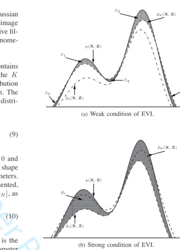
For positive data which are naturally generated by several real life applications, the GiDMM, among others, has been utilized for the purpose of clustering and classification of such data [33], [48]. p(X,Z) ! pw(X,Z) ! ps(X,Z) S1 S2 S3 S4 S5
(a)Weak condition of EVI.
p(X,Z) ! pw(X,Z) ! ps(X,Z) Gs
(b)Strong condition of EVI.
Fig. 1. Comparisons of the weak and strong conditions of EVI for a multi-modal distribution. The systematic gap introduced by the weak
condition can be calculated asGw= (S1+S2)−(S3+S4+S5). For
either the strong or weak condition, the auxiliary function is chosen to minimize the gap as much as possible. Generally speaking, the
systematic gapGwis smaller thanGs.
B. Weak Condition and Strong Condition
As mentioned in Sec. II-B, finding an auxiliary function "
p(X,Z)is an essential yet difficult part in EVI implementa-tion. Generally speaking, this auxiliary function should satisfy the relation presented in (4) or it should satisfy
p(X,Z)≥p"(X,Z), for allXand Z. (13) It is straightforward to show that an auxiliary function which satisfies (13) should also satisfy (4). Hence, the condition in (4) is named as the weak condition and the one in (13) is referred to as thestrong condition. When using an auxiliary function to lower-bound the original objective function, the EVI will introduce a systematic gap. Generally speaking, the gap1 incurred by applying the weak condition is relatively
smaller than that introduced by using the strong condition. Figure 1 illustrates the different gaps introduced by the weak and strong conditions, respectively.
It is worthwhile to note that the auxiliary functionp"(X,Z)
is not necessary to be a normalized probability density function (PDF)2. This will not affect the final solution since either
VI or EVI will re-normalize the obtained optimal posterior 1We calculate the gap via sampling methods.
2Actually, an auxiliary function that satisfies the strong condition cannot
be a normalized PDF, asp(X,Z)itself is a normalized PDF.
5 6 7 8 9 10 11 12 13 14 15 16 17 18 19 20 21 22 23 24 25 26 27 28 29 30 31 32 33 34 35 36 37 38 39 40 41 42 43 44 45 46 47 48 49 50 51 52 53 54 55 56 57 58 59 60
For Peer Review
distribution in the end. For example, the optimal solution to" q∗
i(Zi)can be obtained by normalizing the RHS of (6) as
" qi∗(Zi) = exp (lnq" ∗ i(Zi)) & exp (ln"q∗ i(Zi))dZi = exp'EZ\Zi[lnp"(X,Z)] ( & exp'EZ\Zi[lnp"(X,Z)] ( dZi , (14)
where the constant part that does not containZi is cancelled
at the numerator and the denominator. More examples can be referred to [17, Chap. 10].
In practice, in addition to the above mentioned weak or strong condition, an auxiliary function should also have a specific mathematical form so that the optimal solution in (6) has the same logarithmic form as the prior distribution such that the conjugate match between the prior and the posterior is satisfied. This is another required condition for choosing the auxiliary function. Table I lists the required conditions when implementing EVI. In summary, in order to apply the EVI to derive an analytically tractable solution to the Bayseisn estimation of non-Gaussian statistical models, an auxiliary function should 1) satisfy either the weak or strong condition and 2) have the same mathematical form as the prior distribution (up to a constant difference).
1) Discussion:Generally speaking, it is usually not feasible to find an auxiliary function that satisfies the strong condition, except that the original functionp(X,Z)is globally concave in terms of Z 3. Unlike the case of the strong condition, it is relatively easy to find an auxiliary function to fulfill the weak condition, as the original function p(X,Z) might be partially concave with respect to part of Z [5], [29]. For example [29], the multivariate log-inverse-beta (MLIB) function in the Dirichlet distribution is notglobally concave in terms of all of its variables. It is only relatively concavew.r.t. one of its variables when fixing the rest. Iteratively taking this property, an auxiliary function that satisfies the weak condition (with a proper expectation form) and the requirement of the mathematical form can be found so that an analytically tractable solution is derived. In practice, an auxiliary function that satisfies either the strong or weak condition is difficult to design/obtain. One way of obtaining an appropriate auxiliary function is to consider the Jensen’s inequality or the Taylor expansion, when combining with the convexity or relative convexity of the original function [2], [5].
In general, the weak condition yields smaller systematic gap in terms of approximation accuracy. Hence, if one can find an auxiliary function that satisfies the weak condition, there is no need to find another auxiliary function for the strong condition. 2) Comparisons of Weak and Strong Conditions: Since Dirichlet distribution is a multivariate case of beta distribution, the EVI-based Bayesian BMM that constructs an auxiliary function with the weak condition can be obtained based on the DMM work in [29] by simply setting the dimension to
2. The EVI-based Bayesian BMM proposed in [4] utilized the strong condition to choose the auxiliary function. Based 3According to our experience, for (most of) the non-Gaussian statistical
models, the original function is not globally concave.
on two different solutions for Bayesian estimation of BMM, we demonstrate the differences between the strong and weak conditions.
We consider the observationxnand the unobserved
indica-tor vecindica-torznas thecompletedata. The conditional distribution
of X = {x1, . . . , xN} and Z = {z1, . . . ,zN} given the
parameters{U,V,Π} is f(X,Z|U,V,Π) =f(X|U,V,Z)f(Z|Π) = N # n=1 I # i=1 [πiBeta(xn|ui, vi)] zni. (15)
The ultimate goal is to estimate the posterior distributions of ui,vi, andzni, respectively.
In order to derive an analytically tractable solution to the posterior distributions, the most challenging part with the EVI framework is to calculate the expectation of the bivariate log-inverse-beta (LIB) function
Eui,vi[LIB(ui, vi)] =Eui,vi * Γ(ui+vi) Γ(ui)Γ(vi) + . (16)
• EVI-based Bayesian BMM with Weak Condition [29] In the Bayesian BMM with SLB approximation 4, the
new objective function that we are maximizing is EZ[lnp"w(X,Z)] =L"SLB = lnΓ(ui+vi) Γ(ui)Γ(vi) +ui[ψ(ui+vi)−ψ(ui)] (E[lnui]−lnui) +vi[ψ(ui+vi)−ψ(vi)] (E[lnvi]−lnvi), (17)
where x is the expected value of x and ψ(x) is the digamma function defined as ψ(x) = ∂ln∂Γx(x). This lower-bound satisfies the weak condition such that EZ[lnp(X,Z)] ≥ EZ[lnp"w(X,Z)]. Moreover, this
lower-bound is identical for all the variablesui,vi, and
zni
• EVI-based Bayesian BMM with Strong Condition [4] In the case of the strong condition, an auxiliary function "
ps(X,Z) is required. In [4], three different auxiliary
functions were derived for the variablesui,vi, andzni,
respectively. To specify, forui, the auxiliary function is
" psui(X,Z) = ln Γ(ui+vi) Γ(ui)Γ(vi) +ui[ψ(ui+vi)−ψ(ui)] (lnui−lnui) +vi[ψ(ui+vi)−ψ(vi)] (lnvi−lnvi) +uiviψ ′ (ui+vi)(lnui−lnui), (18) 4A Bayesian BMM with SLB approximation can be derived from the
Bayesian DMM with SLB approximation [29] by setting the dimension of the Dirichlet variable to two.
4 5 6 7 8 9 10 11 12 13 14 15 16 17 18 19 20 21 22 23 24 25 26 27 28 29 30 31 32 33 34 35 36 37 38 39 40 41 42 43 44 45 46 47 48 49 50 51 52 53 54 55 56 57 58 59 60
For Peer Review
whereψ′(x) = ∂ψ∂(x)x . Hence, when consideringuias thevariable, the objective function that is maximized is [4] " LMLBui =EZ,p"sui(X,Z) -= lnΓ(ui+vi) Γ(ui)Γ(vi) +ui[ψ(ui+vi)−ψ(ui)] (E[lnui]−lnui) +vi[ψ(ui+vi)−ψ(vi)] (E[lnvi]−lnvi) +ui·vi·ψ ′ (ui+vi)(E[lnui]−lnui) +const. (19) Similarly, due to the symmetry ofuiandvi, the objective
function, when treatingvi as the variable, is [4]
" LMLBvi = lnΓ(ui+vi) Γ(ui)Γ(vi) +ui[ψ(ui+vi)−ψ(ui)] (E[lnui]−lnui) +vi[ψ(ui+vi)−ψ(vi)] (E[lnvi]−lnvi) +ui·vi·ψ ′ (ui+vi)(E[lnvi]−lnvi) +const. (20) When taking zni as the only variable, the auxiliary
function that proposed in [4] is " pszni(X,Z) = lnΓ(ui+vi) Γ(ui)Γ(vi) +ui[ψ(ui+vi)−ψ(ui)] (lnui−lnui) +vi[ψ(ui+vi)−ψ(vi)] (lnvi−lnvi) + 0.5·u2 i . ψ′(ui+vi)−ψ ′ (ui) / (lnui−lnui)2 + 0.5·v2i . ψ′(ui+vi)−ψ ′ (vi) / (lnvi−lnvi)2 +ui·vi·ψ ′ (ui+vi)(lnui−lnui)(lnvi−lnvi). (21) Correspondingly, the objective function for updating the posterior distribution ofzni can be written as
" LMLBzni =EZ , " pszni(X,Z) -= ln Γ(ui+vi) Γ(ui)Γ(vi) +ui[ψ(ui+vi)−ψ(ui)] (E[lnui]−lnui) +vi[ψ(ui+vi)−ψ(vi)] (E[lnvi]−lnvi) + 0.5·u2 i . ψ′(ui+vi)−ψ ′ (ui) / E,(lnui−lnui)2 -+ 0.5·v2i . ψ′(ui+vi)−ψ ′ (vi) / E,(lnvi−lnvi)2 -+ui·vi·ψ ′ (ui+vi)(E[lnui]−lnui)(E[lnvi]−lnvi).
It has been analyzed in Sec. III-B that both the strong condition and the weak condition incur systematic gaps. We now quan-titatively compare the gaps. It is worth to note that the EVI-based Bayesian BMM with the strong condition is also a MLB approximation. In principle, there exist four combinations, which are “strong condition+SLB”, “weak condition+SLB”, “strong condition+MLB”, and “weak condition+MLB”. We
focus only on the comparisons of weak and strong conditions in this section. The comparisons of the SLB approximation with the MLB approximation will be presented in the next section.
When takinguias the variable, the difference between the
objective functions obtained via weak and strong conditions, respectively, can be calculated as
∆L"SLB vs. MLBui =L"SLB−L"MLBui
=−u¯iv¯iψ′(¯ui+ ¯vi)(E[lnui]−ln ¯ui)
≥0,
(22) where we used the fact thatψ′(x)>0 and lnx is a convex function with respect tox. Forvi, it is straightforward to show
that the difference is also positive by using the symmetric properties.
When comparingL"SLB withL"MLBzni, the difference is ∆L"SLB vs. MLBzni =L"SLB−L"MLBzni =−00.5·u2i . ψ′(ui+vi)−ψ ′ (ui) / E,(lnui−lnui)2 -+ 0.5·v2i . ψ′(ui+vi)−ψ ′ (vi) / E,(lnvi−lnvi)2 -+ui·vi·ψ ′ (ui+vi)(E[lnui]−lnui)(E[lnvi]−lnvi) 1 .
It can be proved that the difference∆L"SLB vs. MLBzni is also
greater than or equal to0. More details for this proof can be found in Appendix A.
The aforementioned three positive differences indicate that the new objective function with the weak condition [29] is tighter (i.e., closer to the original objective function) than that with the strong condition [4]. Thus, for the EVI-based Bayesian BMM, the systematic gap incurred by the weak condition is smaller than that incurred by the strong condition. This makes the weak condition more favorable in practice [5], [11], [29], [37]. Similar analysis can be applied to the Bayesian DMM with MLB [28] and the Bayesian DMM with SLB [29], as Dirichlet distribution is a multivariate extension of beta distribution.
C. SLB Approximation and MLB Approximation
If we can find an auxiliary functionp"(X,Z)that contains all the variables Z and satisfies the aforementioned required conditions, the convergence of EVI is naturally guaranteed as this new objective function is convex or relatively convex in terms ofqi(Zi)[17]. Since only one lower-bound
approxima-tion is applied to the original objective funcapproxima-tion, this approach is referred to as the single lower-bound (SLB) approximation and has been applied in,e.g., [5], [11], [29].
When dividing Z into M disjoint groups as Z =
{Z1, . . . ,Zi, . . . ,ZM}, there might exist several auxiliary
5 6 7 8 9 10 11 12 13 14 15 16 17 18 19 20 21 22 23 24 25 26 27 28 29 30 31 32 33 34 35 36 37 38 39 40 41 42 43 44 45 46 47 48 49 50 51 52 53 54 55 56 57 58 59 60
For Peer Review
TABLE II
SLBANDMLBAPPROXIMATION COMPARISONS WITH DIFFERENT NON-GAUSSIAN STATISTICAL MODELS.
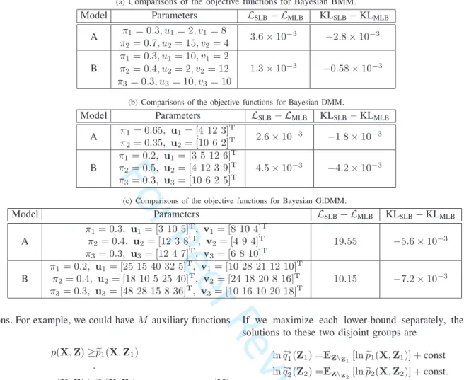
(a)Comparisons of the objective functions for Bayesian BMM.
Model Parameters LSLB−LMLB KLSLB−KLMLB A π1= 0.3, u1= 2, v1= 8 3.6×10⁻³ −2.8×10⁻³ π2= 0.7, u2= 15, v2= 4 B π1= 0.3, u1= 10, v1= 2 1.3×10⁻³ −0.58×10⁻³ π2= 0.4, u2= 2, v2= 12 π3= 0.3, u3= 10, v3= 10
(b) Comparisons of the objective functions for Bayesian DMM.
Model Parameters LSLB−LMLB KLSLB−KLMLB A π1= 0.65, u1= [4 12 3] T π2= 0.35, u2= [10 6 2]T 2.6×10 −3 −1.8×10⁻³ B π1= 0.2, u1= [3 5 12 6]T π2= 0.5, u2= [4 12 3 9]T π3= 0.3, u3= [10 6 2 5]T 4.5×10⁻³ −4.2×10⁻³
(c) Comparisons of the objective functions for Bayesian GiDMM.
Model Parameters LSLB−LMLB KLSLB−KLMLB A π1= 0.3, u1= [3 10 5]T, v1= [8 10 4]T π2= 0.4, u2= [12 3 8]T, v2= [4 9 4]T π3= 0.3, u3= [12 4 7]T, v3= [6 8 10]T 19.55 −5.6×10⁻³ B π1= 0.2, u1= [25 15 40 32 5]T, v1= [10 28 21 12 10]T π2= 0.4, u2= [18 10 5 25 40]T, v2= [24 18 20 8 16]T π3= 0.3, u3= [48 28 15 8 36]T, v3= [10 16 10 20 18]T 10.15 −7.2×10⁻³
functions. For example, we could haveM auxiliary functions as p(X,Z)≥p"1(X,Z1) · p(X,Z)≥p"i(X,Zi) · p(X,Z)≥p"M(X,ZM). (23)
This approach is referred to as the multiple lower-bound (ML-B) approximation. As each of the above mentioned auxiliary functions satisfies the required conditions in Sec. III-B, the optimal solution in (6) is
ln"q∗
i(Zi) =EZ[ln"pi(X,Zi)] +const= lnp"i(X,Zi) +const.
(24) In this case, the new objective function that is maximized during each iteration isnot unique. Hence,there is no globally objective function that is maximized during each iteration. Thus, the convergence cannot be theoretically guaranteed. This approach has been applied in [4] and [28]. Although con-vergence is not theoretically guaranteed, it can be monitored empirically.
Let us study a simple case with two disjoint groups in the MLB approximation. Assuming that Z = {Z1,Z2} and we
have two auxiliary functionsp"1(X,Z1)andp"2(X,Z2)forZ1
andZ2, respectively. As mentioned above, two different
lower-bounds are obtained as "
L1=EZ[lnp"1(X,Z1)−lnq(Z)]
"
L2=EZ[lnp"2(X,Z2)−lnq(Z)].
(25)
If we maximize each lower-bound separately, the optimal solutions to these two disjoint groups are
lnq"∗
1(Z1) =EZ\Z1[lnp"1(X,Z1)] +const (26a) lnq"∗
2(Z2) =EZ\Z2[lnp"2(X,Z2)] +const. (26b) With these solutions, it appears what we are maximizing is just two times of the original lower-bound as
2×L≥L"1+L"2 (27a) =EZ[ln"p1(X,Z1)]−EZ[lnq(Z)] (27b) +EZ[ln"p2(X,Z2)]−EZ[lnq(Z)]. (27c)
When performing the update strategy (26a), we get (27b) to be maximized. It is due to the fact that the optimal solution lnq"∗
1(Z1) maximizes L"1. This maximization makes
the distribution ofZ1 to be less uncertain. As−EZ[lnq(Z)]
in (27c) is the differential entropy ofZ, (27c) is decreasing while (27b) is maximizing. It is hard to evaluate if (27b) changes more than (27c) or not. Thus, the overall lower-bound, i.e., L21+L22 in (27a), might decrease during some
iterations. On the one hand, as the lower-bound (i.e.,L"1+L"2)
to the original objective function cannot be guaranteed to be maximized all the time, this strategy may not promise convergence. On the other hand, if the change in (27b) is larger than that in (27c), the convergence is still guaranteed. There is no general judgement for the convergence. It should be studied case by case. Similar arguments can be applied to the case with more than two auxiliary functions. Thus, the convergence of MLB approximation is unguaranteed. In summary, SLB approximation can theoretically guarantee the
4 5 6 7 8 9 10 11 12 13 14 15 16 17 18 19 20 21 22 23 24 25 26 27 28 29 30 31 32 33 34 35 36 37 38 39 40 41 42 43 44 45 46 47 48 49 50 51 52 53 54 55 56 57 58 59 60
For Peer Review
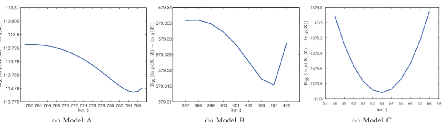
762 764 766 768 770 772 774 776 778 780 782 784 786 113.775 113.78 113.785 113.79 113.795 113.8 113.805 Iter.♯ EZ [l n p ( X , Z ) − ln q ( Z )] (a)Model A 397 398 399 400 401 402 403 404 405 579.31 579.315 579.32 579.325 579.33 579.335 Iter.♯ EZ [ln p ( X , Z ) − ln q ( Z )] (b)Model B 57 58 59 60 61 62 63 64 65 66 67 68 69 -1876 -1875.8 -1875.6 -1875.4 -1875.2 -1875 Iter.♯ EZ [ln p ( X , Z ) − ln q ( Z )] (c)Model CFig. 3. Observations of decreasing values of the objective function during iterations. In principle, objective function should always increase (at least not decrease). This non-convergence fact indicates that the MLB approximation-based method may not promise convergence. Model
A is a BMM with parameter π1 = 0.3,π2 = 0.7,u1 = [2 8]T,u2 = [15 4]T, model B is a three-dimensional DMM with parameter
π1 = 0.35,π2 = 0.65,u1 = [4 12 3]T,u2 = [10 6 2]T, and model C is a three-dimensional GiDMM with parameterπ1 = 0.3,π2 =
0.4,π3= 0.3,u1 = [3 10 5] T , v1= [8 10 4] T , u2= [12 3 8] T , v2 = [4 9 4] T , u3= [12 4 7] T , v3= [6 8 10] T .400samples were
generated from each model.
( ) Z E ⎡⎣lnpX, Z⎤⎦ ( ) Z E ⎡⎣lnp% X, Z⎤⎦ ( ) Z 1 1 E ⎡⎣lnp% X, Z ⎤⎦ ( ) Z 2 2 E ⎡⎣lnp% X, Z ⎤⎦
Fig. 2. Qualitative comparisons of SLB and MLB. For MLB, two
different lower-bounds are introduced for Z1 and Z2, respectively
(the blue lines). For SLB, there is only one lower-bound (the green line). The original objective function is marked with red solid line. It can be observed that the new objective function that needs to be maximized is not unique in the MLB case. Hence, the convergence is not guaranteed. A new single objective function is employed and maximized in the SLB case. Therefore, the convergence is theoretically guaranteed.
convergence while MLB approximation, in general, cannot promise convergence.5
1) Comparisons of MLB and SLB Approximations: In the previous section, we analyzed and compared the weak and strong conditions for the EVI framework. Another important issue in EVI implementation is to distinguish the MLB and SLB approximations, as the latter can guarantee convergence but the former may not. To this end, we compare the MLB based algorithm with the SLB approximation-based algorithm in this section.
• Observations of Oscillation
As discussed in Sec. III-C, the convergence of the MLB method is not guaranteed. We ran the ML-B approximation-based ML-Bayesian ML-BMM algorithm [4], Bayesian DMM algorithm [28], and Bayesian GiDM-M [48], respectively, and monitored the value of the objective function during each iteration. It was observed 5In practice (e.g., [4], [28]), the EVI-based algorithm may also converge
with MLB approximation. However, it is empirical result without proof.
that, for some rounds of simulations 6, the objective
function was oscillating during some iterations. This phenomenon was observed for several times, for BMM, DMM, and GiDMM. Figure 3 illustrates the decreasing objective function values and the corresponding itera-tions. For the SLB approximation-based Bayesian BMM and Bayesian DMM [29], the monitored objective func-tion was always increasing until convergence. The obser-vations of oscillation demonstrate that the convergence with MLB approximation cannot be guaranteed. • Comparisons of Estimation Accuracy
In this section, we compare the MLB approximation with the SLB approximation quantitatively. With a known BM-M or DBM-MBM-M or GiDBM-MBM-M,2,000samples were generated, respectively. The above-mentioned Bayesian estimation algorithms were applied to estimate the posterior distribu-tions, respectively. We calculated the original variational objective function in (1) to examine which approximation is better. With the obtained posterior distributionq∗(Z),
the original variational objective function is calculated numerically by sampling methods. Hence,we got two different values, LSLB and LMLB, from the SLB
ap-proximation and the MLB apap-proximation, respectively. Larger value means closer lower-bound approximation. In addition to this, we also measure the estimation accuracy by the KL divergence of the estimated PDF from the true one as KL(p(X|Θ)∥p(X|Θ2)), where Θ
is the true parameter vector andΘ2 is the estimated one. Similarly, we numerically calculated KLSLB and KLMLB
from the SLB and MLB approximations7, respectively.
The smaller the KL divergence is, the more accurate the estimation is.
For Bayesian BMM, comparisons are presented in Ta-ble II(a), Figure 4(a) and 4(d). The comparisons of the Bayesian DMM via SLB [29] and MLB [28] approxima-tions are illustrated in Table II(b), Figure 4(b) and 4(e). For GiDMM, the comparisons of Bayesian GiDMM via SLB (algorithm presented in Appendix B) and MLB [48] 6Here, one simulation round means that we ran the estimation algorithm
until it stops according to some criterion.
7For the MLB approximation, we only take those simulation rounds that
always converge into consideration.
5 6 7 8 9 10 11 12 13 14 15 16 17 18 19 20 21 22 23 24 25 26 27 28 29 30 31 32 33 34 35 36 37 38 39 40 41 42 43 44 45 46 47 48 49 50 51 52 53 54 55 56 57 58 59 60
For Peer Review
0.27 0.28 0.29 0.3 0.31 0.32 0.33 0.34 0.35 0.36 SLB MLB(a)Bayesian BMM: model A
1.5 1.55 1.6 1.65 1.7 SLB MLB (b) Bayesian DMM: model A -9400 -9350 -9300 -9250 -9200 -9150 -9100 -9050 SLB MLB
(c)Bayesian GiDMM: model A
0.025 0.03 0.035 0.04 0.045 0.05 0.055 0.06 0.065 SLB MLB (d)Bayesian BMM: model B 2.6 2.65 2.7 2.75 2.8 2.85 2.9 2.95 3 SLB MLB
(e)Bayesian DMM: model B
-1.265 -1.26 -1.255 -1.25 -1.245 -1.24 -1.235 104 SLB MLB ×
(f)Bayesian GiDMM: model B
Fig. 4. Comparisons of the original objective functions for Bayesian BMM, Bayesian DMM, and Bayesian GiDMM (with SLB and MLB,
respectively). For each sub-figure,20 rounds of simulations were conducted. In each boxplot, mark is the median, the box edges are the
25th
and75th
percentiles. The outliers are marked individually. Model settings are the same as Table II.
approximations are shown in Table II(c), Figure 4(c) and 4(f). All the simulations were run 20 rounds and the mean values are reported.
It can be observed that, for Bayesian BMM, Bayesian DMM and Bayesian GiDMM, the SLB approximation yields higher objective function value than the MLB approximation, respectively. Meanwhile, the KL diver-gences obtained by the SLB approximation are all smaller than those obtained by the MLB. The results suggest that the SLB approximation is superior to the MLB approximation.
IV. EXPERIMENTALRESULTS ANDDISCUSSIONS
In this section, we compare the SLB-based GiDMM with the MLB-based GiDMM using the tasks of text categorization, object detection, and image categorization.
We apply several statistical models to describe the under-lying distribution of the structured features extracted from text and images. It is worth noting that the main motivation of the real data evaluation is to evaluate and analyze the multiple/single lower bound approximations for non-Gaussian mixture models. Hence, we do not involve other non-mixture model-based methods for comparisons.
2) Text Categorization: With the development of internet, the amount of the text documents has been dramatically increased. If the text documents are organized and processed manually, it not only will consume a great deal of manpower, but also is hard to conduct efficient analysis [49], [50]. Hence, there exists urgent need to develop a technique which can organize the documents efficiently. In order to meet the re-quirements and challenges, automatic text categorization [50]–
[52], which is a key technique for processing and organizing vast amount of text data, has been widely applied. It has very realistic significance for efficient management and effective utilization of information and has gradually become an im-portant research direction in the domain of data mining [47]. Recently, different statistical model-based approaches have been proposed and utilized to carry out the text categorization task [30], [51]–[55].
In this paper, we report the experimental results by using the Bayesian GiDMM as a classifier for the task of text categorization on the dataset gathered from the top10largest categories of the “ModApte” split of the Reuters-215788. This
dataset is composed of9990news stories which were grouped into10categorizations. Each categorization is randomly split into two halves, one half for training and the other half for test. Following the work in [56], the Porter’s stemming [57] is used to reduce the words to their base forms. In this pre-processing stage, the words that occur less than3 times or are shorter than 2 in length are eliminated. Eventually, each document was represented by a 10-dimensional vector which contains only positive elements. Based on the aforementioned pre-processing, we trained a statistical model (Bayesian GiDMM with SLB approximation, denoted as “Bayesian GiDMMSLB”.
Detailed algorithm is presented in Appendix B) for each categorization and calculate the likelihood for the test vectors. A test document is considered correctly categorized if its corresponding model yields the highest likelihood. For com-parison, we have also applied four other approaches for catego-rizing text documents: the Bayesian GiDMM using the MLB
8http://kdd.ics.uci.edu/databases/reuters21578/ 4 5 6 7 8 9 10 11 12 13 14 15 16 17 18 19 20 21 22 23 24 25 26 27 28 29 30 31 32 33 34 35 36 37 38 39 40 41 42 43 44 45 46 47 48 49 50 51 52 53 54 55 56 57 58 59 60
For Peer Review
TABLE III
TEXT CATEGORIZATION ACCURACIES OBTAINED BY DIFFERENT METHODS.
Method Bayesian GiDMMSLB Bayesian GiDMMMLB Bayesian iDMMSLB Bayesian iDMMMLB Bayesian GMM
Accuracy (in%) 86.89 86.45 86.02 85.82 80.63
Runtime (in s)† 5.33 11.71 8.20 13.56 12.41
† On a ThinkCentre!computer with Intel!CoreTMi5−4590CPU4G.
approximation (denoted as “Bayesian GiDMMMLB” [48].),
the iDMM using the SLB and MLB approximation (which we refer to as “Bayesian iDMMSLB” [58] and “Bayesian
iDMMMLB” [59], respectively), and the Bayesian Gaussian
mixture model (Bayesian GMM) [17]. The main motivation is to validate the approaches of text categorization by considering comparable statistical model-based methods. Table III shows the categorization accuracies. It can be observed that the best performance is obtained by “Bayesian GiDMMSLB”, in
terms of the categorization accuracy rate (i.e.,86.89%), which demonstrates the advantage of using the SLB approximation over using the MLB approximation, for the non-Gaussian statistical model-based text categorization task. The reported values are the means of10times evaluations. In each evalua-tion, the aforementioned procedures are repeated.
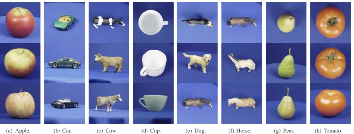
3) Object Detection: Object detection refers to the task of distinguishing a specific object (e.g., car, face) from other objects in an image, which is an essential task in computer vision. It has been a topic of extensive studies in the past decades. Object detection has various applications, such as robotics [60], medical image analysis [61], surveillance and human computer interaction [62]. Although humans usually perform well in object detection, it is much difficult to obtain similar performance for the machines, which is mainly due to the changes in illumination conditions, orientations, positions and scales. The aforementioned factors can dramatically affect the appearance of a given object. Recently, a great deal of re-search efforts have devoted to overcome such difficulties [33], [63]–[65]. These researches can be divided into two main categories. The first one has been devoted to the development of excellent global or local visual image descriptors [66]. The second one has been focusing on the development of powerful and robust classifiers [67].
As with the majority of computer vision tasks, a key step for accurate object detection is to extract good descriptors to represent these target objects. Recently, researchers have proposed many global and local visual descriptors, such as the Histogram of Oriented Gradient (HOG) descriptor [68], which is originally developed for detecting pedestrian in gray-scale images. Here, we use the rectangular HOG (denoted as RHOG) descriptor [69], which generates positive feature vectors. Moreover, it is found to be efficient and convenient for our object detection task. Experiments were conducted by considering seven windows for the RHOG descriptor, such that each image can be represented by a 441-dimensional feature vector. We use the publicly available ETH-80 dataset [70]. This dataset consists of 3280 images, which are categorized into eight object classes. Each class contains10unique objects and41views (i.e.,410images for each class). Example images from this dataset are shown in Figure 5. During the evaluation, we trained one detector for each class. For a given class, we take all the images from this class as the positive set and the
images in the negative set for this class were taken from the other seven remaining classes, where each class contributes
1/7 (approx. 58 images from each of the seven classes) to the negative examples. The detector was trained on half of the positive set and half of the negative set, where these two sets were randomly split into two equal parts, respectively. The remaining half of the positive and negative sets were used as the test set.
With the above training/test set selection, our methodology for object detection can be summarized as follows. First, RHOG descriptors were extracted from each image. By doing this, the description of each image was represented as a posi-tive vector. Second, each vector is assumed generated from a mixture of generalized inverted-Dirichlet distributions and we apply the proposed Bayesian GiDMMSLBas a classifier to
de-tect objects by assigning the test image to the group which has the highest posterior probability according to Bayes’ decision rule. Similar to the text categorization task in Sec. IV-2, we also train classifiers based on Bayesian GiDMMMLB, Bayesian
iDMMSLB, Bayesian iDMMMLB, and Bayesian GMM,
respec-tively. We report on the accuracies of the aforementioned five classifiers in Table IV. As can be observed from this table, the Bayesian GiDMMSLB achieves the best detection
rates, compared to the other referred methods. Similar to the task of text categorization, it is also observed that the SLB approximation is superior to the MLB approximation for both Bayesian GiDMM and Bayesian iDMM in the object detection task. We conducted10 rounds of simulations and the mean values are reported.
4) Image Categorization: With the development and broad applications of digital information acquiring techniques, the number of digital images has grown enormously. Image cat-egorization task is developed to meet the requirements of many important applications, such as image retrieval [71], content-based images recommendation [72], and automatic image understanding [73]. Recently, image categorization has emerged as an attractive area in computer vision [66], [74], [75]. A key step for accurate images categorization is to extract robust and efficient image descriptors to represent these images. Here, we use the RHOG descriptor [69] again by considering eight windows for the RHOG descriptor such that each image in the dataset was then represented by a 576 -dimensional feature vector.
The evaluations were based on the MIT Scene dataset [76] which is composed of 2688 images categorized into eight categories. The categories are coast (360images), forest (328
images), mountain (374images), open country (410images), highway (260 images), inside of cities (308 images), tall building (356 images), and street (292 images). All of the color images are in JPEG format, and the size of each image is
256×256. A few example images from this dataset are shown in Figure 6. This dataset can be divided into two subsets: the
5 6 7 8 9 10 11 12 13 14 15 16 17 18 19 20 21 22 23 24 25 26 27 28 29 30 31 32 33 34 35 36 37 38 39 40 41 42 43 44 45 46 47 48 49 50 51 52 53 54 55 56 57 58 59 60
For Peer Review
(a) Apple. (b) Car. (c) Cow. (d) Cup. (e) Dog. (f) Horse. (g) Pear. (h) Tomato.
Fig. 5. Example images from the ETH-80dataset. Each column represent a set of examples from one class.
TABLE IV
THE AVERAGE DETECTION RATES(%)ON THEETH-80DATASET,USING DIFFERENT METHODS.
Class Bayesian GiDMMSLB Bayesian GiDMMMLB Bayesian iDMMSLB Bayesian iDMMMLB Bayesian GMM
Apple 96.96 95.76 92.26 91.51 88.33 Car 97.21 95.78 89.26 88.34 87.16 Cow 88.73 86.94 83.88 82.43 80.95 Cup 99.51 98.39 92.12 91.64 87.34 Dog 87.89 84.73 82.58 81.17 80.35 Horse 87.81 86.79 80.24 78.15 76.82 Pear 99.39 98.95 95.76 93.89 90.14 Tomato 98.73 97.76 93.37 92.69 89.37
natural subset and the man-made subset. The natural subset contains 1472 images from four different categories: coast, forest, mountain, and open country. The man-made subset has
1216images from another four different categories: highway, inside of cities, tall building, and street. During evaluations, each category was randomly split into two separate halves, one for training and the other for test. For each category, the feature vectors in the training sets were then modeled by the Bayesian GiDMMSLB. Finally, the Bayes classification
rule was applied to assign each test vector to a given class according to their posterior probabilities. With the same proce-dure mentioned above, four other statistical models, Bayesian GiDMMMLB, Bayesian iDMMSLB, Bayesian iDMMMLB, and
Bayesian GMM were also applied. Ten rounds of simulations were conducted and we reported the mean value in Table V. It is clearly shown that the Bayesian GiDMMSLB achieved
the highest accuracy rate, compared with other methods. It is also observed that the SLB approximation-based methods outperforms the MLB approximation-based methods.
V. CONCLUSIONS
Structured data are ubiquitous existing in daily life. Com-pared with the conventional Gaussian distributed data, such type of data have different properties and distributions. Hence, specific non-Gaussian statistical models are required to ap-plied. The extended variational inference (EVI) framework can be efficiently implemented in estimation of non-Gaussian statistical models. We discussed and summarized the required
conditions for selection of the auxiliary functions in the EVI framework. Moreover, we also analyzed and compared the multiple lower-bounds (MLB) approximation and the sin-gle lower-bound (SLB) approximation. Theoretical analysis showed that the weak condition, in general, incurs smaller sys-tematic gap than the strong condition. Hence, if the auxiliary function under the weak condition can be obtained, the weak condition is preferable. Otherwise, we can apply either the strong or weak condition to design/obtain an auxiliary function to carry out EVI. Synthesized structured data evaluations with Bayesian beta mixture model, Bayesian Dirichlet mixture model, and Bayesian generalized inverted-Dirichlet mixture model demonstrated that the SLB approximation can theo-retically guarantee convergence and is superior to the MLB approximation. The advantages of the SLB approximation over the MLB approximation were also illustrated by three real-life structured data-based applications.
ACKNOWLEDGEMENT
This work was partly supported by the National Key R&D Program of China No.2018YFC0807205, by the National Nat-ural Science Foundation of China No.61773071,61628301, by the Beijing Nova Program No. Z171100001117049, by the Beijing Nova Program Interdisciplinary Cooperation Project No. Z181100006218137, by the National Science and nology Major Program of the Ministry of Science and Tech-nology No.2018ZX03001031, by the Key program of Beijing Municipal Natural Science Foundation No. L172030.
4 5 6 7 8 9 10 11 12 13 14 15 16 17 18 19 20 21 22 23 24 25 26 27 28 29 30 31 32 33 34 35 36 37 38 39 40 41 42 43 44 45 46 47 48 49 50 51 52 53 54 55 56 57 58 59 60
For Peer Review
(a) Coast. (b) Forest. (c) Mountain. (d) Open country. (e) Highway. (f) Incidecity. (g) Street. (h) Tall building. Fig. 6. Example images from MIT Scene dataset [76].
TABLE V
THE AVERAGE CATEGORIZATION ACCURACIES(IN%)ONMIT SCENE DATASET,USING DIFFERENT METHODS.
Category Bayesian GiDMMSLB Bayesian GiDMMMLB Bayesian iDMMSLB Bayesian iDMMMLB Bayesian GMM
All 73.04 72.05 68.14 67.88 65.17 Natural 76.29 75.30 73.11 72.58 70.76 Man-made 79.12 77.83 74.63 74.27 71.12 APPENDIXA PROOF OF∆L"SLBVS. MLBzni ≥0 Denoting G(ui, vi) =0.5·u2i . ψ′(ui+vi)−ψ ′ (ui) / (lnui−lnui)2 + 0.5·v2i . ψ′(ui+vi)−ψ ′ (vi) / (lnvi−lnvi)2 +ui·vi·ψ ′ (ui+vi)(lnui−lnui)(lnvi−lnvi). (28) The Hessian ofG(ui, vi)with respect to[lnui,lnvi]T is
∇2G(ui, vi) = 3 ∂2G(u i,vi) (∂lnui)2 ∂2G(u i,vi) ∂lnui∂lnvi ∂2G(ui,vi) ∂lnvi∂lnui ∂2G(ui,vi) (∂lnvi)2 4 , (29) where ∂2G(u i, vi) (∂lnui)2 =u2 i . ψ′(ui+vi)−ψ ′ (ui) / , ∂2G(u i, vi) ∂lnui∂lnvi =uiviψ ′ (ui+vi), ∂2G(u i, vi) ∂lnvi∂lnui =uiviψ ′ (ui+vi), ∂2G(u i, vi) (∂lnvi)2 =v2 i . ψ′(ui+vi)−ψ ′ (vi) / . (30) The determinant of∇2G(u i, vi)is |∇2G(u i, vi)| =u2iv2i 0. ψ′(ui+vi)−ψ ′ (ui) / . ψ′(ui+vi)−ψ ′ (vi) / −.ψ′(ui+vi) /25 . (31)
Since ψ′(x) is a monotonously decreasing function and
limx→∞ψ ′ (x) = 0, we have ψ′(ui+vi)−ψ ′ (ui)<ψ ′ (ui+vi) ψ′(ui+vi)−ψ ′ (vi)<ψ ′ (ui+vi). (32) Hence,|∇2G(u
i, vi)|<0andG(ui, vi)is a concave function
in terms of[lnui,lnvi]T.
In order to calculate the maximum value of G(ui, vi), we
have ∂G(ui, vi) ∂lnui =u2i . ψ′(ui+vi)−ψ ′ (ui) / (lnui−lnui) +uiviψ ′ (ui+vi)(lnvi−lnvi) = 0, ∂G(ui, vi) ∂lnvi =v2 i . ψ′(ui+vi)−ψ ′ (vi) / (lnvi−lnvi) +uiviψ ′ (ui+vi)(lnui−lnui) = 0. Then, we get u2 i . ψ′(ui+vi)−ψ ′ (ui) / (lnui−lnui) =−uiviψ ′ (ui+vi)(lnvi−lnvi), (33) v2i . ψ′(ui+vi)−ψ ′ (vi) / (lnvi−lnvi) =−uiviψ ′ (ui+vi)(lnui−lnui). (34) Substituting (33) and (34) into (28) and with some algebra, we get the maximum value ofG(ui, vi)as
max ui,vi
G(ui, vi) = 0. (35)
Finally, we can conclude that G(ui, vi) ≤ 0 and
∆L"SLB vs. MLBzni =−E[G(ui, vi)]≥0. 5 6 7 8 9 10 11 12 13 14 15 16 17 18 19 20 21 22 23 24 25 26 27 28 29 30 31 32 33 34 35 36 37 38 39 40 41 42 43 44 45 46 47 48 49 50 51 52 53 54 55 56 57 58 59 60
For Peer Review
APPENDIXBALGORITHM FORBAYESIANGIDMMWITHSLB Following the approach proposed in [48], the estimation of the parameters in (17) is equivalent to the estimation of the parameters in the following mixture model
f(Y,Π,U,V) = N # n=1 I $ i=1 πi K # k=1 iBeta(ynk;uik, vik), (36) whereyn1=xn1 andynk=xnk/(1 +% K−1 l=1 xnl)fork >1
and iBeta(y;u, v)is an inverted Beta distribution defined with parameters(u, v), defined as
iBeta(y;u, v) = Γ(u+v)
Γ(u)Γ(v)y
u−1(1 +y)−u−v, x >0. (37)
For each observation xn (also for yn), we introduce an
I-dimensional binary random vector zn = (zn1,· · ·, znI),
specifying which component that xn belongs to. If xn is
generated from component i, zni = 1; otherwise, zni = 0.
The prior distribution ofZ, given the mixing coefficientsΠ, is defined as p(Z|Π) = N # n=1 I # i=1 πzni i . (38)
To perform the variational inference of the GiDMM, we have to place conjugate priors over the model parameters U and V. Here, we consider the Gamma distribution as a conjugate prior distribution for them as
f(U) = I # i=1 K # k=1 Gam(uik;gik, hik) = I # i=1 K # k=1 hgik ik Γ(gik)u gik−1 ik e −hikuik (39) and f(V) = I # i=1 K # k=1 Gam(vik;sik, tik) = I # i=1 K # k=1 tsik ik Γ(sik) vsik−1 ik e −tikvik. (40)
Therefore, the joint density of latent variablesΘ={Z,U,V} and observationsYgivenΠcan be written as
f(Y,Θ|Π) =f(Y|Z,U,V)f(Z|Π)f(U)f(V) = N # n=1 I # i=1 3 K # k=1 Γ(uik+vik) Γ(uik)Γ(vik) yuik−1 nk (1 +ynk)−(uik+vik) 4zni × N # n=1 I # i=1 πzni i × I # i=1 K # k=1 * hgik ik Γ(gik)u gik−1 ik e −hikuik· t sik ik Γ(sik)v sik−1 ik e −tikvik + (41) By applying the EVI method [4], [5], [29], we can acquire the analytically tractable solution to Bayesian estimation of a
Algorithm 1Variational GiDMM.
Input: Observation X = [x1,· · ·,xN], initial number of
mixture componentsI Initialize gik = 1,hik = 0.1, sik = 1,tik = 0.1 for i= 1,· · ·, I, k= 1,· · ·, K Setynk=xnk/(1 +% K−1 l=1 xnl) repeat E[zni] =ρni/% I i=1ρni g∗ik=gik0+ %N n=1E[znk] [ψ(¯uik+ ¯vik)−ψ(¯uik)] ¯uik h∗ ik=hik0− %N n=1E[znk] [lnynk−ln(1 +ynk)] s∗ ik =sik0+ %N n=1E[znk] [ψ(¯uik+ ¯vik)−ψ(¯vik)] ¯vik t∗ ik=tik0− %N n=1E[znk] ln(1 +ynk)
untilStop criteria are reached.
Output:The optimal hyper-parametersg∗
ik,h∗ik,s∗ik,t∗ik.
GiDMM, which is summarized in Algorithm 1. The related expectations in Algorithm 1 are calculated as
lnρni = lnπi+ K $ k=1 . ˜ Ri+ (¯uik−1) lnynk−(¯uik+ ¯vik) ln(1 +ynk) / , ˜ Ri = lnΓ(¯uik+ ¯vik) Γ(¯uik)Γ(¯vik) + [ψ(¯uik+ ¯vik)−ψ(¯uik)],lnuik−ln ¯uik-u¯ik + [ψ(¯uik+ ¯vik)−ψ(¯vik)],lnvik−ln ¯vik-v¯ik, and ¯ uik= g ∗ ik h∗ ik , lnuik=ψ(g∗ik)−lnh∗ik, ¯ vik = s∗ ik t∗ ik , lnvik =ψ(s∗ik)−lnt∗ik. (42)
The point estimation of the GiDMM parameters can be ob-tained by taking the posterior means as
ˆ uik= g ∗ ik h∗ ik ,ˆvik= s ∗ ik t∗ ik , i= 1,· · ·, I, k= 1,· · ·, K. (43) In addition, the mixing coefficients are given by
πi= 1 N N $ n=1 E[zni] (44) REFERENCES
[1] S. Park, E. Serpedin, and K. Qaraqe, “Gaussian assumption: The least favorable but the most useful,” IEEE Signal Processing Magazine, vol. 30, no. 3, pp. 183–186, May 2013.
[2] Z. Ma, “Non-Gaussian statistical models and their applications,” Ph.D. dissertation, KTH - Royal Institute of Technology, 2011.
[3] T. M. Nguyen and Q. M. J. Wu, “A nonsymmetric mixture model for unsupervised image segmentation,”IEEE Transactions on Cybernetics, vol. 43, no. 2, pp. 751–765, April 2013.
[4] Z. Ma and A. Leijon, “Bayesian estimation of beta mixture models with variational inference,”IEEE Transactions on Pattern Analysis and Machine Intelligence, vol. 33, no. 11, pp. 2160–2173, 2011.
[5] Z. Ma, A. Teschendorff, A. Leijon, Y. Qiao, H. Zhang, and J. Guo, “Vari-ational Bayesian matrix factorization for bounded support data,” IEEE Transactions on Pattern Analysis and Machine Intelligence, vol. 37, no. 4, pp. 876–889, 2015. 4 5 6 7 8 9 10 11 12 13 14 15 16 17 18 19 20 21 22 23 24 25 26 27 28 29 30 31 32 33 34 35 36 37 38 39 40 41 42 43 44 45 46 47 48 49 50 51 52 53 54 55 56 57 58 59 60
For Peer Review
[6] R. Salakhutdinov and A. Mnih, “Bayesian probabilistic matrix factoriza-tion using Markov chain Monte carlo,” inProceedings of International Conference on Machine Learning, 2008, pp. 880–887.
[7] Z. Ma and A. E. Teschendorff, “A variational Bayes beta mixture model for feature selection in DNA methylation studies,” Journal of Bioinformatics and Computational Biology, vol. 11, no. 4, 2013. [8] J. Jung, S. R. Lee, H. Park, S. Lee, and I. Lee, “Capacity and error
probability analysis of diversity reception schemes over generalized-K fading channels using a mixture Gamma distribution,”IEEE Transac-tions on Wireless CommunicaTransac-tions, vol. 13, no. 9, pp. 4721–4730, Sept 2014.
[9] N. Mohammadiha and A. Leijon, “Nonnegative HMM for babble noise derived from speech HMM: Application to speech enhancement,”IEEE Transactions on Audio, Speech, and Language Processing, vol. 21, no. 5, pp. 998–1011, May 2013.
[10] K. Mammasis, R. W. Stewart, and J. S. Thompson, “Spatial fading correlation model using mixtures of von Mises Fisher distributions,”
IEEE Transactions on Wireless Communications, vol. 8, no. 4, pp. 2046– 2055, April 2009.
[11] J. Taghia, Z. Ma, and A. Leijon, “Bayesian estimation of the von-Mises Fisher mixture model with variational inference,”IEEE Transactions on Pattern Analysis and Machine Intelligence, vol. 36, no. 9, pp. 1701– 1715, Sept 2014.
[12] L. Z˜ao and R. Coelho, “Generation of coloured acoustic noise samples with non-Gaussian distributions,”IET Signal Processing, vol. 6, no. 7, pp. 684–688, September 2012.
[13] D. Xu, C. Shen, and F. Shen, “A robust particle filtering algorithm with non-Gaussian measurement noise using student-t distribution,” IEEE Signal Processing Letters, vol. 21, no. 1, pp. 30–34, 2014.
[14] A. Amini, P. Thevenaz, J. Ward, and M. Unser, “On the linearity of Bayesian interpolators for non-Gaussian continuous-time AR(1) pro-cesses,”IEEE Transactions on Information Theory, vol. 59, no. 8, pp. 5063–5074, Aug 2013.
[15] Z. Xu, S. MacEachern, and X. Xu, “Modeling non-Gaussian time series with nonparametric Bayesian model,” IEEE Transactions on Pattern Analysis and Machine Intelligence, vol. 37, no. 2, pp. 372–382, Feb 2015.
[16] Q. Zhou, W. Yang, G. Gao, W. Ou, H. Lu, J. Chen, and L. J. Latecki, “Multi-scale deep context convolutional neural networks for semantic segmentation,”World Wide Web - Internet and Web Information Systems, 2018.
[17] C. M. Bishop,Pattern Recognition and Machine Learning. Springer, 2006.
[18] J. M. Bernardo and A. F. M. Smith,Bayesian Theory. John Wiley & Sons, Ltd, 2000.
[19] C. Gong, T. Liu, D. Tao, K. Fu, E. Tu, and J. Yang, “Deformed graph laplacian for semisupervised learning,” IEEE Transactions on Neural Networks and Learning Systems, vol. 26, no. 10, pp. 2261–2274, Oct 2015.
[20] C. Gong, D. Tao, K. Fu, and J. Yang, “Fick’s law assisted propagation for semisupervised learning,” IEEE Transactions on Neural Networks and Learning Systems, vol. 26, no. 9, pp. 2148–2162, Sept 2015. [21] C. Gong, D. Tao, S. J. Maybank, W. Liu, G. Kang, and J. Yang,
“Multi-modal curriculum learning for semi-supervised image classification,”
IEEE Transactions on Image Processing, vol. 25, no. 7, pp. 3249–3260, July 2016.
[22] C. Gong, D. Tao, W. Liu, L. Liu, and J. Yang, “Label propagation via teaching-to-learn and learning-to-teach,”IEEE Transactions on Neural Networks and Learning Systems, vol. 28, no. 6, pp. 1452–1465, June 2017.
[23] A. P. Dempster, N. M. Laird, and D. B. Rubin, “Maximum likelihood from incomplete data via the EM algorithm,” Journal of the Royal Statistical Society. Series B (Methodological), vol. 39, no. 1, pp. 1–38, 1977.
[24] S. M. Stigler, “Thomas Bayes’s Bayesian inference,” Journal of the Royal Statistical Society. Series A (General), vol. 145, no. 2, pp. 250– 258, 1982.
[25] M. E. Tipping, “Bayesian inference: An introduction to principles and practice in machine learning,” 2004, pp. 41–62.
[26] D. J. C. MacKay, Information Theory, Inference and Learning Algo-rithms. Cambridge University Press, 2003.
[27] D. M. Blei and M. I. Jordan, “Variational inference for Dirichlet process mixtures,”Bayesian Analysis, vol. 1, pp. 121–144, 2005.
[28] W. Fan, N. Bouguila, and D. Ziou, “Variational learning for finite Dirichlet mixture models and applications,”IEEE Trans. Neural Netw. Learn. Syst., vol. 23, no. 5, pp. 762–774, May 2012.
[29] Z. Ma, P. K. Rana, J. Taghia, M. Flierl, and A. Leijon, “Bayesian esti-mation of Dirichlet mixture model with variational inference,” Pattern Recognition, vol. 47, no. 9, pp. 3143–3157, Sep. 2014.
[30] N. Bouguila and D. Ziou, “A Dirichlet process mixture of generalized Dirichlet distributions for proportional data modeling,”IEEE Transac-tions on Neural Networks, vol. 21, no. 1, pp. 107–122, Jan 2010. [31] T. Bdiri and N. Bouguila, “Positive vectors clustering using inverted
Dirichlet finite mixture models,” Expert Systems with Applications, vol. 39, no. 2, pp. 1869–1882, 2012.
[32] M. A. Mashrgy, N. Bouguila, and K. Daoudi, “A statistical framework for positive data clustering with feature selection: Application to object detection,” inEuropean Signal Processing Conference (EUSIPCO), Sept 2013, pp. 1–5.
[33] S. Bourouis, M. A. Mashrgy, and N. Bouguila, “Bayesian learning of finite generalized inverted Dirichlet mixtures: Application to object classification and forgery detection,”Expert Systems with Applications, vol. 41, no. 5, pp. 2329 – 2336, 2014.
[34] J. Taghia and A. Leijon, “Variational inference for Watson mixture mod-el,” IEEE Transactions on Pattern Analysis and Machine Intelligence, vol. 38, no. 9, pp. 1886–1900, Sept 2016.
[35] D. M. Blei, “Probabilistic models of text and images,” Ph.D. dissertation, University of California, Berkeley, 2004.
[36] D. M. Blei and J. D. Lafferty, “Correlated topic models,” inAdvances in Neural Information Processing Systems (NIPS), 2006.
[37] M. Hoffman, D. Blei, and P. Cook, “Bayesian nonparametric matrix factorization for recorded music,” inProceedings of the International Conference on Machine Learning, 2010.
[38] M. Braun and J. McAuliffe, “Variational inference for large-scale models of discrete choice,”Journal of the American Statistical Association, vol. 105, pp. 324–335, 2010.
[39] S. Boyd and L. Vandenberghe, Convex Optimization. Cambridge University Press, 2004.
[40] A. T. Cemgil, “Bayesian inference in non-negative matrix factorisation models,”Computational Intelligence and Neuroscience., vol. 2009, no. CUED/F-INFENG/TR.609, July 2009.
[41] M. I. Jordan, Z. Ghahramani, T. S. Jaakkola, and L. K. Saul, “An introduction to variational methods for graphical models,” Machine Learning, vol. 37, no. 2, pp. 183–233, 1999.
[42] T. S. Jaakkola, “Tutorial on variational approximation methods,” in
Advances in Mean Field Methods., M. Opper and D. Saad, Eds. MIT Press., 2001, pp. 129–159.
[43] F. Husz´ar, “Variational inference using implicit distributions,” arXiv PrePrint, 2017.
[44] E. A. Houseman, B. C. Christensen, R. F. Yeh, C. J. Marsit, M. R. Kara-gas, M. Wrensch, H. H. Nelson, J. Wiemels, S. Zheng, J. K. Wiencke, and K. T. Kelsey, “Model-based clustering of DNA methylation array data: a recursive-partitioning algorithm for high-dimensional data arising as a mixture of beta distributions,”Bioinformatics, vol. 9, p. 365, 2008. [45] D. Blei, L. Carin, and D. Dunson, “Probabilistic topic models,”IEEE
Signal Processing Magazine, vol. 27, no. 6, pp. 55–65, Nov 2010. [46] C. Archambeau, B. Lakshminarayanan, and G. Bouchard, “Latent IBP
compound Dirichlet allocation,”IEEE Transactions on Pattern Analysis and Machine Intelligence, vol. 37, no. 2, pp. 321–333, Feb 2015. [47] F. Zhuang, P. Luo, Z. Shen, Q. He, Y. Xiong, Z. Shi, and H. Xiong,
“Mining distinction and commonality across multiple domains using generative model for text classification,”IEEE Transactions on Knowl-edge and Data Engineering, vol. 24, no. 11, pp. 2025–2039, Nov 2012. [48] T. Bdiri, N. Bouguila, and D. Ziou, “Variational Bayesian inference for infinite generalized inverted Dirichlet mixtures with feature selection and its application to clustering,” Applied Intelligence, vol. 44, no. 3, pp. 507–525, 2016.
[49] X. Quan, L. Wenyin, and B. Qiu, “Term weighting schemes for question categorization,” IEEE Transactions on Pattern Analysis and Machine Intelligence, vol. 33, no. 5, pp. 1009–1021, May 2011.
[50] B. Tang, S. Kay, and H. He, “Toward optimal feature selection in naive bayes for text categorization,” IEEE Transactions on Knowledge and Data Engineering, vol. 28, no. 9, pp. 2508–2521, Sept 2016. [51] Y. Li and A. K. Jain, “Classification of text documents,”The Computer
Journal, vol. 8, no. 41, pp. 537–546, 1998.
[52] N. Bouguila, “Infinite Liouville mixture models with application to text and texture categorization,” Pattern Recognition Letters, vol. 33, pp. 103–110, 2012.
[53] A. Juan and E. Vidal, “On the use of Bernoulli mixture models for text classification,”Pattern Recognition, vol. 12, no. 35, pp. 2705–2710, 2002. 5 6 7 8 9 10 11 12 13 14 15 16 17 18 19 20 21 22 23 24 25 26 27 28 29 30 31 32 33 34 35 36 37 38 39 40 41 42 43 44 45 46 47 48 49 50 51 52 53 54 55 56 57 58 59 60

![Fig. 6. Example images from MIT Scene dataset [76].](https://thumb-us.123doks.com/thumbv2/123dok_us/488530.2557855/12.892.110.828.132.422/fig-example-images-from-mit-scene-dataset.webp)