Ann Arbor, Michigan 48109-2117 Nan Li
Department of Radiation Medicine and Applied Sciences and Center for Advanced Radiotherapy Technologies, University of California San Diego, La Jolla, California 92037-0843
Zhen Tian
Department of Radiation Medicine and Applied Sciences and Center for Advanced Radiotherapy Technologies, University of California San Diego, La Jolla, California 92037-0843 and Department of Radiation Oncology, University of Texas Southwestern Medical Center, Dallas, Texas 75390-8542
H. Edwin Romeijn
Department of Industrial and Operations Engineering, University of Michigan, Ann Arbor, Michigan 48109-2117
Xun Jia and Steve B. Jianga)
Department of Radiation Medicine and Applied Sciences and Center for Advanced Radiotherapy Technologies, University of California San Diego, La Jolla, California 92037-0843 and Department of Radiation Oncology, University of Texas Southwestern Medical Center, Dallas, Texas 75390-8542
(Received 24 January 2014; revised 23 April 2014; accepted for publication 27 April 2014; published 15 May 2014)
Purpose:To develop a novel algorithm that incorporates prior treatment knowledge into intensity modulated radiation therapy optimization to facilitate automatic treatment planning and adaptive ra-diotherapy (ART) replanning.
Methods:The algorithm automatically creates a treatment plan guided by the DVH curves of a refer-ence plan that contains information on the clinician-approved dose-volume trade-offs among different targets/organs and among different portions of a DVH curve for an organ. In ART, the reference plan is the initial plan for the same patient, while for automatic treatment planning the reference plan is selected from a library of clinically approved and delivered plans of previously treated patients with similar medical conditions and geometry. The proposed algorithm employs a voxel-based opti-mization model and navigates the large voxel-based Pareto surface. The voxel weights are iteratively adjusted to approach a plan that is similar to the reference plan in terms of the DVHs. If the reference plan is feasible but not Pareto optimal, the algorithm generates a Pareto optimal plan with the DVHs better than the reference ones. If the reference plan is too restricting for the new geometry, the algo-rithm generates a Pareto plan with DVHs close to the reference ones. In both cases, the new plans have similar DVH trade-offs as the reference plans.
Results: The algorithm was tested using three patient cases and found to be able to automatically adjust the voxel-weighting factors in order to generate a Pareto plan with similar DVH trade-offs as the reference plan. The algorithm has also been implemented on a GPU for high efficiency.
Conclusions:A novel prior-knowledge-based optimization algorithm has been developed that auto-matically adjust the voxel weights and generate a clinical optimal plan at high efficiency. It is found that the new algorithm can significantly improve the plan quality and planning efficiency in ART re-planning and automatic treatment re-planning.© 2014 American Association of Physicists in Medicine. [http://dx.doi.org/10.1118/1.4875700]
Key words: automatic treatment planning, adaptive radiotherapy re-planning, intensity modulation, optimization, Pareto surface
1. INTRODUCTION
Treatment planning is currently a patient specific, time-consuming, and resource-demanding task in intensity mod-ulated radiation therapy (IMRT). Plan quality is subjective
and highly dependent on the institution and the planners’ skills and experiences.1–3 Automatic treatment planning has
been introduced to facilitate this procedure. Two general tech-niques have been followed in automatic treatment planning. The first technique is to develop a systematic algorithm to
automatically adjust the optimization model parameters for the new patient to generate a satisfactory plan that meets some predetermined clinical criteria.4–7The second technique is to
employ a library of clinically approved and delivered plans of previously treated patients with similar medical character-istics in order to find a set of parameters for a new patient that produce a clinically desirable plan.8–10 In this work, we propose an algorithm to automatically adjust the optimization model parameters to replicate a reference plan for a new tient’s geometry with the reference plan being selected on pa-tient similarity from a library of preciously delivered plans.
In conventional radiation therapy, a clinically approved plan is constructed based on the patient image data (plan-ning CT) acquired at the begin(plan-ning of the treatment process. Then, this plan will be delivered to the patient throughout the whole treatment course. The patient’s geometry changes dur-ing the treatment course. This implies that the original plan built based on the patient’s initial geometry is no longer an op-timal plan for the patient’s new geometry. Adaptive radiother-apy (ART) has been proposed to ease this issue by imaging the patient’s changed geometry during the treatment course and modifying the original, or reference, plan accordingly.11–20
The new plan in either automatic treatment planning or ART replanning is supposed to inherit some clinically mean-ingful characteristics from the reference one. In this paper, we would like to consider dose-volume information in the form of the DVH as the common characteristic between the new and the reference plans. Therefore, we are trying to gener-ate a new plan with the DVH similar to the reference ones. The flexibility of the DVH to be used on different geometries as well as its clinical relevance and importance inspired us to employ that as the shared characteristic between the reference and the new plan. In fact, as opposed to some evaluation crite-ria such as dose distribution, a DVH is quite flexible and can be simply applied to different geometries since it provides in-formation about the amount of doses in different volumes of each organ which is irrespective to the geometry and the shape of the structures.
There are numerous research studies in the literature about developing an optimization model capable of generating a plan with the DVHs satisfying a set of partial DVH constraints or with the DVHs close to the given ones.21–30
In this paper, we aim to develop an optimization model to handle the entire DVH curves rather than a few points on the curves. The goal is to minimize an appropriately defined metric designed to represent the distance between a plan’s DVHs and the reference DVHs. Since the proposed metric is very complicated, nonconvex, and difficult to optimize, we employ a surrogate convex function along with some parameters in order to improve that metric by adjusting the parameters. It is a common optimization approach when our clinically relevant metric is very complicated.4,31–37 In fact, by varying the parameters we are navigating among the set of plans known as Pareto-optimal plans (i.e., plans on the Pareto surface) to optimize the given metric. The Pareto surface includes a set of the plans which are Pareto optimal with respect to the surrogate function. We define our surrogate function based on the voxel-based optimization model that
has recently gotten a lot of attention in radiotherapy opti-mization due to its promising results in clinical studies.4,31–37
In this model, there is a weight associated to each voxel in the objective function of the optimization model. We recently did a mathematical study on the voxel-based model that revealed the main advantages of this model.38 However, the adjustment of a dramatically increased number of parameters (voxel weights) in the voxel-based model remained to be a big problem, which makes the trial-and-error approach of parameter selection impossible to apply clinically. We propose a systematic scheme to adjust the voxel weights automatically in order to approach the reference DVHs.
2. PARETO SURFACE NAVIGATION THROUGH THE VOXEL-WEIGHT ADJUSTMENT
2.A. Voxel-based optimization model
In this section, we briefly introduce the voxel-based model and compare it with the commonly used organ-based model. For details readers are referred to Ref.38. Problems
(1)and(2)illustrate the general form of the voxel-based and the organ-based optimization models, respectively,
minx≥0 σ∈S j∈vσ wjFj(Djx), (1) minx≥0 σ∈S wσGσ(Dσx), (2)
whereS=T∪Cis the set of structures withTbeing the tu-mors andCcritical organs andvσ denotes the set of voxels that belong to the structureσ.wj andwσare the weights cor-responding to the voxelj and the organσ. Ddenotes dose deposition matrix and its entryDjkspecifies the dose received by the voxeljfrom a beamletkat its unit intensity.Djis the
jth row of the matrixDthat corresponds to voxeljandDσ is the submatrix ofDcorresponding to organ σ.Fj is a voxel penalty function andGσ is an organ penalty function, andxis the fluence map intensity.
From the mathematical modeling point of view, the main difference between Problems (1)and(2) is that there is a weight associated with each voxel in Eq.(1), while all the voxels within each organ are weighted equally in Eq. (2). Both problems include a set of functions of the dose distri-bution along with their weighting factors. These functions are our clinically relevant criteria if those criteria can be repre-sented as the tractable functions. Otherwise, a set of surrogate functions is employed and then the weights are adjusted to improve the clinical criteria.
Any optimal solution of Problem (1) is a Pareto opti-mal solution with respect to the given penalty function. It means, different penalty functionG usuallyresults in differ-ent Pareto surfaces in the organ-based model (some of them correspond to the same Pareto surface39,40). Clinical exper-iments have also verified a great impact of using different penalty functions in the organ-based model on the optimized plan quality,41–43and so far there is no general agreement on the choice of the objective function. In contrast, an objective function selection is no longer an issue in the voxel-based
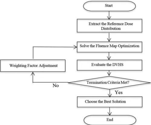
FIG. 1. Flowchart of the proposed algorithm.
model and a unique Pareto surface defined based on the dose distribution concept (calleddose distribution Pareto surface) is generated by the voxel-based model as long as the penalty functionFsatisfies some desirable properties. The dose dis-tribution Pareto surface is much larger than the organ-based Pareto surfaces, and in our previous work38we proved that it
encompasses all the Pareto surfaces generated by the organ-based model using different penalty functions. We also proved that it includes all the plans which are Pareto optimal in terms of the DVH concept. Therefore, the voxel-based model can be employed as a surrogate optimization model especially when our clinically relevant metric is defined based on the DVH. In our previous work, it turns out that the following quadratic voxel-based model is capable of generating almost the entire dose distribution Pareto surface (the entire Pareto surface ex-cluding the so-called nonproperly Pareto optimal points44). So, we employ the following model in this work due to its computational efficiency: minx≥0 σ∈S j∈vσ wj(Djx−rσ)2, (3)
where rσ denotes the prescription dose for the structure σ. Despite the benefits of the voxel-based model, it has a big downside which is the huge number of the parameters. In this paper, we aim to tackle this problem by developing an algo-rithm which takes into account the prior DVH information. In fact, we would like to generate the similar DVHs to the ref-erence ones, which already contain physician approved trade-off information by adjusting the voxel weights.
2.B. Algorithm
To facilitate reading, “the new patient” will refer to the pa-tient for which we look for a plan to generate. That is, “the new patient” can represent the patient in automatic treatment planning or the existing patient with the new geometry in ART replanning. Also, let us refer to the dose distribution Pareto surface of the new patient simply as the “Pareto surface.” We propose an algorithm which iteratively navigates the Pareto surface and projects the plan corresponding to the reference DVHs back on the Pareto surface.
Projecting a plan on the Pareto surface means finding the closest plan on the Pareto surface to the reference plan. It im-plies that, if the reference DVHs are feasible but not Pareto optimal for the new patient, then the projected plan on the Pareto surface would be even better than the reference one in terms of the DVHs; and if the reference DVHs are outside the feasible region of the new patient, meaning it is impossible to generate that plan, then the projected plan on the Pareto sur-face would be similar but not as good as the reference one. In the latter case, the closer the reference plan is to the Pareto surface, the more similar the projected plan would be to the reference one.
Figure1 demonstrates the flow of the algorithm. At first, we find a particular dose distribution corresponding to the reference DVHs (Sec.2.C), referred to as the reference dose distribution. Then, we solve the fluence map optimization problem (3) with some initial weights to get a Pareto opti-mal solution. This solution is evaluated by the metric defined to quantify the difference between its DVHs and the refer-ence DVHs (Sec.2.F). If the termination criteria are not met,
FIG. 2. Extracting the reference dose from the reference DVH for an organ withNvoxels.
among all the permutations of the reference dose distribu-tion that are corresponding to the reference DVHs, we target the closest one to the Pareto solution generated by solving Problem(3) (Sec.2.D). We then project that reference dose distribution back onto the Pareto surface by adjusting the weighting factors (Sec.2.E). We continue the algorithm by solving the fluence map optimization problem with the up-dated weighting factors. When the termination criteria are met, we pick the best solution, in terms of the metric defined to evaluate the DVHs (Sec.2.F), among all the Pareto solu-tions generated by the algorithm.
2.C. Extracting a reference dose distribution from the reference DVHs
Given a set of reference DVHs, our algorithm needs to find out its corresponding dose distribution with the same number of the voxels for each structure as the new patient. A typi-cal dose distribution can be reconstructed by discretizing the volume axis of the DVH uniformly by the number of the vox-els and finding the corresponding dose values. Figure2 illus-trates the process for an organ withNvoxels. In this example, we would have the similar DVH for the new patient’s organ, by spreading the reference dose values ¯d1,d¯2, . . . ,d¯Namong the voxels of the new patient’s organ. It should be noted that DVH is insensitive to the voxel’s spatial location meaning that the reference dose values can be spread among the voxels in any arbitrary way to generate the reference DVH. In another words, if we index the voxels of the new patient’s organ, then any permutation of ¯dcan be assigned to the voxels to generate the reference DVH.
2.D. Nonconvexity issue
After extracting the reference dose distribution from the reference DVHs, we solve Problem (3) with arbitrary
ini-tial weighing factors to get the Pareto optimal solution d0 =Dx0. After obtaining a solution, the weights are updated to guide the DVHs of the current solution toward the reference DVHs. We do not have the DVH directly in our optimiza-tion model, but we have the voxel dose values in Problem
(3). Therefore, we need to change the voxel dose values to make their corresponding DVHs close to the reference ones through updating the weights. The difficulty here is due to the insensitivity of the DVH to the permutation of the dose values in each organ that results in the existence of many paths through which we can change the dose values to get close to the reference DVHs. This problem is known as the nonconvexity problem in radiotherapy optimization. In fact, ifπ(.) :{1, . . . , vσ} → {1, . . . , vσ}denotes an arbitrary per-mutation of the dose values of organσ, thenπ( ¯dσ) would also represent the same DVH and hence we can approach the ref-erence DVH by drivingdσ
0 towardπ( ¯dσ). Now the question that arises here is: “which permutation of the reference dose should be targeted?” To answer this question, we need to con-sider three following possible scenarios regarding the position of the reference DVHs with respect to the feasible solution set of the new patient (the set of all deliverable dose distributions for the new patient).
(i) All permutations of the reference dose are inside the feasible region.
(ii) All permutations of the reference dose are outside the feasible region.
(iii) Some of the permutations of the reference dose are inside the feasible region and the others are outside. For (i), any permutation of the reference dose is possible to be generated since they are all inside the feasible region. They can be even improved by projecting them back onto the Pareto surface. The best plan in this case corresponds to the permutation whose projection provides the most improvement in the reference plan. Figure3(left) clarifies this situation for
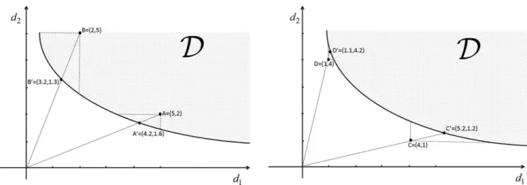
FIG. 3. Projection of different permutations of dose values onto the Pareto surface. (Left: permutations are inside the feasible region): Projecting B results in more improvement in the reference dose. (Right: permutations are outside the feasible region): Projecting D results in less deterioration in the reference dose.
an OAR with two voxels. Points A and B are two different permutations of the reference dose and considered to be the same in terms of the DVH, and A and B are their special projections. It can be seen that Bis better than Ain terms of the DVH which means the more improvement is achieved by projecting B onto the Pareto surface. For the second scenario, any permutation of the reference dose is impossible to be gen-erated and they need to be projected back onto the Pareto surface in order to find the feasible and similar plans to the reference one. The projection in this case would deteriorate the reference dose to make it feasible, and the best plan corre-sponds to the permutation that provides the least deterioration. Figure 3(right) explains this scenario. Points C and D cor-respond to different permutations of the reference dose, and Cand Dare their special projections on the Pareto surface. As can be seen, projecting D results in less deterioration and hence the plan with better DVH. It is obvious that in the third scenario the best plan is obtained by projecting the permuta-tion of the reference dose that is inside the feasible region and results in the most improvement.
Unfortunately, the above procedure is very computation-ally expensive, if not prohibitive. We cope with this issue by iteratively choosing some particular permutation of the refer-ence dose and projecting them back onto the Pareto surface. At each iteration of the algorithm, we target the permutation of the reference dose corresponding to the closest dose dis-tribution to the current Pareto solution. Then, we project the targeted permutation of the reference dose on the Pareto sur-face to get a new Pareto optimal plan. We continue this pro-cess until either the maximum allowed number of iterations is reached or there is not enough improvement in the plan gen-eration. At the end, we pick up the best Pareto optimal plan among all the projected plans on the Pareto surface generated throughout this iteration process, as each iteration is not guar-anteed to produce a better plan than the last. In the rest of this section, we explain how we can find out the closest per-mutation of the reference dose to the current Pareto solution, and in Sec.2.Ewe will elaborate on the projection of the tar-geted plan back on the Pareto surface. Section2.Fintroduces a metric to pick up the best Pareto solution.
Let us consider the initial Pareto solution d0 as a cur-rent solution. For structure σ ∈ S, if ˜π(.) denotes the per-mutation that sorts the vectord0σ in an ascending order [i.e.,
˜
π(dσ
0)=sort(d σ
0)], then according to the following theorem, ˜
π−1( ¯dσ) is the closest permutation of the reference dose to the current solution regardless which p-norm used to measure the distance.
Theorem 1:Forσ ∈S, letdenote the set of all possible permutationsπ(.):{1, . . . , vσ} → {1, . . . , vσ}. Then for every
p∈[1,∞), we have
d0σ−π˜−1( ¯dσ)p ≤d0σ−π( ¯dσ)p ∀π∈. (4)
The proof of this theorem is given in AppendixA. Theorem 1 reveals that, for each structure σ ∈ S, among all the permu-tations π( ¯dσ) of the reference dose that corresponds to the same DVH, ˜π(dσ
0) yields the closest one to the current solu-tion. Now, the dose distribution that we would like to target at a certain iteration of the algorithm can be computed by per-forming the above procedure for each structure. With a slight abuse of notation, we denote the closest dose distribution for all structure by ˜π−1( ¯d). It should be noted that different per-mutations of the reference dose would be targeted at different iterations of the algorithm due to the dependency of the ˜π(.) on the current Pareto solution at each iteration.
2.E. Projection on the Pareto surface
The next step is to project the point ˜π−1( ¯d) back on the Pareto surface of Problem (3). The Pareto surface, here is denoted by F(z) = 0, is a part of the frontier of the set
Z= {z=(Dx−p)2|x≥0}. The frontier ofZ is piecewise quadratic since it is a quadratic transformation of the frontier of the transferred cone (Dx−p) which is piecewise linear. The shape of the Pareto surface depends on the deposition matrix Dand the prescription vector p. There does not ex-ist an efficient way to obtain the Pareto surface, making the projection a challenging problem. We approach this issue by using a quadratic approximation of the Pareto surface.
The projection idea is based on the fact that each point on the Pareto surface corresponds to the set of weighting
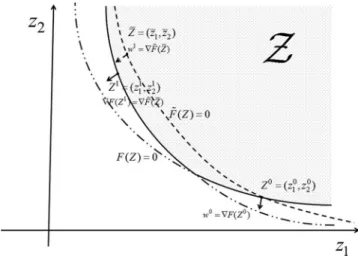
FIG. 4. Illustration of the projection method in a two-dimensional space. The solid line is the Pareto surface, the dashed line is the quadratic surface passing through the initial point and the reference point and its gradient at the reference point would be used as the new weighting factors in the optimiza-tion model.
factors that are the gradient of the Pareto surface (∇F(z)) at that point. Specifically, if we use∇F(z) as the weighting fac-tors in Problem(3), the optimal solution would bez. Now, we use the quadratic surface that passes through the current Pareto solution (d0at the first iteration) and ˜π−1( ¯d) as an ap-proximation of the Pareto surface, and we set the weighting factors of Problem(3) equal to the gradient of this approx-imation of Pareto surface at ˜π−1( ¯d). Then, the optimal so-lution is expected to be on the projection area of the point
˜
π−1( ¯d) on the Pareto surface. Figure4clarifies this process in a two-dimensional space where the point ˜π−1( ¯d) is inside the feasible region. The same behavior can be observed if the point that we want to project is outside the feasible region.
In Fig.4, ¯Z=(¯z1,z¯2) represents the point that is supposed to be projected on the Pareto surface. The Pareto surface, which is a border of the feasible region and is depicted by the solid line, is a piecewise quadratic surface and is denoted here byF(Z)=0. The dashed-dotted lines are the remaining parts of the two quadratic surfaces that make the piecewise quadratic Pareto surface. The dashed line, here is denoted by
˜
F(Z)=0, represents the quadratic surface passing through
the initial point Z0=(z01, z02) and the reference point. The gradient of ˜F(Z) at ¯Zis used as the weighting factors in Prob-lem(3) to obtain the projection of ¯Z on the Pareto surface. Since the weighting factors are corresponding to the gradient of the Pareto surface at the optimal solution, the optimal solu-tion would beZ1 where we have∇F(Z1)= ∇F˜( ¯Z). As can be observed in Fig.4,Z1is located on the projection area of
¯
Zon the Pareto surface. Theorem 2 shows that∇F˜( ¯Z) can be easily approximated from the existing information.
Theorem 2:The new weighting factors utilized to project the closest permutation of the reference dose on the Pareto surface can be approximated as
w1j = ∇jF˜( ¯Z)≈w0j
|d0j−pj|
π˜j−1( ¯d)−pj
∀σ ∈S, j∈vσ. The proof of this theorem is given in Appendix B. By setting the weighting factors equal to w1 in Problem (3)
and solving it, we would get the new dose distribution d1. Then, the above procedure is carried out ond1as the current solution.
2.F. Evaluation of the DVHs
At each iteration of the algorithm, the weighting factors are updated to encourage the DVHs of the current solution (cur-rent DVHs) to approach the reference DVHs. However, we do not directly optimize the distance to the reference DVHs. We need to define an appropriate metric to evaluate the solution quality at each iteration and to pick the best solution among the generated solutions when the algorithm terminates.
We define the metric based on two areas between the ob-tained and the reference DVHs: the areas where the current DVHs are better than the reference DVHs, and the areas where the current DVHs are worse than the reference DVHs. Figure5 illustrates these two types of areas for an organ at risk (left) and a PTV (right). The solid line represents the ref-erence DVH and the dashed line represents the current DVH. The prescription dose for the PTV is shown by a solid verti-cal line in the right plot. For organ at risk,Adepicts the area where the reference DVH is better than the current one and
Bdepicts the area where the current DVH is better. Our first priority is to make A as small as possible, and our second
FIG. 5. Comparing the current DVH and the reference DVH for an OAR (left), and a PTV (right). The solid line represents the reference DVH and the dashed line represents the current DVH.
responding to the areas A and B. Using a small number to reflect different levels of priorities among different objectives is a common approach in optimization.45For PTV, given that the closer dose to the prescription value is preferred,CandE
represent the areas where the reference DVH is better, while
DandFrepresent the areas where the current DVH is better. Therefore, we can define the metric for PTV as
mσ =(mC+mE)−(mD+mF).
Now, we need to combine all organs’ metrics to come up with a single metric to quantify the current DVHs. While there are many ways to do that, we take the maximum value among all the organs’ metrics
m=maxσ∈Smσ, (5)
where mσ is a metric corresponding to the structure σ. To some extent, this metric would choose the plan for which the deviation to the reference plan is uniformly distributed among all the organs. To have a better convergence behavior for the algorithm in terms of the above metric, it is better to reflect the desire of distributing the deviation uniformly among the organs in the algorithm. Toward this end, we penalize each organ weights proportional to its deviation mσ to the refer-ence DVH. It can be done through the following weight ad-justment: wj1=w0j ⎛ ⎝1+ mσ max σ∈S|mσ| ⎞ ⎠∀j ∈vσ, σ ∈S.
3. EXPERIMENTS AND RESULTS
In this section, we provide three different case studies. All of them are IMRT cases with seven equispaced beam angles. The first case is designed to test the capability of the algo-rithm to project a reference plan on the Pareto surface, and we use Matlab as our computational framework for this case. The second and the third case studies represent the applications of the algorithm for adaptive radiotherapy replanning and au-tomatic treatment planning. We use our inhouse GPU-based research planning system (SCORE) to run the algorithm and demonstrate the results for these two cases. We set beamlet size and voxel size to 0.5 ×0.2 and 0.2×0.2×0.25 cm3, respectively. We cannot afford solving the optimization prob-lem including all the voxels and so we just pick out some of them by downsampling process. However, to make the second and the third case studies more realistic, the final dose calcu-lation on all the voxels, including MLC transmission, will be performed after optimization. Moreover, since we aim to eval-uate the performance of the proposed optimization algorithm, in the following we will just mention the number of the vox-els used in optimization model and the time spent to solve the optimization problem.
ble DVHs), (2) the reference DVHs are outside the feasible region (infeasible DVHs). We will show that the algorithm generates a plan with DVHs better than the reference ones for the first scenario, while it finds a plan with DVHs worse than, but similar to, the reference ones for the second scenario.
In order to get the feasible and infeasible sets of the DVHs, we first generated a plan by solving Problem(3)with a set of the weighting factors, which yields a plan that is Pareto opti-mal in terms of the DVHs,38 and then we manipulated them.
An infeasible plan can be obtained by improving the DVH curves of the Pareto optimal plan (shifting the OAR DVHs toward left and PTV DVH toward prescription dose), and a feasible plan can be generated by worsening the DVHs of the Pareto optimal plan.
Figures6and7are regarding the feasible reference DVHs shown by the solid lines. The dotted lines in Fig. 6 depict the result of the algorithm. As can be seen, the DVHs gener-ated by the algorithm are better than the reference ones due to the feasibility of the reference DVHs. In fact, the algorithm projects the feasible reference plan on the Pareto surface re-sulting in a better plan. It took us 10.6 s to get this plan. Figure 7 investigates the nonconvexity issue that may lead to local optimality. For this purpose, we ran the algorithm 100 times with randomly generated initial weighting factors, and then we picked the best (dotted lines) and the worst (dashed lines) solutions with respect to our metric introduced in Eq. (5). It seems that the local optimality is not a big is-sue for this case, especially since both plans are better than the reference one. In fact, the algorithm projects the refer-ence plan on the Pareto surface regardless the initial solution which implies that all 100 plans are Pareto optimal and on the projection area of the reference plan. However, given that the algorithm started from different points on the Pareto surface, it ends up in different parts of the projection area.
Figures8and9deal with the infeasible reference DVHs. Figure8 shows that the algorithm is able to generate a plan that, although worse than the reference plan, is close to it. The computation time is 7.4 s in this case. Figure 9 exam-ines the local optimality issue by running the algorithm for 100 times with randomly generated initial weights and illus-trates the best and the worst plans. Again, the local optimality does not seem to be a big problem.
3.B. Adaptive radiotherapy replanning for a head and neck case
The application of the proposed algorithm in adaptive ra-diotherapy replanning is illustrated in this section with a head and neck case that has been treated previously at UCSD Moores Cancer Center. The number of the voxels and beam-lets for this patient are 20 758 and 13 934, respectively. The
FIG. 6. Dotted line: The result of the algorithm. Solid line: The feasible reference DVHs.
FIG. 7. Investigating the local optimality issue: The algorithm has been run 100 times with randomly generated starting points, and the dotted and the dashed lines represent the best and the worst solutions, respectively. Solid lines are the feasible reference DVHs.
FIG. 9. Investigating the local optimality issue: The algorithm has been run 100 times with randomly generated starting points, and the dotted and the dashed lines represent the best and the worst solutions, respectively. Solid lines are the infeasible reference DVHs.
optimization algorithm took 11.6 s to run on our inhouse GPU-based research planning system (SCORE).
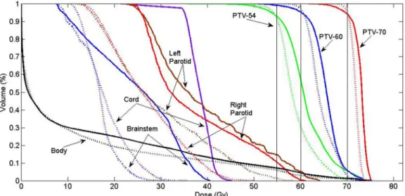
The solid line in Fig.10depicts the original clinical plan developed on the patient’s original geometry. The dotted line demonstrates the result of our algorithm, after final dose cal-culation, when we used the original plan as a reference on the patient’s new geometry. As can be seen, the optimal plan for the patient’s new geometry is better than the original plan almost everywhere. We looked at the result of the algorithm right after the optimization, before final dose calculation, and we found out the result is even better. It means that the origi-nal plan is inside the feasible region corresponding to the pa-tient’s new geometry and so the algorithm is able to generate a better plan by projecting the original plan back on the Pareto surface. The significant improvement in plan quality in this figure can be explained with two main possible reasons: (1) the patient’s geometry has been changed in a way that made
the original plan located far inside the feasible region of the new geometry leading to the substantial improvement by pro-jecting that plan on the Pareto surface, (2) the proposed al-gorithm explores a much larger voxel-based Pareto surface of the new geometry that can help to find out a plan with bet-ter trade-offs. Another theoretically possible reason (proba-bly unlikely) is that the original plan generated by the com-mercial software is not a Pareto optimal plan for the original geometry.
Figure11compares the original plan delivered on the pa-tient’s new geometry (solid line) with the new plan generated by the algorithm (dotted line). This figure verifies the bene-fit of using the proposed algorithm instead of delivering the original plan on the new geometry. If we do not consider the possible adverse effect of the final dose calculation and MLC transmission, since the original plan delivered on the new ge-ometry is a feasible plan and always inside the feasible region,
FIG. 11. Solid line: The original plan delivered on the patient’s new geometry. Dotted line: The result of the algorithm.
the plan generated by the algorithm would be always better than this plan.
Figure12 compares the dose distribution of the original plan delivered on the patient’s new geometry (a) and (c) with the new plan generated by the algorithm (b) and (d). The dose distribution also verifies the improvement in plan qual-ity in terms of both tumor coverage and healthy tissue sparing. However, since the dose distribution was not part of the op-timization process, we cannot draw a solid conclusion about the quality of the dose distribution at this moment. This tech-nique’s effects on the dose distribution need either more
ex-perimental study or a change to explicitly consider dose dis-tribution quality as part of the optimization model.
3.C. Automatic treatment planning for a prostate case
With this example we demonstrate how the proposed al-gorithm can be used for automatic treatment planning. We assume that there is a new patient that we want to treat by using a library of plans of already treated patients with sim-ilar medical conditions. We use a prostate case that has been treated previously at UCSD Moores Cancer Center as a new
FIG. 13. Solid line: The DVHs of the most similar patient as the reference DVHs. Dotted line: The result of the algorithm by using the solid line as reference.
patient. The number of the voxels and beamlets for this case are 22 229 and 3412, respectively. First, we went through the library of 99 treated prostate cases and found the most similar one to the new patient in terms of organs geometry.46This step
is accomplished by employing some machine learning tech-niques to find out a similarity function that uses some geo-metric features as inputs (e.g., organ/PTV volume, organ/PTV overlapping volume, Dice index, and mutual information be-tween a pair of two organs/PTVs/intersections) and DVH ilarity as an output. Then, we used the DVHs of the most sim-ilar patient as the reference DVHs in the algorithm to generate a plan for the new patient.
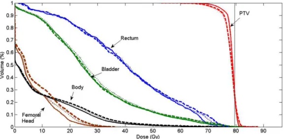
The solid line in Fig. 13 illustrates the reference DVHs and the dotted line represents the result of the algorithm for the new patient. It can be seen that the result is better that the reference DVHs everywhere except for rectum which is due to the final dose calculation and MLC transmission. It means that the reference DVHs is inside the feasible region of the new patient. It took us 7.2 s to solve the optimization problem
and find the plan for the new patient in our inhouse planning system.
Figure14compares the clinical plan that has been deliv-ered for patient treatment (solid line) to the result of the au-tomatic treatment planning (dotted line). These two plans are not exactly the same, but they both provide clinically accept-able trade-offs between different organs.
4. DISCUSSION AND CONCLUSION
The benefits of using the voxel-based model have been dis-cussed before by many authors, however, determining the nu-merous parameters in the model continues to be a challenge in practice. In this paper, we studied how the prior DVH infor-mation that exists in automatic treatment planning and ART replanning can be employed as guidance to tune treatment plan optimization parameters.
We proposed an algorithm that is capable of adjust-ing voxel weights automatically and navigatadjust-ing the dose
FIG. 14. Solid line: The original clinical plan delivered for patient treatment. Dotted line: The result of the algorithm by using the automatic treatment planning technique.
distribution Pareto surface to approach a plan with DVHs similar to the given DVHs. The proposed algorithm itera-tively approximates the piecewise quadratic Pareto surface with a quadratic one to project the given DVHs back on the Pareto surface. The nonconvexity issue that comes from the insensitivity of the DVH to the spatial properties of the voxels has been handled by iteratively picking some partic-ular permutations of the dose values resulting in the same DVH. The local optimality turned out to be not a big prob-lem based on our limited experience; however, more experi-mental study needs to be done in this direction to draw a solid conclusion.
We discussed the potential applications of the proposed al-gorithm in automatic treatment planning and ART replanning. However, the natural question that arises here is “what if the plan generated by the algorithm for automatic treatment plan-ning or ART replanplan-ning does not satisfy some of the clini-cian’s criteria in terms of the DVH or dose distribution?” In our next work, we will show how the clinician can interac-tively tune the DVH curves and dose distribution of the gen-erated plan to make the plan satisfactory.
The capability of the algorithm to project a feasible and infeasible reference plan to the Pareto surface may beg the question of “what if we put an ideal DVH (zero dose in normal tissues and prescribed dose in tumor) or a very lousy DVH as a reference?” The answer to this question lies in the fact that, while the algorithm tries to project a reference plan on the projection area, it cannot guide the reference plan toward a particular part of the projection area. In other words, when the reference needs to be improved (feasible reference) or com-promised (infeasible reference) to make the projection, we do not have too much control on the way that improvement or compromise is done. This is not going to be a problem if the reference plan is close to the Pareto surface since the projec-tion area would be relatively small. However, if the reference plan is far from the Pareto surface, like the ideal or very lousy reference, then the projection area would be quite big and the result of the algorithm could be unpredictable. This is actu-ally the main reason that for ART and automatic treatment planning we pick some reference plans that are expected to be close to the Pareto surface.
Finally, we would like to mention that we picked the DVH to guide the optimization process due to its flexibility and in-dependence to the geometry of the patient; however, there are other clinically relevant indices that physicians care about and need to be taken into account in optimization process in order to produce a fully satisfactory plan. We believe that this will be a good direction for our future work.
APPENDIX A: PROOF OF THEOREM 1
First, we prove the following inequality:
||sort(a)−sort(b)||p≤ ||a−b||p, (A1) wherea,b∈Rn. The proof is by induction onn. Forn=2, the proof is intuitive and we just need to investigate different relative positions ofaandb. Assume that the inequality holds forn=kwherek≥2. For n=k+1, let us denote sort(a)
byc=(c1, . . . ,ck+1) and sort(b) byd=(d1, . . . ,dk+1). Since (k+1)≥3, it can be readily shown that there existi∈{1, . . . ,k+1} such thatai>c1 andbi >d1. In fact,aiandbi are considered not to be the smallest components ofaandb. Now, we have ||a−b||pp = ||(a1, . . . , ai−1, ai+1, . . . , ak+1) −(b1, . . . , bi−1, bi+1, . . . , bk)||pp+|ai−bi|p, (A2) ≥ ||sort(a1, . . . , ai−1, ai+1, . . . , ak+1) −sort(b1, . . . , bi−1, bi+1, . . . , bk)||pp+ |ai−bi|p (A3) = |c1−d1|p+ ||w−v||pp. (A4)
Inequality(A3) is obtained from Eq. (A2) by applying the induction assumption. To get Eq.(A4)from Eq.(A3), we just need to consider thatc1 andd1 are the smallest components ofaandb, and they are not equal toaiandbi.wandvare the names for the remaining elements. Now, sincewandvhave
kcomponents, we can employ the induction assumption for ||w−v||pp and have
|c1−d1|p+ ||w−v||pp ≥ |c1−d1|p+ ||sort(w)
−sort(v)||pp = ||sort(a)−sort(b)||pp. (A5)
Inequality(A1)can be obtained from Eqs.(A2)to(A5)and by applying the functionf(x)=xp1 to the both sides of the inequality.
Now, the original inequality (4) can be proved by using inequality(A1). For an arbitraryπ ∈ , we seta=dσ
0 and
b=π( ¯dσ). Applying Eq.(A1)and considering that ¯dσ is a sorted vector and ˜π( ¯dσ
0)=sort( ¯d σ
0), we have
π˜d0σ −d¯σp ≤ ||d¯0−π( ¯dσ)||p.
Given that the norm is not sensitive to the permutation, we have
d0σ−π˜−1( ¯dσ)p =π˜d0σ −d¯σp
which completes the proof.
APPENDIX B: PROOF OF THEOREM 2
Since the quadratic function is an increasing function, the Pareto surface of Problem(3) is exactly the quadratic trans-formation of the Pareto surface of the following problem:
minx≥0w.|Dx−r|. (B1)
It means,zbelongs to the Pareto surface of Problem(3)if and only if√z belongs to the Pareto surface of Problem (B1). On the other hand, the Pareto surface of Problem (B1) is piecewise linear. Therefore, if F(z) = 0 denotes the Pareto surface of Problem (3), then there exists a set of vectors {αi}ni=1for which we haveF(z)=α.
√
z−1 forα∈ {αi}ni=1. Now, we approximate F(z) with ˜F(z)=α.˜ √z−1 where
Using the approximation∇F˜(z0)≈ ∇F(z0)=w0and tak-ing into account that z0 =(d0 −p)2and ¯z=( ˜π−1( ¯d)−p)2 would complete the proof.
a)Author to whom correspondence should be addressed. Electronic mail: [email protected]
1M. J. Williams, M. Bailey, D. Forstner, and P. E. Metcalfe, “Multicentre quality assurance of intensity-modulated radiation therapy plans: A precur-sor to clinical trials,”Australas. Radiol.51, 472–479 (2007).
2I. J. Das, C.-W. Cheng, K. L. Chopra, R. K. Mitra, S. P. Srivastava, and E. Glatstein, “Intensity-modulated radiation therapy dose prescription, recording, and delivery: Patterns of variability among institutions and treat-ment planning systems,”J. Natl. Cancer Inst.100, 300–307 (2008). 3H. T. Chung, B. Lee, E. Park, J. J. Lu, and P. Xia, “Can all centers plan
intensity-modulated radiotherapy (IMRT) effectively? an external audit of dosimetric comparisons between three-dimensional conformal radiother-apy and IMRT for adjuvant chemoradiation for gastric cancer,”Int. J. Ra-diat. Oncol., Biol., Phys.71, 1167–1174 (2008).
4S. Breedveld, P. R. M. Storchi, M. Keijzer, A. W. Heemink, and B. J. M. Heijmen, “A novel approach to multi-criteria inverse planning for IMRT,”Phys. Med. Biol.52, 6339–6353 (2007).
5S. Breedveld, P. R. M. Storchi, and B. J. M. Heijmen, “The equivalence of multi-criteria methods for radiotherapy plan optimization,”Phys. Med. Biol.54, 7199–7209 (2009).
6S. Breedveld, P. R. M. Storchi, P. W. J. Voet, and B. J. M. Heijmen, “iCycle: Integrated, multicriterial beam angle, and profile optimization for genera-tion of coplanar and noncoplanar IMRT plans,”Med. Phys.39, 951–963 (2012).
7P. W. J. Voet, M. L. P. Dirkx, S. Breedveld, D. Fransen, P. C. Levendag, and B. J. M. Heijmen, “Toward fully automated multicriterial plan generation: A prospective clinical study,”Int. J. Radiat. Oncol., Biol., Phys.85, 866– 872 (2013).
8X. Zhang, X. Li, E. M. Quan, X. Pan, and Y. Li, “A methodology for au-tomatic intensity-modulated radiation treatment planning for lung cancer,”
Phys. Med. Biol.56, 3873–3893 (2011).
9V. Chanyavanich, S. K. Das, W. R. Lee, and J. Y. Lo, “Knowledge-based IMRT treatment planning for prostate cancer,”Med. Phys.38, 2515–2522 (2011).
10B. Wu, F. Ricchetti, G. Sanguineti, M. Kazhdan, P. Simari, R. Jacques, R. Taylor, and T. McNutt, “Data-driven approach to generating achiev-able dose–volume histogram objectives in intensity-modulated radiother-apy planning,”Int. J. Radiat. Oncol., Biol., Phys.79, 1241–1247 (2011). 11D. Yan, F. Vicini, J. Wong, and A. Martinez, “Adaptive radiation therapy,”
Phys. Med. Biol.42, 123–132 (1997).
12R. Mohan, X. Zhang, H. Wang, Y. Kang, X. Wang, H. Liu, K. K. Ang, D. Kuban, and L. Dong, “Use of deformed intensity distributions for on-line modification of image-guided IMRT to account for interfractional anatomic changes,” Int. J. Radiat. Oncol., Biol., Phys. 61, 1258–1266 (2005).
13L. E. Court, L. Dong, A. K. Lee, R. Cheung, M. D. Bonnen, J. O’Daniel, H. Wang, R. Mohan, and D. Kuban, “An automatic CT-guided adaptive radiation therapy technique by online modification of multileaf collimator leaf positions for prostate cancer,”Int. J. Radiat. Oncol., Biol., Phys.62, 154–163 (2005).
14Y. Feng, C. Castro-Pareja, R. Shekhar, and C. Yu, “Direct aperture defor-mation: An interfraction image guidance strategy,”Med. Phys.33, 4490– 4498 (2006).
15L. E. Court, R. B. Tishler, J. Petit, R. Cormack, and L. Chin, “Automatic on-line adaptive radiation therapy techniques for targets with significant shape change: A feasibility study,”Phys. Med. Biol.51, 2493–2501 (2006). 16A. Mestrovic, M.-P. Milette, A. Nichol, B. G. Clark, and K. Otto, “Direct
aperture optimization for online adaptive radiation therapy,”Med. Phys.
34, 1631–1646 (2007).
IMRT plans for adaptive radiation therapy,”Phys. Med. Biol.53, 673–691 (2008).
20C. Men, X. Jia, and S. B. Jiang, “GPU-based ultra-fast direct aperture opti-mization for online adaptive radiation therapy,”Phys. Med. Biol.55, 4309– 4319 (2010).
21M. Langer and J. Leong, “Optimization of beam weights under dose-volume restrictions,”Int. J. Radiat. Oncol., Biol., Phys.13, 1255–1260 (1987).
22M. Langer, R. Brown, M. Urie, J. Leong, M. Stracher, and J. Shapiro, “Large scale optimization of beam weights under dose-volume restric-tions,”Int. J. Radiat. Oncol., Biol., Phys.18, 887–893 (1990).
23Y. Censor, M. D. Altschuler, and W. D. Powlis, “On the use of Cimmino’s simultaneous projections method for computing a solution of the inverse problem in radiation therapy treatment planning,”Inverse Probl.4, 607– 623 (1988).
24S. M. Morrill, R. G. Lane, J. A. Wong, and I. I. Rosen, “Dose-volume con-siderations with linear programming optimization,”Med. Phys.18, 1201– 1210 (1991).
25P. S. Cho, S. Lee, R. J. M. Ii, S. Oh, S. G. Sutlief, and M. H. Phillips, “Opti-mization of intensity modulated beams with volume constraints using two methods: Cost function minimization and projections onto convex sets,”
Med. Phys.25, 435–443 (1998).
26S. V. Spirou and C. S. Chui, “A gradient inverse planning algorithm with dose-volume constraints,”Med. Phys.25, 321–321 (1998).
27D. Michalski, Y. Xiao, Y. Censor, and J. M. Galvin, “The dose–volume constraint satisfaction problem for inverse treatment planning with field segments,”Phys. Med. Biol.49, 601–616 (2004).
28H. E. Romeijn, R. K. Ahuja, J. F. Dempsey, and A. Kumar, “A new linear programming approach to radiation therapy treatment planning problems,”
Operations Res.54, 201–216 (2006).
29Y. Zhang and M. Merritt, “Dose-volume-based IMRT fluence optimization: A fast least-squares approach with differentiability,”Linear Algebra Appl.
428, 1365–1387 (2008).
30M. Zarepisheh, M. Shakourifar, G. Trigila, P. S. Ghomi, S. Couzens, A. Abebe, L. Noreña, W. Shang, S. B. Jiang, and Y. Zinchenko, “A moment-based approach for DVH-guided radiotherapy treatment plan op-timization,”Phys. Med. Biol.58, 1869–1887 (2013).
31C. Cotrutz and L. Xing, “Using voxel-dependent importance factors for in-teractive DVH-based dose optimization,”Phys. Med. Biol.47, 1659–1669 (2002).
32C. Cotrutz and L. Xing, “IMRT dose shaping with regionally variable penalty scheme,”Med. Phys.30, 544–544 (2003).
33C. Wu, G. H. Olivera, R. Jeraj, H. Keller, and T. R. Mackie, “Treatment plan modification using voxel-based weighting factors/dose prescription,”
Phys. Med. Biol.48, 2479–2491 (2003).
34Y. Yang and L. Xing, “Inverse treatment planning with adaptively evolving voxel-dependent penalty scheme,”Med. Phys.31, 2839–2839 (2004). 35Z. Shou, Y. Yang, C. Cotrutz, D. Levy, and L. Xing, “Quantitation of the
a priori dosimetric capabilities of spatial points in inverse planning and its significant implication in defining IMRT solution space,”Phys. Med. Biol.
50, 1469–1482 (2005).
36C. Holdsworth, M. Kim, J. Liao, and M. Phillips, “The use of a multiob-jective evolutionary algorithm to increase flexibility in the search for better IMRT plans,”Med. Phys.39, 2261–2274 (2012).
37N. Li, M. Zarepisheh, A. Uribe-Sanchez, K. Moore, Z. Tian, X. Zhen, Y. J. Graves, Q. Gautier, L. Mell, L. Zhou, X. Jia, and S. Jiang, “Automatic treatment plan re-optimization for adaptive radiotherapy guided with the initial plan DVHs,” Phys. Med. Biol. 58, 8725–8738 (2013).
38M. Zarepisheh, A. Uribe-Sanchez, N. Li, X. Jia, and S. Jiang, “A multi-criteria framework with voxel-dependent parameters for radiotherapy treat-ment plan optimization,”Med. Phys.41, 041705 (10pp.) (2014). 39H. E. Romeijn, J. F. Dempsey, and J. G. Li, “A unifying framework for
multi-criteria fluence map optimization models,” Phys. Med. Biol. 49, 1991–2013 (2004).
40A. L. Hoffmann, D. den Hertog, A. Y. D. Siem, J. H. A. M. Kaanders, and H. Huizenga, “Convex reformulation of biologically-based multi-criteria intensity-modulated radiation therapy optimization including fractionation effects,”Phys. Med. Biol.53, 6345–6362 (2008).
41D. Craft, T. Halabi, and T. Bortfeld, “Exploration of tradeoffs in intensity-modulated radiotherapy,”Phys. Med. Biol.50, 5857–5857 (2005). 42M. L. Kessler, D. L. McShan, M. A. Epelman, K. A. Vineberg, A. Eisbruch,
T. S. Lawrence, and B. A. Fraass, “Costlets: A generalized approach to cost functions for automated optimization of IMRT treatment plans,”Optim. Eng.6, 421–448 (2005).
43P. Xia, N. Yu, L. Xing, X. Sun, and L. J. Verhey, “Investigation of using a power function as a cost function in inverse planning optimization,”Med. Phys.32, 920–920 (2005).
44M. Ehrgott,Multicriteria optimization(Springer Verlag, Berlin, 2005). 45M. Zarepisheh and E. Khorram, “On the transformation of lexicographic
nonlinear multiobjective programs to single objective programs,” Math. Methods Operations Res.74, 217–231 (2011).
46M. Karimi, N. Li, M. Zarepisheh, L. Cervino, X. Jia, K. Moore, and S. Jiang, “Selecting reference patients for automatic treatment planning us-ing multiple geometrical features,”Med. Phys.40, 379 (2013) (Abstract).