Survival analysis approaches for prostate cancer.

(1)

Survival Analysis Approaches for Prostate Cancer

By

Eman Alhasawi

A thesis submitted in partial fulfillment

of the requirements for the degree of

Master of Science (MSc) in Computational Sciences

The Faculty of Graduate Studies

Laurentian University

Sudbury, Ontario, Canada

(2)

THESIS DEFENCE COMMITTEE/COMITÉ DE SOUTENANCE DE THÈSE Laurentian Université/Université Laurentienne

Faculty of Graduate Studies/Faculté des études supérieures Title of Thesis

Titre de la thèse Survival Analysis Approaches for Prostate Cancer

Name of Candidate

Nom du candidat Alhasawi, Eman

Degree Diplôme Master of Science

Department/Program Date of Defence

Département/Programme Computational Sciences Date de la soutenance April 15, 2015

APPROVED/APPROUVÉ

Thesis Examiners/Examinateurs de thèse:

Dr. Kalpdrum Passi

(Supervisor/Directeur de thèse)

Dr. Mazen Saleh

(Committee member/Membre du comité)

Dr. Hafida Boudjellaba

(Committee member/Membre du comité)

Approved for the Faculty of Graduate Studies Approuvé pour la Faculté des études supérieures Dr. David Lesbarrères

M. David Lesbarrères

Dr. Chakresh Jain Acting Dean, Faculty of Graduate Studies (External Examiner/Examinateur externe) Doyen intérimaire, Faculté des études supérieures

ACCESSIBILITY CLAUSE AND PERMISSION TO USE

I, Eman Alhasawi, hereby grant to Laurentian University and/or its agents the non-exclusive license to archive and make accessible my thesis, dissertation, or project report in whole or in part in all forms of media, now or for the duration of my copyright ownership. I retain all other ownership rights to the copyright of the thesis, dissertation or project report. I also reserve the right to use in future works (such as articles or books) all or part of this thesis, dissertation, or project report. I further agree that permission for copying of this thesis in any manner, in whole or in part, for scholarly purposes may be granted by the professor or professors who supervised my thesis work or, in their absence, by the Head of the Department in which my thesis work was done. It is understood that any copying or publication or use of this thesis or parts thereof for financial gain shall not be allowed without my written permission. It is also understood that this copy is being made available in this form by the authority of the copyright owner solely for the purpose of private study and research and may not be copied or reproduced except as permitted by the copyright laws without written authority from the copyright owner.

(3)

ii

Abstract

Survival time has become an essential outcome of clinical trial, which began to emerge among the latter half of the 20th century. A present study was carried out on the survival analysis for patients with prostate cancer. The data was obtained from Memorial Sloan Kettering where each sample was collected from the recipients of the treatment of radical prostatectomy. The Kaplan-Meier method was used to obtain and estimate the survival function and median time among the primary and metastatic tumor of prostate cancer. Results showed that the metastatic tumor has a poor survival rate compared to the primary tumor, which give us a hint that primary tumor has a higher probability of surviving. The log-rank test was used to test the differences in the survival curves. The results showed that the difference in survival rate between the patients of the two groups of tumor was significant with a p-value of 4.44e-15. The second approach was based on the efficiency of cox proportional hazards model and parametric model. Some criteria of residuals were used for judging the goodness of fit among the candidate models. The cox proportional hazard (PH) model provided an effective covariate on the hazard function. As a result of cox PH model, the influence of standard clinical prognostic factors is based on the hazard rate of prostate cancer patients. These prognostic factors are: prostate specific antigen (PSA) level at diagnosis, tumor size, Secondary Gleason grade, and Gleason score which is helpful to determine the treatment. The Gleason score [HR 4.835, 95% CI 2.7847- 8.3937, p=2.20E-08] has the most significant progression-associated prognosticators and reveal to be an effective criteria leading to death in prostate cancer. The Accelerated Failure Time (AFT) was applied to the data with four distortions. AFT with Weibull distortions was chosen to be the best model for our data by testing the AIC.

(4)

iii

Acknowledgements

I would like to thank my God, who got me this far; who blessed me with the right people to help me during the different stages of my study.

It gives me great pleasure to express my deepest respect and sincere thanks to my advisor Professor Kalpdrum Passi for his encouragement, valuable suggestions, discussion and guidance throughout my graduate studies. He continually and convincingly conveyed a spirit of adventure in regard to research. He was patient with my writing style and taught me how to explain my thoughts and present them clearly in writing. Without his guidance and persistent help this thesis would not have been possible.

I am deeply indebted to my committee Dr. Hafida Boudjellaba who always found time to provide constructive feedback to my thoughts. She provided me with technical support and become more of a mentor friend, than a professor. She answered my detailed oriented questions and helped me progress. I am grateful for her tremendous help at the initial stages of developing my thesis project.

I would like to express my regards and thanks to Dr. Mazen Saleh, a member of my supervisory committee for reading my thesis and providing valuable feedback on my thesis.

I would like to send my appreciation and respects to Dr. Peter Adamic for his help and suggestions.

It is with immense gratitude to thank my family for their love, helps, and supports, especially my parents Ahmed Ali and Anisah Ahmed for being supportive and helping me get all the annoying little things done, my wonderful brother, Ali for supporting me in my pursuit of this degree. I would like to express my gratefulness towards my sisters Azhar and Asia who were always there for me and cheering me on all situations.

I am also grateful to all my friends here in Sudbury and my friends in Saudi Arabia for their encouragement and to help change my career path. I couldn’t have achieved this without their help.

(5)

iv

I wish to express my deepest appreciation to the King Abdullah, for giving Saudi women the scholarship to complete studying. I recognize that thesis would not have been possible without the financial assistance of Saudi Cultural Bureau in Canada and the Saudi Ministry of Higher Education.

(6)

v

This thesis is dedicated to

My family and friends,

Without whose support and inspiration

I would never have had the courage to follow my dreams.

I love you and I miss you.

(7)

vi

List of figure

Figure page

1.1 Illustration of left, right and interval censoring (Aaserud,2011)……….…… 10 1.2 Generally used AFT in survival analysis(Sewalem, 2012).…….……….………. 13 1.3 The following steps were providing of analyzing the clinical trial for survival analysis in

R………..14

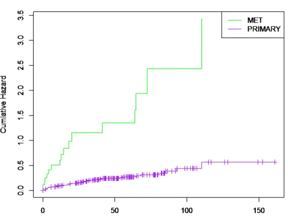
3.1 Description illustrated of the clinical data for prostate cancer..……….……… 22 4.1 Survival curve of two tumor groups (primary and Met) for the prostate data in table 4.1… 43 4.2 Shows the lines for the prostate cancer data with two types of tumors……….……… 45 4.3 Survival times of patients with primary tumor according to Gleason grade.…..…... 51 4.4 The Cox proportional hazard PH with error bars show 95% confidence

intervals...……….………..………….…....………... 53 4.5 Schoenfeld residuals for each explanatory variable versus transformed time in a model fit ...to the prostate cancer data. ...………...….………..… 55 4.6 Cumulative hazard plot of the Cox-Snell residual for Cox PH model to indicate the overall

model………...…….……….……….……….….. 56 4.7 Plot of martingale residuals vs. covariates. ………….……….………...…. 58 4.8 Deviance residuals consist of information about the influential and outlier data. ……...… 60 4.9 Cumulative hazard plot of the Cox-Snell residual for Weibull AFT model. …………...… 63

(10)

ix

List of Table

Table page

1.1 Four stages of Tumor (University of Maryland). .………...…………..…. 6

1.2 The survival time………...…...………... 8

1.3 The main model in survival analysis. ……….…..……...………...…… 13

3.1 Clinical data of prostate cancer. . ……….…..……...……..………..….……. 21

Descriptive statistics for the distributions of the variables (Taylor, 2010)…………...… 24

4.1 Initial sorted table for Kaplan- Meier and Log- Rank analysis………...… 41

4.2 Calculation for the K-M estimate of the survival function for primary type of tumor ………..……… 46

4.3 Calculation for the K-M estimate of the survival function for Met type of tumor………..……..……….…….. 47

4.4 Calculation for the log- rank test to compare tumor groups for the data in Table 4.1...48

4.5 The Cox’s proportional hazards analysis for the prostate cancer patient………..……... 51

4.6 The hazard rate.………....….. 51

4.7 Scaled Schoenfeld Residuals of Significant Covariates on the PH………. 54

4.8 Deviance residuals against the risk score………..…….. 59

4.9 The log-likelihoods and Akaike Information Criterion (AIC) in the AFT models………. 61

(11)

x

List of APPENDIX

Appendix page Appendix A ... Error! Bookmark not defined. Appendix B ... 78

Appendix C: ... 81

(12)

xi

Abbreviations

HR hazard ratio

PH Promotional hazard CI confidence interval PSA prostate specific antigen RP radical prostatectomy Mets metastasis

GS Gleason score

BCR biochemical recurrence K-M Kaplan–Meier

AIC Akaike’s information criterion AFT Accelerated failure time

MSKCC Memorial Sloan Kettering Cancer Center PathStage Tumor stage

PathGGS Combined Gleason score PathGG1 Secondary Gleason grade PreDxBxPSA PSA level at diagnosis

BCR_FreeTime Time until recurrence (months)

BCR_Event Recurrence event (as defined by rise of PSA level) Race Patient race

(13)

xii BxGGS Biopsy combined Gleason score BxGG1 Biopsy primary Gleason grade BxGG2 Biopsy secondary Gleason grade ClinT_Stage Clinical Tumor stage

SMS Surgical margin status ECE Extra-capsular extension SVI Seminal vesicle invasion LNI Lymph node involvement Ng/ml nanogram/millilitre IQR interquartile range

(14)

1

Chapter1

Introduction

This chapter starts with an essential issue in health, which is cancer. Specially, a review of prostate cancer with the related prognostic factors is presented. An overview of survival analysis is discussed along with important models that are relevant to the present study.

1.1 Prostate Cancer

Cancer is a term used for group of diseases where the cells have abnormal behavior of growth and division. There are more than 100 different types of cancer. The prostate cancer originates in prostate gland in the male reproductive system. Its function is producing fluid that protects and nourishes sperm cells in semen. The cancer cell can spread in different ways, such as through tissue, lymph system, and blood (National Cancer Institute). Prostate cancer is the second most common malignant cancer causing death in men, after lung cancer, and its incidence increases with age. Compared to other cancers, men with prostate cancer can live many years, since it grows slowly (Prostate Cancer Canada). Fortunately, prostate cancer in early stages of the disease, in half of the new cases, is still confined to the prostate. However, there are a significant number of cases of aggressive prostate cancers that can be very devastating. The cell of prostate cancer can spread to other parts of the body, which is called metastasis, such as the bones and lymph nodes.

The numbers of new cases of prostate cancer diagnosed each year in the US are approximately 220,000 and 30,000 of them die of the disease. In addition, the number of new cases of prostate cancer in 2013 was 238,590, and the number of deaths was 29,720. In 2014, the new cases of prostate cancer diagnosed were about 233,000 and about 29,480 of them died (American Cancer Society).

Research has identified the fundamental risk factors of prostate cancer; they are: age, race/ ethnicity, and family history. Among these, age has been found to be the most important factor, especially in older men over 60. It is found in the research that surgical radical prostatectomy (RP) had better results in young men than in older men. Literature has proved that African Americans have higher risk of prostate cancer, approximately 60%, than whites (Litwin et al.,

(15)

2

2000). If close family members, such as parents and grandparents, have had the disease, it is more likely that their children would have it (Prostate Cancer Canada). There are other possible factors that may increase the risk such as diet, body mass index (BMI), concomitant medical conditions, and hormone profiles,

1.1.1 Tumors

Primary Tumor

When the cancer has begun in any organ or tissue, the original tumor site is referred as the primary tumor or cancer.

Metastatic Tumor

Metastasis is a process that refers to the spread of cancer. This process can be understood as cancer cells breaking away from the primary tumor in the body and then entering the bloodstream or lymphatic system. A metastatic tumor or a metastasis is a tumor that is made via metastatic cancer cells. The cells can spread to the adrenal gland, bones, liver, and lungs. Metastatic cancer occurs exclusively in male patients, affecting the prostate. While the cancer can cause severe pain in patients, the depletion of testosterone or ingestion of medications, can improve the patient’s urinary function and relieve some pain and discomfort.

Metastatic cancer is considered to be similar to the primary cancer. In many cases of the metastatic, if it is found as the first tumor, then the primary can also be found. However, some patients can have the metastatic without the primary tumor (National Cancer Institute). A pathologist examines to determine if a cancer is a primary or a metastatic tumor.

1.1.2 Prognostic Factors in Prostate Cancer

Clinical prognostic factors can be obtained through physical examination such as blood tests, radiological evaluation, and microscopy of biopsy material. The survival and prognosis of prostate cancer is affected by several clinical prognostic factors that give information about the cancer characteristics before planning a treatment decision. Some of the factors are the Gleason grades, PSA test, and size of tumor stage. They determine the survival rate after surgical radical prostatectomy.

(16)

3 Prostate-specific antigen (PSA)

The prognosis as well as diagnosis of prostate cancer has been achieved using the PSA (prostate specific antigen). Serum PSA, particularly free PSA is used widely as a marker for monitoring the performed surgery and treatment provided specifically for the prostate tissue. The PSA is a screen test commonly used for identifying early stages of prostate cancer. Prostate gland has cells, which are used for producing a protein called PSA. The human blood has PSA levels that are measured using a PSA test. The abnormality or normality of cells is indicated by the PSA results. After diagnosis of cancer PSA levels may be used for determining the extent of the disease. The levels of PSA that range from 4.0 (ng/ml) or lower were regarded by doctors as normal. In contrast, levels of PSA that are above 4 (ng/mL) are an indication that most parts of the body are affected by cancer (metastasis). However, from a general perspective, when the human body has high levels of PSA, then there is a high possibility that such a person could be suffering from prostate cancer. Therefore, it gives us a hint that the PSA test is not perfect. Additionally, prostate cancer may be indicated by a gradual increase in the PSA levels.

The levels of serum PSA are suitable determinants of prognosis outcomes after radiotherapy of prostate cancer and tend to increase the prognostic data that is free of tumor stages as well as grade (Buhmeida et al., 2006). Once a patient undergoes a radical prostatectomy, doctors will typically monitor the PSA levels, looking for any rise in levels which are typical indicators of a recurrence of clinical carcinoma (Penn State Hershey Medical Center). Physicians refer to the rate of increase as PSA velocity (PSAV). The PSAV is then used to determine the most applicable type of treatment along with the treatment’s starting time.

Although PSA plays an important role in the prediction of long-term survival in patients, the follow-up period for monitoring PSA levels needs to be seriously considered (ibid). More research that focuses on the length or duration of the follow-up period is necessary before researchers can effectively determine the efficiency of this process.

Gleason grade

Notably, other factors that pose a high risk revolve around the Gleason score and represent the severity involving the prostate cancer tissue; it plays a critical role by helping the doctor in the identification of methods that are suitable for treatment of a specific case of cancer. The Gleason

(17)

4

technique is used for classifying the scores of cancer cells through analysis of the microscopic structure. An important characteristic of Gleason score revolves around its prognostic factor that is useful for determining the progression of cancer as well as death.

In addition, it is the most significant development, which influences the results. Univariate as well as multivariate prognosis analyses involving prostate cancer usually considers the Gleason grade as a key predictor of patient results (Buhmeida et al., 2006). The Gleason grade is an approach that was designed in 1960s by Dr. Donald Gleason (Humphrey, 2004). Two grades, which can be used by a pathologist to produce the score when a biopsy sample is being examined using a microscope for a specific pattern that ranges between 1-5, whereby 1 represents the normal prostate tissue and 5 represents the abnormal prostate tissue. The calculation of the Gleason score can be achieved after primary as well as secondary grades have been identified. The primary grade indicates the common tumors, which are over 50 percent, whereas the secondary grade is a representation of less frequent tumors that produce a score of below 5 percent. The Gleason score is created by combining the two grades that have a highest score of five. It contains a range of 2-10 (Humphrey, 2004). For instance, when the grade of primary tumor is three and that of secondary tumor is 4, the sum of the two grades will produce the Gleason score, that is 3+4=7 (Russell, et al., 2003). To have a clear understanding of the ways in which the Gleason score can indicate same biological behavior, they are classified into various groups. The lowest level of cancer is indicated by 6 on the Gleason score (significant differentiation of the tumor tissue), whereas 7 represents a mild grade of cancer (moderate differentiation of the tumor tissue). Additionally, a level ranging from 8-10 is an indication of higher level of cancer (poor differentiation of the tumor tissue). The highest level produces a severe cancer that has a rapid rate of separation compared to lower level cancer.

Tumors Stage

Notably, prostate cancer staging was achieved using two types of data namely clinical and histo-pathological data. Clinical information is usually obtained from external cancer symptoms, whereas histo-pathological data is obtained after surgically removing and examining the prostate tissues. Clinical information plays a critical role in enabling doctors to make decisions regarding the treatment. On the other hand, histo-pathological data is widely used for prognosis prediction. Because of this, prostate cancer staging considers clinical as well as histo-pathologic data.

(18)

5

Doctors particularly examine the size of the tumor (T), the involvement of the lymph node (N), visceral presence/metastasis (M) as well as tumor grade (G).

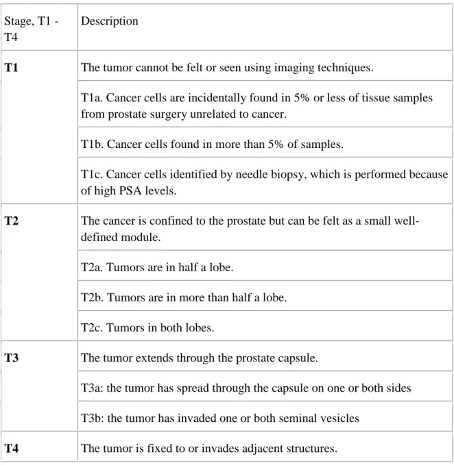
Additionally, the tumor size is regarded as a possible risk factor of prostate cancer. Studies have shown that an increase in tumor size led to an exponential increase in malignant tumors (Chan, 2012). Indeed, tumor cell has a relation with the risk of mortality amongst prostate cancer patients who are on observation (Andreas Josefsson, 2012). After the diagnosis of cancer, tumor stage checks the magnitude of severity as well as cancer spread. Table 1.1 describes four stages of tumor as T1 – T4, which represent the size as well as the spread of the tumor.

(19)

6

Table 1.1: Four stages of Tumor (University of Maryland). Stage, T1 -

T4

Description

T1 The tumor cannot be felt or seen using imaging techniques.

T1a. Cancer cells are incidentally found in 5% or less of tissue samples from prostate surgery unrelated to cancer.

T1b. Cancer cells found in more than 5% of samples.

T1c. Cancer cells identified by needle biopsy, which is performed because of high PSA levels.

T2 The cancer is confined to the prostate but can be felt as a small well-defined module.

T2a. Tumors are in half a lobe.

T2b. Tumors are in more than half a lobe. T2c. Tumors in both lobes.

T3 The tumor extends through the prostate capsule.

T3a: the tumor has spread through the capsule on one or both sides T3b: the tumor has invaded one or both seminal vesicles

(20)

7

1.1.3 Treatment

Prostate cancer in men may be treated using a variety of techniques such as bisphosphonate therapy, chemotherapy, hormone therapy, radiation therapy as well as surgery. The aforementioned techniques are utilized separately; however, in certain instances they can be integrated.

The most commonly used technique for treating cancer that has not spread beyond the gland is called surgery. A radical prostatectomy (RP) refers to a surgical process, which entails the removal of prostate gland alongside the attached seminal vesicles. During this procedure, the lymph nodes that are adjacent to the prostrate may be removed simultaneously. Radical prostatectomy (RP) is a common alternative for treating prostate cancer that has not spread to other areas of the body. Specifically, it is preferred when the patients are younger than 70 years, otherwise radiation therapy is preferred (Stangelberger, 2008). The follow up after the RP can detect the PSA level, which identifies the patients with elevated risk of local treatment failure or metastatic disease. Though PSA level after surgery is high in some cases, patients are still free of symptoms for extended periods of time. Therefore, the PSA level may not be enough to initiate additional treatment (National Cancer Institute).

1.2 Survival Analysis

Since cancer ranks as the second leading cause of death in the world, survival analysis techniques have been used to measure the risk, hazards, and average survival time for cancer patients. The common research involving cancer is based on time called the survival time. The term ‘survival time’ is used in reference to the number of days, weeks and years from the time patient’s observance begins until death takes place. Since 1950s, survival analysis has proved to be an important technique (Langova, 2008). There are several areas where survival analysis is applied which include demography, economics, engineering, epidemiology, health, medicine and biology. Additionally, there has been an increase in the use of survival analysis in areas of biostatistics as well as pharmaceuticals. There are several objectives for survival analysis which include estimation as well as interpretation of survivor function using survival data, comparison of survivor functions coupled with assessment of the link involving defined variables and time of survival (Langova, 2008). Since the survival analysis was provided with cancer data, we need

(21)

8

special data that is called clinical trials. They are conducted to determine the effectiveness of new treatment (Singh, and Mukhopadhyay, 2011). Usually in survival studies, the patients are kept over a long period of time, so other factors are important to be still continual over the period. The dependent variable within the survival analysis is composed of two attributes namely, time-to-event as well as event status. An endpoint occurs either when the event occurs or when the follow-up time has ended. There are several endpoints that can be the events such as death, relapse of disease, recurrence of a tumor, recovery or any designated experience of interest as shown in Table 1.2. It marks the indicator variable as 1 if the event of interest was observed or 0 if it was censored.

Table 1.2: The survival times

Starting Point End Point

Surgery Death/ Relapse/ Recurrence. Diagnosis Death/ Relapse/ Recurrence. Treatment Death/ Relapse/ Recurrence.

Standard statistical methods may not be used widely because the inherent distribution is abnormal and there is censoring of data (Bewick, 2004). Censoring of survival time occurs when the time of follow-up is available though it might have taken place unnoticed or has not taken place. Several techniques utilized in survival analysis include non-parametric, semi-parametric as well as parametric. Within the techniques two kinds of information involving clinical trial for survival analysis exist namely, censored as well as uncensored data. Exact data (uncensored data) refers to a situation whereby the participant is aware until the occurrence of event-of-interest.

(22)

9

1.2.1 Censored data

Censored data emerges as a critical issue for consideration in survival analysis, because it helps to indicate the kind of missing information. Censored data arises when a negative event takes place for instance, withdrawal of participant, difficulties in tracking the participant, participant has not encountered the suitable results or the relevant data is unavailable. Notably, an indicative variable with value 1 is used when the uncensored survival time has been identified and value of 0 is used for right-censored times (Zhao, 2008). Three separate scenarios involving censored data that rely on the follow-up times are in existence. However, this relies largely on the stage-level as well as risk-level for the patient.

1. Right censored refers to a patient who may not encounter a time failure for the event-of-interest until the follow-up duration elapses or withdraws from the study before it ends. 2. Left censored refers to a situation whereby the event-under-interest takes place prior to

enrolment. This scenario is not common.

3. Interval censored this situation takes place when an event-under-interest has a tendency of occurring in a specific time (Zhao, 2008).

(23)

10

Figure1.1: Illustration of left, right and interval censoring

The crosses in Figure 1.1 indicate when the failure occurs, while the arrows perpendicular to the time axis show the actual times (Aaserud, 2011).

Overall, the feature of censoring implies that special techniques of analyzing are essential. Most widely used technique for analyzing is right censored.

1.2.2 Functions related to survival analysis

Before choosing a technique for use in survival analysis, it is imperative that two functions, which are time dependent, are considered. They include survival function and hazard function that may be explained using the survival information.

(24)

11

 The survival function S(t) produces the survival probability approximately to time t. The survival function is essential for survival analysis. The Kaplan-Meier curve provides the survival function.

𝑆(𝑡) =𝑃(𝑇> 𝑡) = 1− 𝐹(𝑡),𝑡 ≥ 0. (Fox, 2002)

T represents a positive random variable that covers the time from commencement of the observation up to survival. 𝐹(𝑡) is the distribution function.

 The hazard function h(t) represents the probability condition of death at time t after survival time.

ℎ(𝑡) = lim_𝑑𝑑→0𝑃(𝑡 ≤ 𝑇< 𝑡_𝑑𝑡+𝑑𝑡|𝑇 ≥ 𝑡) ,𝑡 ≥0. A relationship between S(t) and h(t) is shown in the formula below:

ℎ(𝑡) =𝑓(𝑡)_{𝑆(𝑡) =}−𝑑log_𝑑𝑡𝑆(𝑡)

𝑓(𝑡) is the density function which gives the fraction of the original group for whom the event occurs during the time interval at t adjusted for the width of the time interval.

If one of 𝑆(𝑡) or ℎ(𝑡) is known, the other can be calculated.

𝑆(𝑡) = exp�− � ℎ(𝑢)𝑑𝑢𝑑

0 �= exp�−𝐻(𝑡)�,𝑡 ≥0.

Where 𝐻(𝑡) is the cumulative hazard function. 𝐻(𝑡) is difficult to interpret, but there is an easier way to make a clear interpretation. The way is to think of 𝐻(𝑡) as the cumulative force of mortality or if the event were a repeatable process, the number of events expected for each individual by time 𝑡.

(25)

12

𝑓(𝑡) =ℎ(𝑡) exp�− � ℎ(𝑢)𝑑𝑢𝑑

0 �,𝑡 ≥0.

Hazard ratio (HR)

It is expressed as the relative risk that is used to estimate the ratio of the hazard rate. In addition, it has been utilized for describing the outcome of the trials therapy in order to figure out the range the treatment can shorten the duration of the disease (Singh, and Mukhopadhyay, 2011).

The processing of statistical data should entail application of relevant techniques. The survival module is characterized by four essential techniques to fit survival models. These models are illustrated in Table 1.2. The last strategy in Table 1.2 that is more direct is the parametric technique (accelerated failure time), whereby there is assumption on the specified functional form of the baseline hazard (𝑡). Within this technique several distributions which acquire a central point are in existence such as Weibull, generalized gamma, log-logistic and lognormal. The aforementioned approaches are explained in chapter 3 and can be integrated into our information to ascertain their suitability.

Different models can be classified as: proportional hazards model (exponential and Weibull) and

proportional odds model (log-logistic). Figure 1.2 illustrates that the Weibull and exponential models can be both the accelerated failure time (AFT) model and proportional hazards model. In addition, it provides the commonly used parametric models.

(26)

13

Table 1.2: The main models for survival analysis

Technique Goal

Kaplan-Meier Estimate the probability of an individual surviving for a given time period

Log-rank Test Compare survival of two different groups of individuals.

Cox regression Detect clinical/ genomic/ epidemiologic variables, which contribute to the risk. Accelerated failure time (AFT) Used as an alternative model to the Cox

model where the proportional hazard assumption is not held constant.

Figure 1.2: Parametric models in survival analysis (Sewalem, 2012).

The above methods have different properties and interpretations. However, each model can summarize survival data.

(27)

14

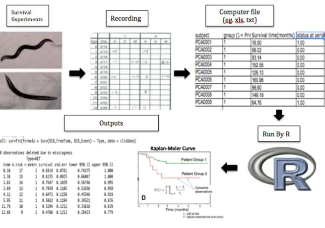
The steps of the survival analysis using R programming are shown in Figure 1.3 (Yang et al., 2011).

(28)

15

1.3 Objectives

There are some essential goals that are presented in the current study in order to clearly understand the important meaning of the survival analysis and how it deals with prostate cancer data.

1. The objective of the present study is to address some important questions related to prostate cancer survivorship for patients with primary or metastatic tumor. It is commonly understood that the risk of developing prostate cancer is higher in metastatic tumor than the primary. The objective of this thesis is to examine the efficiency of several methods that are commonly used to estimate survival functions in the presence of censored data. Kaplan-Meier analysis was performed to estimate survival in univariate analysis. We compare different techniques to estimate survival functions.

2. This research investigates the influence of standard clinical prognostic features on the survival time of prostate cancer patients. Particularly it seeks independent variable patterns to determine the survival times and identify the correlations among the variables of interest. For this goal the Cox model performed well, which identified covariates associated with survival.

The rest of the thesis is organized as follows:

Chapter 2 provides a literature review on survival analysis for cancer dataset. Chapter 3 presents the data set and its description to clearly understand it. Additionally, it provides in detail the methodology that was performed for survival analysis suitable for the given data. Chapter 4 summarizes and discusses the results. Chapter 5 concludes the study. Finally, appendices summarize R code and a few outcomes.

(29)

16

Chapter 2 Literature Review 2.1 Survival Analysis Study

Litwin, et al., (2000) faced significant challenges that kept them from bringing data together from different studies in order to assess disparities in results of treatment in various institutions. Initially, they were presented with different endpoints from the studies. Following this, they noticed that the different studies showed varying disease severity. Finally, usefulness of the results was limited by the differences in the techniques used to measure patient-focused outcomes. There are several clinical trials where survival analysis model was used. We present here some of the techniques of survival analysis for cancer data especially prostate and breast. Vinh-Hung, V. et al. (2002), Post-surgery radiation in early breast cancer: survival analysis of registry data

Vinh-Hung et al (2002) showed the survival advantage in patients diagnosed with early breast cancer, treated with post-surgery radiation. The current study tries to prolong these results through an organized population data analysis. This study made use of Epidemiology, Surveillance, and End Results (SEER) data on 83,776 women suffering from breast cancer diagnosed between 1988 and 1997, stage T1–T2, node positive or node negative. The proportional hazard models were used for the analysis.

Results showed that the best rates of survival were found with combined radiation and breast-conserving surgery in all cases. The available data indicate that post-surgery radiation provides a survival advantage irrespective of the type of surgery in node positive patients. Likewise, survival advantage was observed with post-surgery radiation and breast-conserving procedure in node negative patients.

Ray, M.E. et al. (2009), Potential surrogate endpoints for prostate cancer survival: analysis of a phase III randomized trial

In their study, Ray, M. E. et al. (2009) determined that surrogate endpoints for prostate cancer specific survival may reduce the length of the clinical trials for a patient’s prostate cancer. This

(30)

17

study assessed distant metastasis and failure of general medical treatment as possible substitutes for prostate cancer-specific survival using data from the Radiation Therapy and Oncology Group 92-02 randomized experiment.

They use data where patients (n = 1554 assigned randomly and 1521 evaluable for the study) having locally advanced prostate cancer had undergone 4 months with neoadjuvant and simultaneous androgen deprivation therapy with external treatment of beam radiation. These patients were then randomly assigned to either no additional treatment (control arm) or 24 extra months of androgen deprivation therapy (experimental arm). Statistics coming from the point of origin of examinations at three and five years for failure of general clinical treatment (meaning the recorded progression of local disease, distant or regional metastasis, induction of androgen deprivation therapy, or a prostate-specific antigen level of 25 ng/mL or more following radiation therapy) and/or distant metastasis were examined as substitute final stages for prostate cancer-specific survival at 10 years using Prentice's four criteria. The Cox proportional hazard (PH) models were utilized to provide the hazard ratio (HR) between the treatments. All statistical investigations were two-sided.

At 3 years, 1364 patients were surviving and provided data for evaluation. Both general clinical treatment failure and distant metastasis at 3 years indicated consistency with all four of Prentice's criteria for being a substitute for final stages for prostate cancer-specific survival at 10 years. At 5 years, 1178 patients were surviving and offered more data for evaluation. Even if prostate cancer-specific survival did not statistically vary substantially between arms of treatment at 5 years (P = .08), both final stages showed consistency with the remaining Prentice's criteria. They concluded that general clinical treatment failure and distant metastasis at 3 years may be possible with alternative endpoints for prostate cancer-specific survival at 10 years. However, these final stages must be verified with other collections of data.

Chan, Y.M. (2013), Statistical Analysis and Modeling of Prostate Cancer

The study performed by Chan (2013) provided a comparison of survival between African American and White men at the four distinct stages of prostate cancer under the same treatment. Moreover, the study made it possible to estimate the average difference in survival between

(31)

18

White and African American males diagnosed with prostate cancer and addressed some of the critical issues related to treatment.

There is a common perception that African American men have a greater risk of developing prostate cancer than men of other races. Nevertheless, with the use of parametric analysis, Chan’s study showed that the perception is more of a myth than reality. The study further recognized the presence of racial/ethnic differences by relating the average size of tumors, the median time of survival time, and the survival function between African American and White men. These outcomes emphasize the need for acknowledging the role that racial background plays in improving clinical targeting, and in so doing, advancing clinical results. Moreover, parametric survival analysis was conducted to approximate the survival rate of white men going through various treatments at every stage of prostate cancer. In addition, to comprehend the risk factors (tumor size, age, age and tumor size interaction) linked with survival time, a framework of accelerated failure time was created. The model could precisely forecast the survival rates of white men at each stage of prostate cancer according to the received treatment.

Lastly, the outcomes of parametric survival analysis and the framework of accelerated failure time model are compared among white men going through the same treatment at each disease stage.

Pulte, D. (2012), Changes in survival by ethnicity of patients with cancer between 1992–1996 and 2002–2006: is the discrepancy decreasing?

The study organized by Pulte et al (2012) emphasized that those patients of marginal race or ethnicity report lower rates of survival in most of cancer diagnosis cases. Over time, there exists few data regarding changes in the differences. Here, they evaluated changes in survival rates of patients with common cancers in two latest periods of time by ethnicity or race.

In their methods they utilized a structured period analysis to define relative survival (RS) for African–American (AA), non-Hispanic white (nHw), and Hispanic patients in the Epidemiology, Surveillance, and End Results database detected with usual solid and hematological distortions. The results show the RS for five years became better for nHw for every tumor detected, between +2% points (pancreatic cancer) to +16.4% points [non-Hodgkin's lymphoma, (NHL)]. Greater

(32)

19

progress was seen for Hispanics and AA than nHw in NHL, and prostate and breast cancer. There was less improvement for Hispanics and AA than for nHw for pancreatic and lung cancer. Statistically, for Hispanics and AA with acute leukemia or myeloma, no substantial improvement was observed. Disparities in survival remained between AA and Hispanics from 0.5% points for myeloma to 13.1% points for breast cancer

They conclude that there has been advancement in reducing the differences in survival between minorities and nHw in NHL, prostate and breast cancer. Minimal improvement has been possible in decreasing the differences for their cancers.

(33)

20

Chapter 3

Materials and Methodology 3.1 The Data source

Prostate survival data was obtained and generated from the Memorial Sloan Kettering Cancer Center (MSKCC). At MSKCC, each sample had been collected from the recipients of radical prostatectomy treatment. Out of the sample group, 181 patients were diagnosed with primary tumors along with one patient who has both metastases and primary tumor and 37 with metastases including the aforementioned patient. The association between survival, the tumor type, and the raw data contains 230 cases (rows) and 164 variables (columns). Additionally, for this recent analysis 40 variables have been chosen to improve the results. Detailed description of the data set can be found in the article written by Taylor et al. (2010). The format of the dataset is shown in Table 3.1, where they defined the data such as the type of tumor (primary or metastatic), age (years), race (White Non-Hispanic, Black Non-Hispanic, White Hispanic, and Black Hispanic) and so on. The data was converted from a factor into numeric, in order to apply it in R.

The data collected from MSKCC has some primary criteria to select patients after the radical prostatectomy (RP) treatment:

• Serum PSA testing every 3 months for the first year, 6 months for the second year, and annually thereafter. For all analyses described here, biochemical recurrence (BCR) was defined as PSA ≥ 0.2 ng/ml on two occasions.

• Following radical prostatectomy, patients were followed-up with history, and physical exam.

• The size of the primary tumor was known • Initial biopsy Gleason score is between 6 to 9.

• At the time of data analysis, patient follow-up was completed through December 2008. The age was between 37.3 and 83.

(34)

21

Table 3.1: Clinical trial data of prostate cancer.

Sample ID Type MetSite Race PreDxBxPSA DxAge BxGG1 …. PCA0171 PRIMARY NA White Non-Hispanic 8.20 60.87 3.00 …. PCA0172 PRIMARY NA White Non-Hispanic 17.20 52.00 4.00 …. PCA0173 PRIMARY NA White Non-Hispanic 5.24 66.16 3.00 …. PCA0174 PRIMARY NA White Non-Hispanic 4.60 54.32 4.00 …. PCA0175 PRIMARY NA Black Non-Hispanic 5.60 51.00 3.00 …. PCA0176 PRIMARY NA Black Non-Hispanic 8.10 53.55 3.00 …. PCA0177 PRIMARY NA White Non-Hispanic 5.63 59.78 4.00 …. PCA0178 PRIMARY NA White Non-Hispanic 4.60 61.83 3.00 …. PCA0179 PRIMARY NA White Non-Hispanic 40.24 64.89 4.00 …. PCA0180 PRIMARY NA White Non-Hispanic 8.03 67.17 4.00 …. PCA0181 PRIMARY NA White Non-Hispanic 27.00 69.01 4.00 …. PCA0182 MET Node White Hispanic 30.00 58.00 4.00 …. PCA0183 MET Bone White Non-Hispanic 182.10 82.00 5.00 …. PCA0184 MET Node White Non-Hispanic 27.00 69.00 3.00 …. PCA0185 MET Node White Non-Hispanic 27.00 69.00 3.00 ….

…. …. …. …. …. …. …. ….

The headings found in Table 3.1 are described in detail using proper medical language in Figure 3.1.

(35)

22

(36)

23

Descriptive statistics can provide some information about the distributions of the variables such as the average, minimum and maximum time in days for the censored and failed observations. In our data the descriptive statistics provided information for the two types of tumors: primary and metastatic as shown in Table 3.2. Patients in our study ranged in age from 37.3 to 83 years. An example of these statistics can be found in the following table. As the table shows, the PSA value was tested at less than 4, between 4 and 10, and greater than 10 ng/ml. There are 31 (17.2%) patients with primary tumors whose PSA was less than 4, and 4 patients of metastatic (12.5%). There are 105 (58.3%) patients with primary tumors whose PSA was between 4 and 10, and 6 (18.75%) patients of metastatic. Finally, there are 44 (24.5%) patients with primary tumors whose PSA was greater than 10, and 22 (68.75%) patients with metastatic.

(37)

24

Table 3.2: Descriptive statistics for the distributions of the variables (Taylor et al., 2010).

Characteristic Primary tumor Metastatic Age Median 58.3 60 Mean 58.3 60 Standard deviation 7 8.6 Min-max 37.3–83 41–82 PSA at diagnosis (ng/ml)

Median 6 (IQR 4.4, 9) 17 (IQR 8.6, 46.6) <4 31 (17.2%) 4 (12.5%) 4–10 105 (58.3%) 6 (18.75%) >10 44 (24.5%) 22 (68.75%) Initial biopsy Gleason score 5 2 (1%) -- 6 101 (56%) 2 (6%) 7 61 (34%) 16 (46%) 8 11 (6%) 8 (23%) 9 6 (3%) 9 (25%) Initial clinical stage cT1c 95 (52.4%) 8 (22%) cT2 76 (42%) 12 (33%) cT3 9 (5%) 3 (8%) cT4 -- 1 (3%) Not available -- 9 (25%)

(38)

25

3.2 Methodology

We examine non-parametric, semi-parametric and parametric methods to estimate the survival function for the given data.

3.2.1 Non-parametric Methods Kaplan Meier Estimates (K-M)

The first point to consider is how censoring can be adjusted in the K-M method in order to estimate the survival function. As the K-M method makes no assumption about the shape of the underlying survival curve, it is categorized as a non-parametric method for estimating a survival function. However, using a non-parametric analysis typically generated much wider confidence bounds than those calculated via parametric analysis. Parametric analysis shows how predictions outside the range of observations are not possible with non-parametric analysis.

As we have defined earlier in chapter 1, the survival function is the mathematical equation that describes a smooth curve, depicting the lifetime of the population of interest. When the survival time differs especially when some subjects are excluded in the study, K-M curve is one of the most common curves to tackle the likewise circumstances.

The characterization of all the subjects of the survival analysis by K-M method can use only three variables (Rich, et al., 2010). The first variable is the serial time which begins with the commencement of the treatment and gets censored from the study when it reaches the end point. At the end of the serial time, the second variable consists of the patient’s status. The third variable is the study groups the patients belong to.

The idea of this method is based on the probability of the surviving in k or more periods in the study and is a product of k probabilities when each period is observed under it. It is written by the following expression:

(39)

26

In the above equation 𝑝₁ constitutes surviving proportion in the first period, 𝑝₂ is the proportion survived over the second period, and so on. The equation below gives the proportion of surviving for period 𝑖 where they survived up to period 𝑖:

𝑝𝑖 = 𝑟𝑖 − 𝑑_𝑟 𝑖 𝑖 Where,

𝑟𝑖 is the number of patients living at start of the period 𝑖, and 𝑑𝑖 is the number of deaths.

Considerations in the K-M curves:

Identifications have to be made in the analysis of the K-M curve regarding the units of measurement according to the axes and the events of interest. After that, the evaluation of the curve, the number of the censored subjects and their distribution are very important. The number of participating subjects is much more if the curve consists of many small steps. However, limited number of participating subjects results in a curve with large steps. The time period of being alive of those patients who have been treated is measured in many medical studies.

In current study survival package of R program was used for survival analysis. In our data the first variable to characterize each subject of K-M survival analysis is the serial time in the column BCR_FreeTime, which is time until death (in months). The second variable status is given by column BCR_Event, its event (after RP as defined by rise of PSA level). The time to event (death) was estimated for a group of individuals. The third variable study group is the type of prostate cancer (primary or met). The instruction in R to estimate the survival function is given by:

(40)

27

The results sorted by ascending serial times beginning with the shortest times for each group are shown in Chapter 4. A subset of the data is used to look at primary tumors only according to the tumor Gleason score to show the estimate the survival time and to show which tumor grade has a higher rate.

The median is chosen for a summary measure as the distribution of survival time is positively skewed. Therefore, the median survival time is defined as 50% of the individuals under study expected to survive in their time.

Log Rank

The K-M survival curves can provide us an idea about the difference between survival functions among two or more groups. However, it cannot give us whether this observed difference is statistically significant. Hence, many methods can be utilized to test the equality of the survival functions for different groups. The log-rank is one commonly used non-parametric test for comparing two or more survival distributions of the patients; it is also called Mantel log-rank. Additionally, this method is useful when the risk of an event is always greater for one group than another in order to detect a difference between groups.

The steps to complete this method start with arranging the survival time for both censored and observed times. The log rank test is a form of Chi-square test distribution with one degree of freedom (Singh, and Mukhopadhyay, 2011) that calculates a test statistic used for testing a null hypothesis. In our study the log rank test was used to test the null hypothesis that the survival curves for all groups are the same. To clarify, it was used to test whether or not there is a difference between the populations in the probability of an event (here death) at any point in time. For each point of time the observed number of deaths in each group and the number of expected deaths are calculated to determine if there was a difference. The number of expected deaths is determined by multiplying the total number of events at a given point in time with the proportion of subjects who are at risk at that point (Dakhil, et al., 2012).

(41)

28 The calculation of the test is:

𝑋2_{(𝑙𝑙𝑙𝑙 𝑟𝑟𝑙𝑘) =}(𝑂1−𝐸1)2 𝐸1 +

(𝑂2−𝐸2)2

𝐸2 (Bewick, et al., 2004)

Here, 𝑂₁and 𝑂₂stand for the number of total events that have been observed within the groups of 1 and 2 respectively.

The expected number of events is represented by 𝐸₁ and𝐸₂.

The survdiff function in R implements the log rank test. In our study, this method is useful to detect the difference between two groups of tumor - primary and metastasis.

logDiff <- survdiff(Surv(BCR_FreeTime, BCR_Event) ~ Type, data = clinData)

3.2.2 Semi-parametric Methods Cox proportional hazard

The non-parametric methods are not useful for controlling the covariates and it requires categorical predictors. Therefore, the multivariate approaches are used when we have several prognostic variables. The most widely applicable and broadly implemented multivariate method in the survival analysis is the regression model of the Cox proportional hazards. In the year 1972 Cox showed the first light to the Cox model (Fox, 2002). The explanatory variables (determining the features of the patients with the estimation of the number of covariates and risk of death) and the response variables are combined. As any form can be adopted by the disturbance of the baseline, the nature of the model is semi-parametric (Fox, 2002). Disturbances are defined as the hurdles of death and the moments risked by death, which have been outlasted by the patients within a given period of time. There can be a number of homogenous regression models of Cox but hazard function is the variable to depend upon. However, the time factor does not affect the hazard function as it does in the survival function.

The Cox model, a regression method for survival data, provides an estimate of the hazard ratio which is always non-negative and its confidence interval. The hazard ratio is an estimate of the ratio of the hazard rate based on comparison of event rates. The hazard rate is the probability that if the event in question has not already occurred, it will occur in the next time interval, divided by

(42)

29

the length of that interval. The time interval is made very short, so that in effect the hazard rate represents an instantaneous rate. An assumption of proportional hazards regression is that the hazard ratio is constant over time.

The mathematical equation of the Cox model is:

ℎ(𝑡) = exp{ ℎ0 (𝑡) +𝑏1𝑥1+𝑏 2𝑥2+⋯+ 𝑏 𝑝𝑥𝑝}

Or logℎ(𝑡) = ℎ₀ (𝑡) + 𝑏₁𝑥₁+𝑏 ₂𝑥₂+⋯+ 𝑏 _𝑝𝑥_𝑝 (Fox John, 2002) Here,

h(t) represents the hazard function within the limited time period of t. The covariates of x1, x2, …., xp are also the explanatory variables.

If each explanatory variable xi is zero (exp ℎ₀ (𝑡)=1) then the hazard of the baseline is represented by ℎ₀(t). If covariates (risk factors) is characterized by dichotomy and is coded 1 if present and 0 if absent, respectively.

According to the implication of the proportionality, the quantities exp(bi) are known as the ratios of hazards. The interpretation of the quantity exp(bi) is an event when relative risks are evolved immediately irrespective of time . The individuals with the risk factors and individuals without the risk factors work equally with all the covariates. If the covariates are presupposed to be continuous then the interpretation of the quantity exp(bi) is an event where the risk factors are evolved immediately irrespective of time where the value of the covariate increased by 1 was compared with another individual provided the effects of all the individuals on the covariates are same. Binary and continuous are the two types of covariates. The h (t)/ ℎ₀ (𝑡) is known the hazard ratio.

The statistic package that triggers the changes in the hazards that are anticipated, helps to estimate the coefficients 𝑏₁, 𝑏 ₂… 𝑏 _𝑝. Since this method focuses on the relation, it is necessary for us to interpret the coefficients for each explanatory variable. The hazards will increase if the occurrence of the regression coefficient in explanatory variables is positive, and the hazards

(43)

30

decrease as an improved prognostic is yielded by the regression coefficient only when it is negative.

A Cox model was fitted by using an appropriate computer program in R to find the equation for the hazard as a function of several explanatory variables. This model was used to investigate the influence of standard clinical prognostic features on the survival time of Prostate cancer patients: Before we fit the Cox proportional hazard, the variables should be converted to numeric as

follows:

clinData $PathStage <- as.numeric(clinData $PathStage) clinData $PathGGS <- as.numeric(clinData $ PathGGS) clinData $ PathGG2 <- as.numeric(clinData $ PathGG2) The best fit model with four explanatory variables is given by:

coxFit2 <- coxph(formula = Surv(BCR_FreeTime, BCR_Event) ~ PreDxBxPSA + PathGGS + PathGG2 + PathStage, data = clinData)

The Adequacy of a model:

When clinical trials are performed, the primary analysis of the biomedical and biological applications has a number of available variables. However, the number of predictable errors can increase if the covariates are invalid (Liang and Guohua, 2008). The task of determining covariates for the statistical model has always been very sensitively critical in the process of data analysis. The selection of a proper model is broadly depended on the Akaike’s information criterion (AIC).

AIC is applied in order to choose one model from two competing ones having the possibilities of various ranges of parameters. The models mostly carry a great number of covariates that are feasible and due to this each parameter should be evaluated separately with dynamic scale in search of the most befitted model. AIC of lower amount in a model is the finest trigger in the betterment of a model (Symonds, et al., 2011).

The implementation of the proposed method is quite feasible in the concurrent software named R/Splus and others. The command used in R for this method is extractAIC.

(44)

31 The AIC will be:

𝐴𝐴𝐴 = −2𝐿𝐿+ 2(𝑐+𝑟) (Bradburn, et al., 2003) Here,

The logarithm of the similarities of the models is specified in LL.

c and a stand for the number of covariates and ancillary parameters respectively. Selection of covariates by step-wise selection using p-values:

For the creation of a preliminary model this is the best-suited approach and it is subject to change if its ability of befitting is good. To perform step wise p-value is measured to keep the variable or remove the variable from the model. The variable can be kept in the model when its associated significance level is less than this p-value. In contrast, if its associated significance level is greater than this p-value then the variable will be remove from the model.

Testing the proportional hazards assumption

The assumption of proportional hazards (PH) function is the finest techniques in the Cox model. This model help clarify the idea that multiplicative effect of each covariate in the hazards function is constant over time (Xue, et al., 2013). Quite often the assumption of PH is substantially important. The standard cohort studies offer a number of ways by which the assessment of the assumption of PH can be approached in addition to the statistical tests and graphical methods. “Conversely, graphical methods involve a moderate degree of subjectivity in interpretation. Statistical tests typically screen for the lack of fit of a Cox model.” ( Xue, et al., 2013).

Using Schoenfeld’s residuals

To monitor the capability of befitting of a statistical model is best judged by this useful method of residuals. The method to be presented here is the scaled residual method. The testing of time dependent covariates is the same as the test for a non-zero slope (both are equivalent) on the functioning time of the scaled Schoenfeld residuals in a linear regression. If the assumption of proportional hazard is violated then it is indicated by a non-zero slope.

(45)

32

In a Cox model each predictor variable defines the Schoenfeld residuals. Therefore, both the number of predictor variables and Schoenfeld residual variables are same. They are constructed on the assistance of each of the predictor variable to the log partial likelihood. The diagnosis of Cox regression models is greatly benefitted from the scaled Schoenfeld residuals, particularly in the assessment of the assumption of the proportional hazards (Grambsch and Therneau, 1994). Theoretically, the adjustments in the Schoenfeld residuals are incorporated according to the inverse of the covariance matrix of the Schoenfeld residuals. By using the slope of scaled Schoenfeld residuals against a function of time as our basis for the null hypothesis of the test on proportional hazards, it can apply the results to the generalized linear regression approach (Grambsch and Therneau, 1994).

The basis of the null hypothesis of the experiments in the proportional hazards is the scaled Schoenfeld residuals, which is the slope of the Schoenfeld residuals. This can be against a function of time which is zero for each predictor variables.

According to Schoenfeld the ith residual value can be plotted against 𝑡_𝑖 to verify the assumption that residuals are not affected by time. Partial residual is defined as the difference between the observed and expected value of 𝑋_𝑖 in the risk set 𝑅_𝑖. More precisely, the test statistic for an individual predictor variable is:

𝑟𝑖𝑘 =𝑋𝑖𝑘− 𝐸(𝑋𝑖𝑘|𝑅𝑖), (Fitrianto and Jiin, 2013)

In R program, the function of cox:zph calculates the assumption of the proportional-hazards with respect to covariates as it correlates the transforming time with the respective set of scaled Schoenfeld residuals. As a consequence, the proportional hazard assumption (PHA) does not need to be rejected provided the larger of p- value (>0.05) and its smaller p-value (<0.05) leads to the rejection of PHA.

In R the command is given as follows: Resplot <- cox.zph(coxFit2)

(46)

33

Cox- Snell

Cox- Snell residuals are used as their optimum distribution is achieved in the exponential form. As a result when different models with varied distribution are being worked upon, a common method can be applied to all of them. The possible drawback of this method lies in the nonparametric estimation of the baseline hazard function, which might violate the approximation exponentially of the Cox- Snell residuals.

It must be noted that use of Cox-Snell residuals for assessing the accuracy of survival models has not gained wide acceptance particularly when semi parametric Cox- models are used.

The following equation defines the model as:

𝑟𝑖 = 𝐻��𝑇0 𝑗�exp(𝛽 � 𝑋̀ 𝚤) ,𝑖= 1, 2, … ,𝑙 where

𝑟𝑖denotes a censored sample from a unit exponential distribution presuming that the applied Cox model will hold true.

𝐻�0 stands for values that lie near the actual value of H0. 𝛽 �̀ denotes values that lie near the actual value of 𝛽.

Plotting the log cumulative hazard plot of Cox-Snell residual with its best fitted straight line in R: Htilde <- cumsum(coxph.res2$n.event / coxph.res2$n.risk)

plot((coxph.res2$time), (Htilde), type = 's', col = 'blue') abline(0, 1, col = 'red', lty = 2)

Martingale residual

This residual is mainly used to assess how well a Cox model fits a series of observations. The martingale residual can actually quantify and produce a variable that will denote the interrelationship between a continuous predictor and the survival expectation for individuals. This model is examined as the best functional form for the given covariates.

(47)

34

The graph can be interpreted easily by superimposing a smoothed curve. There are many of smoother curves that can fit to scatterplot. One of the common algorithm used is LOESS or LOWESS smooth which is implemented in R package. To calculate the correct functional form of the variable, a Cox model is chosen with excluding the variable and a graph is plotted between the LOESS smooth of the martingale residuals against some change in the parameters of the variable. If the change in the parameters is correct then the graph will show a linear distribution. The equation depicting this is given below:

𝑀�𝚤(𝑡) =𝑁𝑖 (𝑡)− � 𝑌𝑖 𝑑 0 (𝑠)𝑒

𝛽̀�𝑋𝚤̀(𝑠)𝑑𝐻�₀(𝑠)

Where:

𝑀�is an acronym for 𝚤 𝑀�𝚤(∞). The residual is defined at each t, as the

𝑁𝑖 (𝑡) stands for the number of observed events over a time period t and includes the 𝑖𝑡ℎ subject. 𝑌𝑖 is a 0-1 process determining if the 𝑖𝑡ℎ subject is a risk at time t.

𝛽 �̀ which estimate by maximum partial likelihood estimator 𝛽 𝑒𝛽̀�𝑋̀𝚤_{is expected value for events for each}𝑖𝑡ℎ_subject

𝐻�0 denotes cumulative baseline hazard.

At times it is difficult to understand the graphs of martingale residuals as they have a skewed distribution and can have values ranging from (-∞, 1). This is the reason why deviance residuals are considered a better option for assessing model accuracy and pinpointing outliers.

The plot of martingale residual can be done for each variable in R as follows: plot(clinData2$PreDxBxPSA, rr,xlab="PreDxBxPSA",ylab="Residual") lines(lowess(clinData2$PreDxBxPSA, rr,iter=0),lty=2)

(48)

35

Deviance residual

It has been used to work on improperly projected observations. It was introduced by Therneau et al (1990) as a solution to the disadvantages of the martingale residual.

The deviance residual has a more symmetrical distribution about zero and can be defined as: 𝑑𝑖 =𝑠𝑖𝑙𝑙(𝑀𝑖)[−2{𝑀𝑖+𝛿𝑖 log(𝛿𝑖− 𝑀𝑖)}]

1

2 (Fitrianto and Jiin, 2013) Where:

𝑀𝑖 denotes martingale residual, function sign (.) stands for the sign function. 𝛿𝑖 observed number of events for 𝑖𝑡ℎ observation with 1 or 0.

Observations that lie on the extremes of the deviance residual are those that are not in accordance with the model parameters and are designated as outliers. In case of minimum censoring approximately < 25% deviance residuals achieve a more symmetrical form as compared to martingale residual and the overall distribution is in a pattern that closely resembles normal distribution.

This is how we can get deviance residuals from R:

plot(coxFit2$linear.predictor, dev.res, xlab = 'Risk Score', ylab = 'Deviance residuals') abline(0,0,lty=2,col='red')

3.2.3 Parametric Methods

Accelerated Failure Time Model (AFT):

The type of this model is completely different and the survival time data is evaluated by it. It has been presupposed that the linear function of the covariates serves as the time logarithm. It has been assumed further that the scale of time would affect the change in the survival of the covariates. It has been represented as: