New Algorithms for Uncertainty Quantification and Nonlinear Estimation of Stochastic Dynamical Systems

A Dissertation by

PARIKSHIT DUTTA

Submitted to the Office of Graduate Studies of Texas A&M University

in partial fulfillment of the requirements for the degree of DOCTOR OF PHILOSOPHY

August 2011

A Dissertation by

PARIKSHIT DUTTA

Submitted to the Office of Graduate Studies of Texas A&M University

in partial fulfillment of the requirements for the degree of DOCTOR OF PHILOSOPHY

Approved by:

Chair of Committee, Raktim Bhattacharya Committee Members, Suman Chakravorty

John L. Junkins Aniruddha Datta Head of Department, Dimitris C. Lagoudas

August 2011

ABSTRACT

New Algorithms for Uncertainty Quantification and Nonlinear Estimation of Stochastic Dynamical Systems. (August 2011)

Parikshit Dutta, B.Tech.; M.Tech., Indian Institute of Technology, Kharagpur Chair of Advisory Committee: Dr. Raktim Bhattacharya

Recently there has been growing interest to characterize and reduce uncertainty in stochastic dynamical systems. This drive arises out of need to manage uncertainty in complex, high dimensional physical systems. Traditional techniques of uncertainty quantification (UQ) use local linearization of dynamics and assumes Gaussian prob-ability evolution. But several difficulties arise when these UQ models are applied to real world problems, which, generally are nonlinear in nature. Hence, to improve per-formance, robust algorithms, which can work efficiently in a nonlinear non-Gaussian setting are desired.

The main focus of this dissertation is to develop UQ algorithms for nonlinear systems, where uncertainty evolves in a non-Gaussian manner. The algorithms devel-oped are then applied to state estimation of real-world systems. The first part of the dissertation focuses on using polynomial chaos (PC) for uncertainty propagation, and then achieving the estimation task by the use of higher order moment updates and Bayes rule. The second part mainly deals with Frobenius-Perron (FP) operator the-ory, how it can be used to propagate uncertainty in dynamical systems, and then using it to estimate states by the use of Bayesian update. Finally, a method to represent the process noise in a stochastic dynamical system using a finite term Karhunen-Lo`eve (KL) expansion is proposed. The uncertainty in the resulting approximated system is propagated using FP operator.

The performance of the PC based estimation algorithms were compared with extended Kalman filter (EKF) and unscented Kalman filter (UKF), and the FP oper-ator based techniques were compared with particle filters, when applied to a duffing oscillator system and hypersonic reentry of a vehicle in the atmosphere of Mars. It was found that the accuracy of the PC based estimators is higher than EKF or UKF and the FP operator based estimators were computationally superior to the particle filtering algorithms.

ACKNOWLEDGMENTS

I would like to give special thanks to Dr. Raktim Bhattacharya who has been a mentor and a friend. His creativity and drive have been essential to the completion of this work. Secondly, I would like to thank Dr. Suman Chakravorty for his guidance during my time as graduate student and clarifying several important concepts. I would also like to thank Dr. John L. Junkins for inspiring me, and helping me build the fundamental understanding of estimation theory.

My appreciation also goes to all my friends who have been very supportive and have helped me to maintain my sanity while completing this work. I would especially like to thank Abhishek, Baljeet, Avinash and Ramesh with whom I have worked and shared several good times at the CISAR laboratory. Their support and inspiration were of immense help towards completion of my work. I would also like to thank several other friends for always being there to share both laughter and hardship.

Last, but not the least I would like to thank my family especially my parents for everything they have done for me, and my uncle who helped me develop my interest in science.

TABLE OF CONTENTS

CHAPTER Page

I INTRODUCTION. . . 1

A. Background . . . 1

B. Contribution of This Dissertation . . . 7

II SEQUENTIAL STATE ESTIMATION METHODS . . . 9

A. Sequential State Estimation for Linear Systems . . . 10

1. Kalman Filter . . . 11

2. Linear Non-Gaussian Filter . . . 12

B. Sequential State Estimation for Nonlinear Systems . . . 14

1. Extended Kalman Filter . . . 15

2. Unscented Kalman Filter . . . 16

3. Particle Filters . . . 20

a. Step 1: Initialization of the Filter . . . 21

b. Step 2: Propagation . . . 21

c. Step 3: Update . . . 22

d. Step 4: State Estimate . . . 22

e. Resampling . . . 23

4. Other Sequential Monte Carlo Methods . . . 24

C. A Simple Example . . . 25

D. Summary of the Chapter . . . 27

III POLYNOMIAL CHAOS . . . 31

A. Generalized Polynomial Chaos Theory . . . 31

1. Wiener-Askey Orthogonal Polynomials . . . 32

B. Approximation of the Solution of Ordinary Differential Equations with Uncertainty . . . 34

1. Getting the Moments of the States . . . 35

2. A Simple Example . . . 37

C. Nonlinear State Estimation Using Polynomial Chaos and Higher Order Moments Update . . . 39

1. Step 1: Initialization of State . . . 40

2. Step 2: Propagation of Uncertainty and Computa-tion of Prior Moments . . . 40

CHAPTER Page

3. Step 3: Update Phase . . . 41

4. Step 4: Estimation of Posterior Probability Distribution 44 5. Step 5: Generation of Basis Functions . . . 48

D. Nonlinear Estimation Using Polynomial Chaos and Up-date Using Bayesian Inference . . . 48

1. Step 1: Initialization of State and Propagation of Uncertainty . . . 49

2. Step 2: Calculating the Posterior Probability Den-sity Function . . . 49

3. Step 3: Getting the State Estimate . . . 50

4. Step 4: Regeneration of Basis Functions . . . 51

E. Application to Duffing Oscillator . . . 51

1. Results for Estimation with Higher Order Moments Update . . . 51

2. Results for Estimation Using Bayesian Inference . . . 56

F. Application to Hypersonic Reentry . . . 56

G. Limitations of Polynomial Chaos . . . 74

IV THE FROBENIUS-PERRON OPERATOR. . . 76

A. Analysis of Densities in State Space Using Frobenius-Perron Operator . . . 76

1. Discrete-Time Systems . . . 76

2. Continuous-Time Systems . . . 79

3. Properties of Frobenius-Perron Operator . . . 81

B. Method of Characteristics for Solving First Order Lin-ear Partial Differential Equations . . . 81

C. Uncertainty Propagation in Dynamical Systems Using FP Operator . . . 82

1. Accuracy in Prediction of Uncertainty . . . 85

D. Nonlinear Estimation Using Frobenius-Perron Operator . . 88

1. Step 1: Initialization Step . . . 88

2. Step 2: Propagation Step . . . 88

3. Step 3: Update Step . . . 89

4. Step 4: Getting the State Estimate . . . 89

5. Step 5: Resampling . . . 90

E. Application of Nonlinear Estimation Using FP Operator . 90 1. Application to a Duffing Oscillator System . . . 91

CHAPTER Page

a. Sensitivity Analysis . . . 104

3. Application to Six-State Vinh’s Equation . . . 108

F. Limitations of Using Frobenius-Perron Operator . . . 110

V THE KARHUNEN LO`EVE EXPANSION . . . 116

A. Stochastic Dynamical Systems . . . 116

1. Solution Methodology . . . 117

2. Uncertainty Propagation in Stochastic Dynamical Systems . . . 119

B. The Karhunen Lo`eve Expansion Applied to Stochastic Dynamical Systems . . . 120

1. KL Expansion of Wiener Process . . . 121

2. KL Expansion Applied to Langevin Equation . . . 122

C. Convergence of Solutions . . . 123

1. Verification of Convergence in Distribution . . . 123

2. Convergence in Mean Square Sense . . . 132

D. Karhunen Lo`eve Frobenius-Perron Formulation . . . 138

1. Illustrative Examples . . . 139

E. State Estimation Using Karhunen Lo`eve Expansion and Frobenius-Perron Operator . . . 140

1. State Estimation of Vanderpol’s Oscillator . . . 140

2. Application to Hypersonic Reentry . . . 142

F. Summary . . . 149

VI CONCLUSIONS AND SCOPE OF FUTURE WORK . . . 150

A. Future Work . . . 151

1. Stochastic Control . . . 151

2. Multiphysical Dynamical Systems . . . 152

3. Dimensional Scaling . . . 152 REFERENCES . . . 154 APPENDIX A . . . 171 APPENDIX B . . . 177 APPENDIX C . . . 182 VITA . . . 184

LIST OF TABLES

TABLE Page

I Algorithm for linear non-Gaussian filtering . . . 14 II Correspondence between choice of polynomials and given

distri-bution of ∆ (Xiu and Karniadakis, 2002) . . . 33 III Explanation and values of the constants for Martian atmosphere

(Sengupta and Bhattacharya, 2008) . . . 59 IV Scaling constants for base units . . . 60 V Normalization factors for measurements . . . 61 VI Computational time taken per filtering step for each estimation

algorithm. Listed times are in seconds . . . 100 VII Normalization factors used for measurements . . . 109 VIII Normalization factors used for measurements (six state Vinh’s

equation with noise) . . . 145 IX The first ten Hermite polynomials . . . 172

LIST OF FIGURES

FIGURE Page

1 Plot of estimation errors and ±3σ limits for a) EKF b) UKF c) particle filter for the system in Eqn. (2.27a) & Eqn. (2.27b). The

solid lines are estimation errors and the dashed lines are±3σ limits. 26 2 Plot of estimation errors and ±3σ limits for a) EKF b) UKF c)

particle filter for the system in Eqn. (2.27a) & Eqn. (2.27b). The measurement update interval is 0.3s. The solid lines are

estima-tion errors and the dashed lines are ±3σ limits. . . 28 3 Plot of square root of difference between evolving variance of each

state and CRLB. The solid line is EKF the starred line is UKF

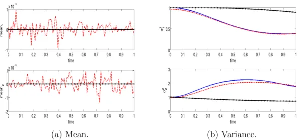
and the dashed line is particle filter. . . 29 4 Plots for a) mean b) variance of the Duffing oscillator in Eqn.

(3.10) & Eqn. (3.11) obtained from gPC scheme (solid) and Monte

Carlo (dashed) and linearized dynamics (star-solid) simulations. . . 39 5 Flowchart of polynomial chaos based estimation algorithms. . . 52 6 Evolution initial condition uncertainty for Duffing oscillator.

Prob-ability density functions were obtained using high fidelity Monte

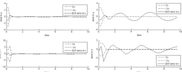
Carlo simulations. . . 53 7 Performance of EKF estimators. Dashed lines represent±3σ

lim-its and the solid line represents error in estimation. . . 54 8 Performance of gPC estimators. Dashed lines represent±3σ

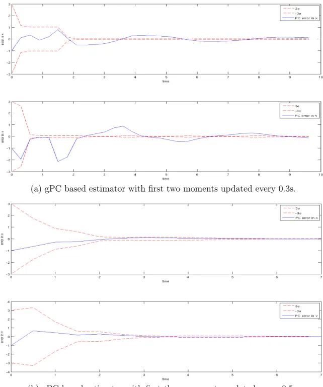
lim-its and the solid line represents error in estimation. . . 55 9 Plots for time (x-axis) vs. ±3σ limits (dashed lines) and

estima-tion error (solid lines) (y-axis) for gPC based estimators and EKF

FIGURE Page 10 (a) Mean and (b) standard deviation of the true system (solid) and

the approximated system (dashed) obtained from Monte Carlo

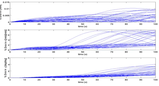
simulations. . . 63 11 Percentage error in states of the approximated system from true system. 64 12 Performance of (a) EKF and (b) UKF based estimator with true

initial states as [Rm + 61 km 2.42 km/s −8.91o]T and update interval of 20s. The dashed lines represent ±3σ limits and the

solid line represents error in estimation. . . 66 13 Performance of the gPC based estimator with true initial states

as [Rm+ 61 km 2.42 km/s −8.91o]T and update interval of 20s. The dashed lines represent±3σlimits and the solid line represents

error in estimation. . . 67 14 Performance of (a) EKF and (b) UKF based estimator with true

initial states as [Rm + 61 km 2.42 km/s −8.91o]T and update interval of 40s.The dashed lines represent±3σ limits and the solid

line represents error in estimation. . . 68 15 Performance of the gPC based estimator with true initial states

as [Rm+ 61 km 2.42 km/s −8.91o]T and update interval of 40s. The dashed lines represent±3σlimits and the solid line represents

error in estimation. . . 69 16 Performance of (a) EKF and (b) UKF based estimator with true

initial states as [Rm+ 61 km 2.64 km/s −8.1o]T and update in-terval of 20s. The dashed lines represent±3σ limits and the solid

line represents error in estimation. . . 71 17 Performance of the gPC based estimator with true initial states

as [Rm+ 61 km 2.64 km/s −8.1o]T and update interval of 20s. The dashed lines represent±3σlimits and the solid line represents

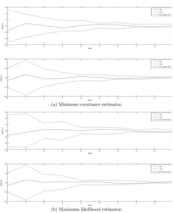
error in estimation. . . 72 18 Performance of (a) MCE, (b) MLE and (c) MEE criterion for state

estimates. The true initial states are [Rm + 61 km 2.42 km/s − 8.91o_]T _{and update interval is 20s. The dashed lines represent}

FIGURE Page 19 Long term statistics, up to 10 seconds predicted by Monte Carlo

(dashed line) and polynomial chaos (solid line) for the system in Eqn. (3.10) & Eqn. (3.11). The x-axis represents time and y-axes

are the states. . . 75 20 Method of characteristics. Number of samples = 500. System is

Duffing oscillator. The black circle shows the location and the PDF value (color coded) of an arbitrary sample point at different

time instances. . . 84 21 Comparison of FP and Monte Carlo based approximation of

den-sity functions. . . 86 22 Performance of the estimators with measurement update interval

as 0.3s. . . 92 23 Performance of the estimators with measurement update rate as 0.6s. 93 24 Generic particle filter. True initial states are [Rm+61 km 2.64 km/s−

8.1o_]T _{and update interval is 20s. The dashed lines represent±3σ}

limits and the solid line represents error in estimation. . . 95 25 Bootstrap filter. True initial states are [Rm+ 61 km 2.64 km/s −

8.1o]T and update interval is 20s. The dashed lines represent±3σ

limits and the solid line represents error in estimation. . . 95 26 Performance of the Frobenius-Perron estimator with true initial

states as [Rm + 61 km 2.64 km/s − 8.1o]T and update interval of 20s. The dashed lines represent ±3σ limits and the solid line

represents error in estimation. . . 96 27 Plots for √σ2 _{−CRLB vs. time. In the legend, ’BPF’, ’gPF’}

and ’FP’, represent bootstrap filter, generic particle filter and

Frobenius-Perron operator based estimator respectively. . . 96 28 Generic particle filter with 7000 particles. True initial states are

[Rm+ 61 km 2.64 km/s −8.1o]T and update interval is 20s. The dashed lines represent ±3σ limits and the solid line represents

FIGURE Page 29 Bootstrap filter with 7000 particles. True initial states are [Rm+

61 km 2.64 km/s −8.1o]T and update interval is 20s. The dashed lines represent ±3σ limits and the solid line represents error in

estimation. . . 97 30 Generic particle filter with 10000 particles. True initial states are

[Rm+ 61 km 2.64 km/s −8.1o]T and update interval is 20s. The dashed lines represent ±3σ limits and the solid line represents

error in estimation. . . 99 31 Bootstrap filter with 10000 particles. True initial states are [Rm+

61 km 2.64 km/s −8.1o_]T _{and update interval is 20s. The dashed} lines represent ±3σ limits and the solid line represents error in

estimation. . . 99 32 Percentage error in estimation with 7000 particles. True initial

states are [Rm + 61 km 2.64 km/s −8.1o]T and update interval is 20s. In the legend, ’BF’, ’gPF’ and ’FP’, represent bootstrap filter, generic particle filter and Frobenius-Perron operator based

estimator respectively. . . 100 33 Percentage error in estimation with number of particles for FP

based operator (FP), generic particle filter (gPF) and bootstrap filter (BF), 7000, 20000, and 25000 respectively. True initial states

are [Rm+ 61 km 2.64 km/s −8.1o]T and update interval is 20s. . . 101 34 Plots for 3rd and 4th order moments for particle filter with 100,000

particles- (dashed line) and FP operator based filter with 7000

samples- (solid line). . . 102 35 Plots for percentage error in 3rd and 4th order moments for

boot-strap filter (BF), generic particle filter (gPF) and FP operator based filter (FP), all with 7000 particles. Percentage deviation

taken from particle filter with 100,000 particles. . . 103 36 FP operator based filter with measurement noise 6×10−4I3 in

scaled units (number of samples = 7000). True initial states are [Rm+ 61 km 2.64 km/s −8.1o]T. The dashed lines represent±3σ

FIGURE Page 37 FP operator based filter measurement update interval is 40s

(num-ber of samples = 7000). True initial states are [Rm+61 km 2.64 km/s− 8.1o_]T _{. The dashed lines represent ±3σ limits and the solid line}

represents error in estimation. . . 105 38 Generic particle filter with measurement noise 6×10−4I3in scaled

units (number of samples = 25000) True initial states are [Rm+ 61 km 2.64 km/s −8.1o]T. The dashed lines represent±3σlimits

and the solid line represents error in estimation. . . 106 39 Generic particle filter measurement update interval is 40s (number

of samples = 25000). True initial states are [Rm+61 km 2.64 km/s− 8.1o_]T _{. The dashed lines represent ±3σ limits and the solid line}

represents error in estimation. . . 106 40 Bootstrap filter with measurement noise 6 × 10−4I3 in scaled

units (number of samples = 20000) True initial states are [Rm+ 61 km 2.64 km/s −8.1o_]T_{. The dashed lines represent±3σlimits}

and the solid line represents error in estimation. . . 107 41 Bootstrap filter measurement update interval is 40s (number of

samples = 20000). True initial states are [Rm+61 km 2.64 km/s− 8.1o_]T _{. The dashed lines represent ±3σ limits and the solid line}

represents error in estimation. . . 107 42 Performance of FP operator based filter with 9000 particles, when

applied to six state Vinh’s equation. The dashed lines represent

±3σ limits and the solid line represents error in estimation. . . 111 43 Performance of generic particle filter with 9000 particles, when

applied to six state Vinh’s equation. The dashed lines represent

±3σ limits and the solid line represents error in estimation. . . 112 44 Performance of the bootstrap filter with 9000 particles, when

ap-plied to six state Vinh’s equation. The dashed lines represent±3σ

limits and the solid line represents error in estimation. . . 113 45 Performance of generic particle filter with 30000 particles, when

applied to six state Vinh’s equation. The dashed lines represent

FIGURE Page 46 Performance of the bootstrap filter with 25000 particles, when

applied to six state Vinh’s equation. The dashed lines represent

±3σ limits and the solid line represents error in estimation. . . 115 47 Scatter plot of initial and the back-propagated elements for a given

sample. Blue circles are the original sample and the red ones are

the back-propagated sample. . . 128 48 Plot of empirical CDF of ˆy₀j and uniform CDF for a given sample. . . 129 49 Plot DM value for all the 100 samples. The samples above the

red and black lines fail when α= 0.05 and 0.01 respectively. . . 129 50 Plot DM value for all the 100 samples for a. N = 76 and b.

N = 91. The samples above the red and black lines fail when

α= 0.05 and 0.01 respectively. . . 130 51 Plot DM value for all the 100 samples for a. N = 21 and b.

N = 76, with increased M = 1000. The samples above the red

line fails whenα = 0.05. . . 131 52 Plot of empirical CDF of √M DM (red) and Kolmogorov CDF

(blue). . . 131 53 Plot of sup

x∈_R

|FMs(x)−FK(x)|vs. Ms . . . 132 54 Uncertainty propagation for Vanderpol’s oscillator Eqn. (5.40)

in top row of each figure, and Duffing oscillator Eqn. (5.41) in

bottom row of each figure. . . 141 55 ±3σ plots for a) KLFP-based estimator and b) Generic particle

filter. . . 143 56 Estimation errors (solid lines) and ±3σ limits (dashed lines) for

particle filter based estimator. . . 146 57 Estimation errors (solid lines) and ±3σ limits (dashed lines) for

FIGURE Page 58 Plot for univariate marginal density for particle filter (dashed line)

and KL expansion and FP operator based estimator (solid line).

Hereh=r−Rm and the y-axis denotes PDF value. . . 148 59 Plot for bivariate marginal density for particle filter (top row) and

KL expansion and FP operator based estimator (bottom row) for 4 state combinations. Here h =r−Rm. The PDF value is color

coded, red is high PDF and blue is low. . . 149 60 Locations of eigenvalues of the system in Eqn. (A.1), when Monte

Carlo approximation is used (red circles) and when PC

approxi-mated dynamics in Eqn. (A.3) is used (blue). . . 175 61 PDF of the eigenvalue distribution on the complex plane. Blue

represents low probability regions and red is high probability

re-gion. Eigenvalues represented in black. . . 176 62 Plots for estimation error and ±3σ limits for a) Kalman filter b)

FP operator based estimator c) particle filter. . . 179 63 Normalized Wasserstein distance between posterior PDFs of Kalman

filter and FP operator based estimator (solid line) and Kalman

filter and particle filter (dashed line). The value of R= 1/2. . . 180 64 Normalized Wasserstein distance between posterior PDFs of Kalman

filter and FP operator based estimator (solid line) and Kalman

filter and particle filter (dashed line). The value of R= 2. . . 181 65 Normalized Wasserstein distance between posterior PDFs of Kalman

filter and FP operator based estimator (solid line) and Kalman

CHAPTER I

INTRODUCTION A. Background

Uncertainty quantification in stochastic dynamical systems is a challenging field that has received attention for over a century. Understanding the impact of uncertainty in complex physical system has become a primary topic of research over the years. Problems due to uncertainty may arise in myriad areas of application ranging from robotics (e.g. path planning in an uncertain environment) and astrodynamics (eg. trajectory estimation of 99942 Aphophis) to structural engineering (e.g. excitation of a building caused by siesmic events) and petroleum engineering (eg. study of flow of oil through a reservoir with uncertain porosity). A large class of such problems deal with uncertainty in physical model and system parameters. Estimation of parame-ters in this scenario is typically a hard problem due to lack of frequent measurements and underlying nonlinearities in system dynamics. Thus the evolution of uncertainty, which can be non Gaussian, needs to be predicted over longer intervals of time. These issues undermine the validity of the classical linear Gaussian theory. Sequential es-timation algorithms, based on Monte Carlo (MC) simulations are most commonly used in such cases. However for systems having three or more dimensions, MC based techniques may be computationally expensive as ensemble size required to guarantee convergence, increases exponentially with number of states. Hence a nonlinear esti-mation algorithm, superior to the existing methods in terms of convergence of errors and computational complexity is desired.

Estimation of states and parameters for dynamical systems in general, are gen-The journal model is IEEE Transactions on Automatic Control.

erally performed in the Bayesian framework, where uncertainty is represented as probability density functions (PDF). For linear Gaussian systems, it is possible to get exact analytical expressions for evolving sequence of moments, which characterizes the PDF completely. This method is widely know as Kalman filter [1]. For nonlinear systems exhibiting Gaussian behavior, the system is linearized locally, about the cur-rent mean, and the covariance is propagated using the approximated linear dynamics. This method is used in extended Kalman filters (EKF) [2]. It is well known that this approach performs poorly when the nonlinearities are high, resulting in an unstable estimator [3, 4, 5, 6]. However, the error in mean and covariance can be reduced if the uncertainty is propagated, using the nonlinear dynamics, for a minimal set of sample points, called sigma points. The PDF of the states, characterized by sigma points, capture the posterior mean and covariance accurately to the third order (Taylor series expansion) for any nonlinearity with Gaussian behavior. This technique has resulted in the unscented Kalman filter (UKF) [7]. The aforementioned filters are based on the premise of Gaussian PDF evolution. If the sensor updates are frequent then EKF and UKF may yield satisfactory results. However, for nonlinear systems, if the sensor updates are slow, these filters result in inaccurate estimates [8].

Recently, simulation-based sequential filtering methods, using Monte Carlo sim-ulations, have been developed to tackle nonlinear system with non-Gaussian uncer-tainty [9, 10]. Monte Carlo methods involve representing the PDF of the states using a finite number of samples. The filtering task is obtained by recursively generat-ing properly weighted samples of the state variable usgenerat-ing importance samplgenerat-ing [11]. These filters, based on sequential MC methods are known as Monte Carlo filters [12]. Amongst them, the most widely used is the particle filter [13, 14, 15, 16]. Here en-semble members or particles are propagated using the nonlinear system dynamics. These particles with proper weights, determined from the measurements, are used

to obtain the state estimate. However, particle filters require a large number of en-sembles for convergence, leading to higher computational costs [17]. This problem is tackled through resampling [13, 18, 8]. Particle filters with resampling technique are commonly known as bootstrap filters [8]. It has been observed that bootstrap filters introduce other problems like loss of diversity amongst particles [15], if the resampling is not performed correctly. Recently developed techniques have combined importance sampling and Markov-Chain-Monte Carlo (MCMC) methods to generate samples to get better estimates of states and parameters [19]. Several other methods, like reg-ularized particle filter [20], and filters involving MCMC move step [21], have been developed to improve sample diversity. At the same time, even with resampling, due to the simulation based nature of these filters, the ensemble size scales exponentially with state dimension for large problems [22]. To circumvent this problem, particle filters based on Rao-Blackwellization have been developed to partially solve the esti-mation problem analytically [23]. However, its application is limited to systems where the required partition of the state space is possible. An excellent comparison of the various nonlinear filtering algorithms is available in ref. [24].

Nonlinear estimation algorithms based on polynomial chaos theory [25] and Frobenius-Perron operator [26] has been proposed in this work. Polynomial chaos (PC) is used to approximate any random process as linear combination of orthog-onal basis functions. The advantage of using PC is that an alternate deterministic dynamical system can be created from the stochastic system, which is then used to propagate uncertainty. Polynomial chaos was first introduced by Wiener [27] where Hermite polynomials were used to model stochastic processes with Gaussian random variables. According to Cameron and Martin [28], such an expansion converges in the L2 sense for any arbitrary stochastic process with finite second moment. This applies

to various continuous and discrete distributions using orthogonal polynomials from the so-called Askey-scheme [30] and demonstrated L2 convergence in the

correspond-ing Hilbert functional space. This is popularly known as the generalized polynomial chaos (gPC) framework. The gPC framework has been applied to various applications including stochastic fluid dynamics [31, 32], stochastic finite elements [25], and solid mechanics [33, 34]. In the context of nonlinear estimation, polynomial chaos has been applied by Blanchard et al. [35, 36], where uncertainty prediction was computed us-ing gPC theory for nonlinear dynamical systems, and estimation was performed usus-ing linear output equations and classical Kalman filtering theory. It has been shown that PC is computationally more efficient than Monte Carlo simulations [29]. Hence, it is expected that, the estimation algorithm presented here will be computationally more efficient than particle filters. However, such an analysis has not been performed, and is a subject of our future work. Here we have applied gPC theory to estimate states of a Duffing oscillator and hypersonic vehicle reentering Mars’ atmosphere.

The Frobenius-Perron operator determines the time evolution of probability den-sity function (PDF) through a system, and as shown later is computationally efficient than particle filters. The Frobenius-Perron operator has been used in the physics community to study evolution of uncertainty in dynamical systems [26]. In contin-uous time, the Frobenius-Perron operator is defined by the Liouville equation [37], which is the Fokker-Planck equation [38] without the diffusion term. It has been shown that the Frobenius-Perron operator or the Liouville equation, predicts evolu-tion of uncertainty in a more computaevolu-tionally efficient manner than Monte Carlo [39]. Based on this fact, we can expect a nonlinear filtering algorithm in this framework to be computationally more efficient than particle filters. However, it is important to note that the Frobenius-Perron operator only addresses parametric uncertainty. Use of Liouville equation to develop a nonlinear filtering algorithm was first presented

by Daum et al. [40], where the process of the filtering algorithm has been outlined. In this work we have applied Frobenius-Perron operator theory to a state estimation problem arising in hypersonic flights and perform a direct comparison with particle filters.

The above mentioned uncertainty propagation methods are applicable only when the dynamical system has initial state or parametric uncertainty. In presence of process noise, the evolution of densities are given by the Kramers-Moyal expansion [41]. This is a partial differential equation which characterize PDF propagation in any nonlinear system having process noise. A special case arises when we limit ourselves to additive Gaussian white noise as stochastic forcing. Then, the first two terms of the Kramers-Moyal expansion is sufficient to describe the evolving densities. This is referred to as the Fokker-Planck equation or Kolmogorov forward equation [42]. There are several methods, by which we can approximately determine the solution of the Fokker-Plank equation. A brief treatise of the most popular methods can be found in the book by Riskin [38]. Several methods which deal with numerical solutions of the Fokker-Planck equation have been developed over the years [43, 44, 45]. The numerical algorithms, intend to solve the Fokker-Planck equation using grid based methods like FEM, to evaluate the densities in a structured grid [46, 47, 48], or by using meshfree methods, by evaluating densities at randomly selected points to get the final PDF [49, 50]. Several researchers have used Monte Carlo based techniques to get an approximation of the solution of Fokker-Planck equation using finite number of samples [51, 50]. Another popular technique of solving Fokker-Planck equation involves approximating the PDF as linear combination of known functions. Researchers have often used known densities as the basis functions for approximation. This method is popularly known as kernel density estimation [52]. There are several techniques which solve the Fokker-Planck equation using this method [53, 54]. One

can also use known functions to get a finite dimensional approximation of the operator generated by the Fokker Planck equation. This method is useful as it converts the Fokker Planck partial differential equation into an approximate ordinary differential equation. Kumaret al. presents a method of solving the Fokker Planck equation using this technique [49, 55]. It has been observed that most of the solution methodologies perform poorly when the dimensionality of the state space involves is high [56]. This has been proved for grid based method as the complexity in solving the problem increases exponentially with dimension [57]. The problem is partially resolved by the use of sparse grids where a structured grid is used to evaluate the solution at lesser number of points than the grid based methods [58]. But even with sparse grids, accuracy of solution become worse with increase in dimensions [59]. For methods using approximating basis functions, finding the correct basis for evolution is challenging when one has to deal with high dimensional problem [59]. Hence most of the solution methods of the Fokker Planck equation suffer from the curse of dimensionality [60].

In this dissertation, we use a methodology based on Frobenius-Perron operator theory and Karhunen Lo`eve expansion, to determine the sequence of evolving den-sities in a stochastic dynamical system. Karhunen Lo`eve (KL) expansion has been developed independently by researchers to represent a random process as linear com-bination of orthogonal functions [61, 62]. KL expansion, expands any random process as homogeneous products of functions of deterministic and stochastic variables. It is widely used in physics and fluid mechanics to represent noise in a Langevin equation and turbulence models [63, 64]. In the context of dynamical systems, it has pri-marily been used in model reduction and data analysis of complex high dimensional systems [65, 66, 67]. KL expansion has also found applications in the areas of non-linear vibrations [68], wavelet analysis [69, 70], and signal processing [71]. However, its application to problems involving uncertainty propagation in dynamical systems

has been limited. Here we use a methodology where the process noise in a system is represented as a KL expansion of the underlying random process, and then use Frobenius-Perron operator to propagate uncertainty. We have applied the resulting uncertainty propagation method, to an estimation problem where we estimate states of a hypersonic reentry vehicle. The results have been compared with particle filtering methods.

B. Contribution of This Dissertation

In this dissertation we mainly focus on developing new, efficient algorithms for un-certainty quantification of dynamical systems and apply them to state estimation problems. In particular we assume that the uncertainty in the system dynamics is dependent on random variable, governed by a known PDF. Throughout the disser-tation our focus is representing the PDF as a continuous function of the underlying random variable. Although it is possible to extend these results to discrete distribu-tions, these have not been treated.

The main contribution of this dissertation lies in the application of the proposed estimation algorithms to real-world problems. The problem that we focus on here is hypersonic reentry of a vehicle in the atmosphere of Mars. Entry, descent, landing of a hypersonic vehicle on the surface of Mars is a topic of research receiving much attention in recent years. The expected mass of the next Mars science mission lab-oratory is approximately 2800 kilograms at entry, which is required to land within few kilometers of robotic test sites. The requirement of high accuracy when landing in proximity of the target region is a key challenge of high mass entry. It is therefore necessary to estimate states and parameters of the reentry vehicle when uncertainties are present in initial conditions. High nonlinearity of reentry dynamics, coupled with

lack of frequent sensor updates make the estimation problem difficult to solve. In the subsequent chapters, we develop algorithms to effectively quantify uncertainty for the reentry vehicle and to estimate states of the reentry vehicle.

In Chapter II, we discuss some of the commonly used state estimation methods. We first introduce Kalman filter, which is optimal for linear Gaussian systems. Next we discuss some of the suboptimal algorithms for estimation of nonlinear systems. Finally we show, through an example how these estimation algorithms perform when applied to a nonlinear system.

In Chapter III, we introduce polynomial chaos (PC) and develop two relevant estimation algorithms; one that uses higher order moment updates and other using Bayesian update. We apply the proposed estimation methodologies to estimate states of a Duffing oscillator and eventually apply them to state estimation of a hypersonic reentry vehicle. We compare our results with estimators based on EKF and UKF.

Chapter IV deals with, uncertainty propagation using Frobenius-Perron (FP) operator theory. We first develop the methodology of uncertainty propagation, and then we apply the estimation scheme to hypersonic reentry vehicle and compare our results with particle filters.

In Chapter V, we propose a methodology for uncertainty quantification when the dynamical system has process noise in it. We use Karhunen Lo`eve (KL) expan-sion to represent process noise and then use Frobenius-Perron operator to propagate uncertainty. We show how the proposed methodology can be used to estimate states and parameters of a stochastic dynamical system. We apply the methodology to hypersonic reentry problem and compare the results with particle filter.

Finally in Chapter VI we summarize our conclusions and highlight some future directions of research.

CHAPTER II

SEQUENTIAL STATE ESTIMATION METHODS

State estimation methods is a topic of research that has gained popularity over the years. The development of estimation methods was pioneered by Gauss, in 18th

cen-tury, when he proposed the method of least squares [72]. In the sequential estimation setting, Gaussian least squares method used to reduce the estimation error sequen-tially with each observations, by incrementally correcting the measurements. This is known as Gaussian least square differential correction (GLSDC) [73]. For nonlin-ear systems, the dynamics can be linnonlin-earized about the current estimate, which can then be used for state estimation purposes. This method is known as nonlinear least squares [73]. In a probabilistic setting, this method in turn minimizes the variance of the state estimate from the true value, and hence is called the minimum variance estimator [74]. However, Gauss did anticipate the need of the most probable esti-mate of the state rather than one which minimizes the variance [75]. This was first introduced by R. A. Fisher, in 1912, as the maximum likelihood estimator [76]. It is interesting to note that if the states follow a Gaussian distribution the minimum variance and the maximum likelihood estimates are the same.

The first concepts of estimating states of a system, as a consequence of a filtering problem was proposed independently by Wiener and Kolmogorov, which became pop-ularly known by the name of Wiener-Kolmogorov filter [77]. In this framework, the objective was to filter out noise from a signal by minimizing the mean square error. The filter was formulated both for continuous and discrete observations, which made it different from the least squares technique, where observations arrived in discrete time intervals. All these contributions were significant towards the development of Kalman filter which will be discussed in detail, in the subsequent sections [1].

State estimation of dynamical systems is generally done in two steps: a for-ward step, where the PDF of the states is propagated forfor-ward in time, to get the

prior PDF; and an inverse step, where the prior is updated based on observations to get the posterior PDF. The forward step, generally reduces to propagation of un-certainty through the stochastic dynamical system, and the inverse step reduces to, using Bayesian inference [78]. The state estimate is obtained as a result of applying a desired optimization criterion on the posterior PDF.

In this chapter, we will cover, methodologies for state estimation of dynamical systems. We will begin with a brief overview of the techniques that are popularly used and then we will describe in brief the methodologies that has been proposed in this framework. Finally we would present an example of application of the state estimation methods discussed in this chapter.

A. Sequential State Estimation for Linear Systems

In this section, we propose a methodology where the dynamical system in question is a linear system. We consider systems with dynamics and measurements described by following sets of equations,

˙

x(t) = A(t)x(t) +B(t)u(t) +G(t)w(t) (2.1a) ˜

y(t) = H(t)x(t) +v(t) (2.1b)

wherex∈_Rn_{are states,u∈R}m_{are controls and ˜y∈}

Rp are observations. A ∈Rn×n

is the state transition matrix,B ∈_Rn×m_{is the input coefficient matrix, andH ∈}

Rp×n

is the matrix relating states to output. w ∈_Rq _{and v ∈}

Rp are zero mean Gaussian

white noise processes, andG∈_Rn×q _{is the process noise coefficient matrix.}

will consider only continuous-discrete cases i.e. the stochastic dynamical system is propagated continuously and the measurements arrive at discrete time intervals.

1. Kalman Filter

Kalman filter is a sequential state estimation method which gives us exact sequence of evolving densities for a linear systems with Gaussian uncertainties. It was developed by R.E. Kalman in 1960 for discrete systems [1]. The continuous time version of this filter is called the Kalman-Bucy filter which was developed in 1961 [79]. Kalman filter gives us optimal state estimate for a linear system which takes Gaussian densities to initially, and the density of the states remains Gaussian throughout the propagation time. It postulates a dynamical equation for covariance and mean, for the under-lying Gaussian density function. Thus, the PDF of the states can be completely characterized evolving sequence of moments.

Given the system in Eqn. (2.1a) and Eqn. (2.1b), we assume that the pro-cess noise w(t) and the measurement noise v(t) are uncorrelated. Moreover in a continuous-discrete formulation, the measurement equation is assumed to be discrete. Hence Eqn. (2.1a) and Eqn. (2.1b) in this case is modified to,

˙

x(t) = A(t)x(t) +B(t)u(t) +G(t)w(t) (2.2a) ˜

yk = Hkxk+vk (2.2b)

The subscript k represents the time instant tk when the measurement is available. Also_E[vk] = 0,∀k ∈N, E[vkvj] =R δkj, and E[w(t)] = 0,∀t ∈R+, E[w(t1)w(t2)] =

Q δ(t1−t2). We will assume that R and Qremain constant.

In a continuous-discrete Kalman filter, the meanµk|k and the covariancePk|k are propagated forward in time from current time step,tk to the next steptk+1, when the

prior mean and the covariance are then updated using the Kalman gainK to get the posterior meanµk+1|k+1 and covariancePk+1|k+1, which is obtained by minimizing the

error covariance. It is interesting to note that regardless of the optimization criterion used the optimal estimate for a Kalman filter is the mean of the posterior PDF, hence ˆ

xk+1 =µk+1|k+1.

The initial state estimate and covariance are the mean and the covariance of the initial PDF, i.e. ˆx0 = E[x(t0)] and P0|0 = E[x2(t0)]−E[x(t0)]

2

. The forward propagation step, for a Kalman filter essentially consists of two equations for mean and covariance propagation, which are given by,

˙

µ(t) = A(t)µ(t) +B(t)u(t), withµ(tk) =µk|k (2.3a) ˙

P(t) =A(t)P(t) +P(t)A(t)T +Q, with P(tk) = Pk|k (2.3b)

The update step consists of solving an optimization problem to get the Kalman gainKk+1 at step tk+1 and subsequently obtaining the state estimate and the

covari-ance of the posterior PDF. The update equations are given by, Kk+1 =Pk+1|kHkT+1 Pk+1Pk+1|kHkT+1+R

−1

(2.4a) µk+1|k+1 =µk+1|k+Kk+1(˜yk+1−Hk+1µk+1|k) (2.4b) Pk+1|k+1 = (I−Kk+1Hk+1)Pk+1|k (2.4c) The state estimate is given by the posterior mean i.e. ˆxk+1 =µk+1|k+1.

2. Linear Non-Gaussian Filter

In this section we briefly describe methodology of estimation when the given PDF of initial states is not a Gaussian distribution. We still deal with linear system hence

the PDF of states undergoes only linear transformation while it evolves. Hence then structure of the PDF is conserved, but due to linear transformation the parameters by which it is represented changes.

We do not have an optimal estimator for such systems. But we can design a filter which is suboptimal by approximating the initial PDF using Gaussian Mixture Models (GMM) [80, 81]. In this framework we represent any PDF as linear combination of Gaussian PDFs. This method of approximating the density function of states using other known PDFs is referred to as kernel density estimation (KDE) [52]. For example, let us consider the set of PDF described of a r-parameter set, given by, P(α1, α2, . . . , αr), where {αi}ri=1 are the set of parameters. Using GMM this PDF

can be represented as,

P(α1, α2, . . . , αr) =

∞ X

j=1

βjN(µj,Σj) (2.5)

whereβj are constants andN(µj,Σj) are Gaussian PDFs withµj and Σj being mean and covariance, form a basis for representing such PDFs.

For estimation purposes, if the initial density is given by P(α1, α2, . . . , αr), we start be representing it in GMM framework using Eqn. (2.5). The expansion in Eqn. (2.5) is truncated to Nt terms. Each Gaussian basis PDF is propagated using Eqn. (2.3a) & Eqn. (2.3b) to get the prior mean and covariance, and the update step involves using Eqn. (2.4a) through Eqn. (2.4c) for each Gaussian PDF. The posterior state PDF is obtained by using a GMM model with posterior mean and covariance from update step parameterizing each Gaussian PDF. The essential steps for state estimation with non-Gaussian initial PDF is given in Table I. Detailed discussion of estimation using GMM can be found in ref. [82].

Table I.: Algorithm for linear non-Gaussian filtering Step Equations Initialization P(α1, α2, . . . , αr)(t0) = Nt X j=1 βjN(µj(t0),Σj(t0)).

Propagation Propagate µj(tk|k) and Σj(tk|k) using Eqn. (2.3a) & Eqn. (2.3b) to get µj(tk+1|k) and Σj(tk+1|k).

Update Update µj(tk+1|k) and Σj(tk+1|k) using Eqn. (2.4a) through Eqn. (2.4c) to get µj(tk+1|k+1) and Σj(tk+1|k+1). Final PDF P(α1, α2, . . . , αr)(tk+1) = Nt X j=1 βjN(µj(tk+1|k+1),Σj(tk+1|k+1)).

B. Sequential State Estimation for Nonlinear Systems

In this section we will introduce some popular methods of state estimation for non-linear systems. For nonnon-linear systems, there exist no estimator that is optimal with respect to the established optimality criteria [73]. Hence, all the algorithms described henceforth yield suboptimal solution, using some approximation methods. To judge the performance of these solutions, there are several metrics that have become useful. Towards the end of this chapter we will discuss in brief some of the criteria that are used as a metric to judge the performance of the estimation algorithm, through an example. We would begin with Kalman filter based methods and then go on to de-scribe more robust methods which are also known as sequential Monte Carlo (SMC) methods.

To give a generic flavor to the problem we define the dynamical system and the observation model in a way such that they can be used in subsequent sections. Let us consider two real valued functions which are at least once continuously differentiable, f : (x, u)→_Rn_{andh: (x, u)→}

and are given by,x :t →_Rn _{and u:t →}

Rp, respectively. Let the measurements be

given by ˜y:t→_Rm_{. Let us also consider a class of zero mean δ-correlated Gaussian} noise w(t) and v(t) which are the process and the measurement noise respectively, and have the autocovariance Qδ(t−t0) and Rδ(t−t0), respectively; t, t0 ∈ _R+_{. For}

sake of simplicity, theQand R matrices are assumed to be constant. The dynamical system and the measurement equations are given by,

˙

x(t) = f(x, u) +w(t) (2.6a)

˜

y(t) = h(x, u) +v(t) (2.6b)

As before, we consider the continuous-discrete formulation of the filter equations, with measurements arriving at discrete intervals of timet1, t2, . . . , tk, tk+1, . . .. In such

case Eqn. (2.6a) & Eqn. (2.6b) are given by, ˙

x(t) = f(x, u) +w(t) (2.7a)

˜

yk = h(xk, uk) +vk (2.7b)

Equation (2.7a) & Eqn. (2.7b) will be used throughout the development of nonlinear filtering methods.

1. Extended Kalman Filter

In estimation theory, the extended Kalman filter (EKF) is the nonlinear version of the Kalman filter where the stochastic dynamics is linearized about the current estimate. The linearized dynamics is propagated forward in time to get the sequence of evolving mean and covariance.

propa-gation time, and hence uses the linearized dynamics to propagate uncertainty. Also it assumes Gaussian PDF evolution, hence mean and covariance of the states are prop-agated, and updated using Kalman update law. Here, as in the case of Kalman filter, the mean is the state estimate. The mean and covariance propagation equations are given by,

˙ˆ

x(t) =f(ˆx(t), u(t)) with, ˆx(tk) = ˆxk|k (2.8a) ˙

P(t) =F(t)P(t) +P(t)F(t)>+Q with, P(tk) = Pk|k (2.8b) which are propagated from t∈[tk, tk+1].

The update equations are same as that for the Kalman filter which are given by Eqn. (2.4a) through Eqn. (2.4c), whereF(t) and H(t) are Jacobians given by,

F(t) = ∂f

∂x|xˆ(t),u(t) H(t) = ∂h

∂x|xˆ(t),u(t)

f and h are functions that were defined in Eqn. (2.6a) & Eqn. (2.6b).

Due to linearization, EKF has been found to accrue errors if the propagation times are long [83]. Hence for systems where the measurement update are infrequent, estimation errors are observed to be divergent. Moreover, like its linear counterpart EKF assumes the PDF evolution is Gaussian which is not always true for a nonlinear system. It has also been observed that if the initial error estimates are large, the covariance matrix underestimates the true covariance and the results of EKF are found to be inconsistent. Though this error can be corrected marginally by selecting R and Q properly.

2. Unscented Kalman Filter

The unscented Kalman filter (UKF) uses a deterministic sampling technique known as the unscented transform to pick a minimal set of sample points, called sigma points,

around the mean [7]. These sigma points are then propagated through the nonlinear functions, from which the mean and covariance of the estimate are then recovered. It has been shown that the result is a filter which more accurately captures the true mean and covariance, than EKF [84]. In addition, this technique removes the requirement to explicitly calculate the Jacobians, which, for complex functions, can be a difficult task in itself.

We will assume the same nonlinear estimation setting as given in Eqn. (2.6a) & Eqn. (2.6b). In the prediction step of UKF, the estimated state and covariance are augmented with the mean and covariance of the process noise, i.e.

xa_k|k = [ˆx T k|k E[w T k+1] ] T (2.9a) P_ka_|k =    Pk|k 0 0 Q    (2.9b)

A set of 2L+ 1 sigma points is derived from the augmented state and covariance where L is the dimension of the augmented state. The sigma points are given by,

χ1_k|k=xa_k|k (2.10a) χi_k|k=x_ka_|k+q(L+λ)Pa k|k i , i= 2. . . L+ 1 (2.10b) χi_k|k=x_ka_|k−q(L+λ)Pa k|k i−L , i=L+ 2, . . . ,2L+ 1 (2.10c) where q(L+λ)Pa k|k i

is the ith column of the matrix square root of (L+λ)P_ka_|k. The quantity λ, is defined as,

λ =α2(L+κ)−L (2.11)

where αand κ control the spread of the sigma points. Normal value ofα = 10−3 and κ = 1. However, one may change these constants according to application.

The sigma points are propagated using the same equation as given in Eqn. (2.6a), from time [tk, tk+1] to getχik+1|k. Let g(x, u, w) =f(x, u) +w(t), then

˙

χ(t)i =g(χ(t)i) i= 1. . .2L+ 1, with,χ(tk)i =χik|k (2.12) The weighted sigma points are recombined to produce the predicted prior state and covariance. ˆ xk+1|k = 2L+1 X i=1 W_siχi_k+1|k (2.13a) Pk+1|k = 2L+1 X i=1 W_ci [χi_k+1|k−xˆk+1|k][χik+1|k−xˆk+1|k]T (2.13b) where the weights for the state and covariance are given by,

W_s1 = λ L+λ (2.14a) W_c1 = λ L+λ + (1−α 2_{+β) (2.14b)} W_si =W_ci = 1 2(L+λ) (2.14c)

βis a constant related to the distribution of the states. For example, if the underlying distribution is Gaussian then β = 2 is optimal.

The predicted prior state and covariance are augmented as previously, except now the estimated state vector and the covariance matrix are augmented by the mean and covariance of the measurement noise.

xa_k+1|k = [ˆxT_k+1|k E[vT_k+1] ]T (2.15a) P_ka_+1|k =    Pk+1|k 0 0 R    (2.15b)

As in the case of propagation step, a set of 2L+ 1 sigma points is derived from the augmented state and covariance (in Eqn. (2.15a) & Eqn. (2.15b)) whereL is the dimension of the augmented state.

χ1_k+1|k =xa_k+1|k (2.16a) χi_k+1|k =x_ka_+1|k+q(L+λ)Pa k+1|k i , i= 2. . . L+ 1 (2.16b) χi_k+1|k =x a k+1|k− q (L+λ)Pa k+1|k i−L , i=L+ 2, . . . ,2L+ 1 (2.16c) One can also use the sigma points received after propagation in Eqn. (2.12), given by, χk+1|k:= [χTk+1|k E[v T k+1] ] T _±p (L+λ)Ra _(2.17) where, Ra=    0 0 0 R   

Let, ¯h(χk) = h(xk, uk) +vk be the discrete observation process. Then we get the weighted sigma points using the following equation,

γ_ki₊₁ = ¯h(χi_k+1|k) i= 1. . .2L+ 1 (2.18) The predicted measurements, and their covariance, and also the state covariance are then received from the weighted sigma points using the equation,

ˆ yk+1 = 2L+1 X i=1 W_siγ_ki₊₁ (2.19a) Pyk+1yk+1 = 2L+1 X i=1 W_ci [γ_ki₊₁−yˆk+!][γki+1−yˆk+1]T (2.19b) Px_k+1yk+1 = 2L+1 X i=1 W_ci [χi_k+1|k−xˆk+1|k][γki+1−ykˆ+1]T (2.19c)

The Kalman gain Kk is then computed using the equation,

Kk+1 =Pxk+1yk+1Py−1k+1yk+1 (2.20) The posterior state and covariance are then received using the Kalman gain and the measurements. ˆ xk+1|k+1 = ˆxk+1|k+Kk+1(yk+1−yˆk+1) (2.21a) Pk+1|k+1 =Pk+1|k−Kk+1Pyk+1yk+1K T k+1 (2.21b)

Though UKF provides us with a method, where we can avoid the disadvantages due to linearization of dynamics but its main drawback is assumption of Gaussian PDF evolution (i.e. use of Kalman update law). In most real-world situations PDF evolution is non-Gaussian and UKF has been observed to perform unsatisfactorily in such cases. The state estimated covariance and the true covariance don’t match and so the estimator becomes inconsistent. Hence, a state estimation methodology where the PDF evolution is assumed to be non-Gaussian, is desired.

3. Particle Filters

Particle filters (PF), also known as sequential Monte Carlo methods (SMC), are sophisticated state estimation techniques based on Monte Carlo simulations. They are based upon importance sampling theorem [11], where we draw random samples from a “proposal distribution” based on their “weights”, and propagate using Eqn. (2.6a) [10]. Particle filters are often used in scenarios where the EKF or UKF fail, with the advantage that, with sufficiently large number of particles, they approach the Bayesian optimal estimate, so they can be made more accurate than either the EKF or UKF. However, when the simulated sample is not sufficiently large, they

might suffer from sample impoverishment. The approaches can also be combined by using a version of the Kalman filter as a proposal distribution for the particle filter.

Let us consider the system given in Eqn. (2.6a) & Eqn. (2.6b). Let the initial states have the PDF P(x(t = 0)). We follow the following steps in particle filtering.

a. Step 1: Initialization of the Filter

We draw N particles from the domain of initial state x(t = 0) with replacement, which are given by x0,i, i = 1,2,· · · , N, where p(x(t0) = x0,i) is the probability of selection of theith particle. The initial weights are given by

w0,i = p(x(t0) =x0,i) N X j=1 p(x(t= 0) =x0,j) (2.22)

The state estimate at time t0 is the weighted mean of all particles, i.e. xˆ0 =

PN

i=1w0,ix0,i. We now perform steps 2 to 4 recursively starting from k = 1.

b. Step 2: Propagation

We now get xk|k−1,i for each particle i, by integrating Eqn. (2.6a) over the interval [tk−1, tk], with initial states asxk−1|k−1,i.

The particlesxk|k−1,i, represent weighted sample which is received from the prior

PDF p(x(tk)|x(tk−1)). Generally it is very difficult to sample from the prior PDF

as its exact analytical representation is unknown. Let us assume a “proposal” PDF π(x(tk)|x(tk−1)), which is close to the prior PDF and easy to sample from. We sample

c. Step 3: Update

We update the weights wk−1,i using Bayesian update rule [78]. We first construct the likelihood function, pi(˜yk|x(tk) = xk|k,i) for each particle i, using the Gaussian measurement noise, and the sensor model as shown in Eqn. (2.6b). It is defined as

pi(˜yk|x(tk) = xk|k,i) = 1 p (2π)m_|R|e −1 2(˜yk−h(xk|k,i))TR−1(˜yk−h(xk|k,i)) _(2.23) where |R| is the determinant of measurement noise covariance matrix.

The weights are then updated up to a normalizing constant using the equation, ˆ

wk,i=

pi(˜yk|x(tk) = xk|k,i)p(x(tk)|x(tk−1))

π(x(tk)|x(tk−1))

wk−1,i (2.24) Note if the proposal density is the prior then Eqn. (2.24) reduces to

ˆ

wk,i =pi(˜yk|x(tk) =xk|k,i)wk−1,i The weights are then normalized to get the final weights

wk,i= ˆ wk,i N X i=1 ˆ wk,i (2.25)

The above method of using a proposal density to obtain the unbiased sample is often called importance sampling [11].

d. Step 4: State Estimate

We then statistically approximate the state estimate as, (e.g. [15, 16]) ˆ xk = N X i=1 wk,ixk|k,i (2.26)

asymptotically exact estimate of the state.

e. Resampling

In most practical applications, a large number of the weights,wk,i become negligible after certain number of recursive steps. This phenomenon is called degeneracy. Hence a large computational effort is wasted in updating weights making little contribution towards state estimate. A measure of degeneracy at stepk is the effective sample size [13, 15], given by Ne = 1 N X i=1 w2_k,i

If all but one weight is zero then Ne = 1 indicating degeneracy. We set a threshold value, Nt for effective number of particles, and resample whenever Ne < Nt. The resampling is done in following manner.

1. DrawN particles from the current particle set,xk|k,iwith probability of selection as wk,i. Replace the current particle set with the new one.

2. Set wk,i = 1/N for i= 1,2,· · · , N.

Although resampling step eliminates degeneracy, it can artificially reduce the esti-mated state variance thus giving erroneous state estimate.

Note that the algorithm presented above is one of the many particle filtering algorithms in use, but is the most common one. There are several variants of the par-ticle filtering algorithm depending on application. In next section, we will introduce in brief, some of the particle filtering algorithms that are most commonly used.

4. Other Sequential Monte Carlo Methods

Researchers have developed several SMC methods that would suit their particular application. These algorithms use Monte Carlo methods for propagation and then use Bayesian update. They vary within themselves by the choice of proposal PDF or the resampling method used. In this section we will discuss in brief some of the SMC methods that are commonly used by practitioners. We will just introduce them and explain the difference from the algorithm presented in the previous section, without going into the details of each algorithm.

The algorithm presented in the previous section is often termed asgeneric particle filter. There are several variants to this filtering method, namely in the resampling step. All of them are known by the name of generic PF. For example Arulampalam

et al. , presents a new algorithm, which uses a MCMC based resampling technique [9]. If we eliminate the resampling step entirely, the algorithm is called sequential importance sampling (SIS) [85], and if we resample at each step, disregarding the effective number of particles, the resulting filter is known as sequential importance resampling (SIR) or bootstrap filter [8].

Resampling is seen to be a major step in particle filtering algorithms as most par-ticle filters developed suffer from sample impoverishment [15]. Hence, a major effort has been put to make the resampling step more robust to increase diversity amongst particles. Hence particle filters like regularized particle filter and MCMC Move step

particle filters have been developed, which use better resampling techniques. But par-ticle filters, being a simulation based method suffer from the curse of dimensionality, i.e. the computational cost increases exponentially with increase in state dimension [22]. To solve this problem, particle filters based on Rao-Blackwellization have been developed to partially solve the estimation problem analytically [23]. A description

of the SMC techniques commonly in use can be found in ref. [15].

C. A Simple Example

We consider a Duffing oscillator system with dynamics and the discrete measurements given by the equations,

¨ x(t) =−x(t)− 1 4x(t) 3_{−x(t) +˙ w(t) (2.27a)} ˜ yk =x2k+ ˙x 2 k+vk (2.27b)

where w(t) and v(t) are zero mean process noise with autocorrelation Q= 6×10−2 and R= 6×10−1, respectively. The initial states of the system are assumed to have Gaussian PDF with mean and covariance as [1,1] and diag(1,1), respectively.

Figure 1 shows plots for estimation error and ±3σ limits for EKF, UKF and particle filter (PF), when used to estimate states of the system in Eqn. (2.27a) & Eqn. (2.27b). The solid line represents error in estimation, i.e. how close are the estimated states to the actual states of the system. The dashed lines represent ±3σ confidence intervals or ±3σ limits. This refers to the confidence level of the estimated states. It says that the estimation algorithm is 6σ percent confident that the estimation error will lie within the limits. For a Gaussian distribution, this is a very high number which is equal to 97.3% [73] . Hence, normal intuition suggests that the estimation error should lie within the ±3σ limits if the PDF propagation is assumed to be Gaussian. However, if Gaussian propagation is not assumed, the plots can be inconclusive in some cases.

In Fig. 1, we assume that the update interval of each measurement is 0.1s. We observe that the errors are within±3σlimits, hence we can conclude that all the three filters are successful in prediction of uncertainty. Moreover we can see that the ±3σ

(a) EKF. (b) UKF.

(c) Particle filter.

Fig. 1.: Plot of estimation errors and±3σ limits for a) EKF b) UKF c) particle filter for the system in Eqn. (2.27a) & Eqn. (2.27b). The solid lines are estimation errors and the dashed lines are±3σ limits.

limits and estimation error of the PF converge faster than EKF and UKF. Hence for the given system PF is superior than EKF or UKF. This is because of the dynamics is nonlinear and the evolution of PDF is non-Gaussian.

In Fig. 2, we increase the update interval to 0.3s. We can see that the perfor-mance of PF is better than EKF and UKF. The poor perforperfor-mance of EKF and UKF is more conspicuous in this case as the linear Gaussian assumption doesn’t hold for sufficiently long propagation times. Hence for a nonlinear system where PDF evo-lution is Gaussian particle filters perform the best. This is in agreement with the theory about sequential state estimation.

As mentioned earlier,±3σ limits do not provide conclusive evidence of efficacy of an estimation algorithm if the PDF evolution is non-Gaussian. In such cases Cramer-Rao bounds can be used as a metric to judge their effectiveness [9]. Cramer-Cramer-Rao lower bound (CRLB) gives us a bound for covariance minimization of an estimation algo-rithm. It says that, given a suboptimal estimation algorithm, minimizing variance, the posterior variance of that algorithm is lower bounded by CRLB. So better the estimation algorithm closer the minimum variance solution is to CRLB. In Fig. 3 we plot the square root of the difference between the Cramer-Rao lower bounds and the variance for each estimator compared in this section for the system in Eqn. (2.27a) & Eqn. (2.27b). Clearly it can be seen that PF has a smaller difference than the other estimators assuming Gaussian PDF evolution. This shows the suitability of PF in a nonlinear non-Gaussian estimation setting.

D. Summary of the Chapter

In this chapter, we have introduced sequential state estimation techniques for linear and nonlinear systems, assuming both Gaussian and non-Gaussian PDF evolution.

(a) EKF. (b) UKF.

(c) Particle filter.

Fig. 2.: Plot of estimation errors and±3σ limits for a) EKF b) UKF c) particle filter for the system in Eqn. (2.27a) & Eqn. (2.27b). The measurement update interval is 0.3s. The solid lines are estimation errors and the dashed lines are±3σ limits.

Fig. 3.: Plot of square root of difference between evolving variance of each state and CRLB. The solid line is EKF the starred line is UKF and the dashed line is particle filter.

We have shown through an example that nonlinear non-Gaussian estimation tech-niques are better for systems which are nonlinear in nature. In the following chap-ters, we will discuss about the estimation algorithms proposed in this dissertation. For the sake of comparison, we will continuously refer to the algorithms described in this chapter, and show how the proposed algorithms perform when compared to the estimation techniques described in this chapter.

CHAPTER III

POLYNOMIAL CHAOS∗

Polynomial chaos (PC) is a parametric method based on using orthogonal functionals to represent random processes that are solutions of dynamic systems with uncertain-ties. It utilizes families of orthogonal polynomials, which we will refer to as polynomial chaoses, to approximate the both the functions of random variables which appear in the equations of motion for a dynamic system as well as the actual solution. In this chapter, we define the structure of these orthogonal polynomials and present some of their properties, which will be applied to estimate states of dynamical systems having uncertainty.

A. Generalized Polynomial Chaos Theory

Let (Ω,F,M) be a probability space, where Ω is the sample space,F is theσ-algebra of the subsets of Ω, andMis the probability measure. Let ∆(ω) = (∆1(ω),· · · ,∆d(ω)) : (Ω,F) → (_Rd_,Bd_{) be an}

Rd-valued continuous random variable, where d ∈ N,

and Bd _{is the σ-algebra of Borel subsets of}

Rd. A general second order process

X(ω)∈ L2(Ω,F,M) can be expressed in polynomial chaos framework as

X(ω) =

∞ X

i=0

xiφi(∆(ω)), (3.1)

whereω is the random event and φi(∆(ω)) denotes the generalized polynomial chaos (gPC) basis function of degreei, in terms of the random variables ∆(ω). Henceforth, ∆ will be use to represent ∆(ω).

∗_{Reprinted from “Nonlinear Estimation of Hypersonic State Trajectories in}

Bayesian Framework with Polynomial Chaos” by P. Dutta, R. Bhattacharya, 2010.

AIAA Journal of Guidance Control and Dynamics, vol. 33, no. 6, pp. 1765–1778, Copyright [2010] by P. Dutta & R. Bhattacharya.

1. Wiener-Askey Orthogonal Polynomials

To approximate a stochastic process, a set of orthogonal polynomials will be employed. In this section, we will present an overview of how to generate such polynomials for the gPC framework. Given the random variable ∆ with probability density function (PDF), p(∆), let v = [1,∆,∆2, . . . ,∞]T_{. The family of orthogonal basis functions} {φi(∆)} are given by,

φ0(∆) =v0 (3.2a) φi(∆) =vi− i−1 X k=0 hvi, φk(∆)i hφk(∆), φk(∆)i φk(∆) i= 1, . . . ,∞, (3.2b) where hφi, φji= Z D∆ φiφjp(∆)d∆, (3.3)

whereh·,·i denotes the inner product with respect to the weight function p(∆), and D∆ is the domain of the random variable ∆. Note that the weight function for the

inner product here is same as the PDF of ∆.

For example, we take a scalar case i.e. d = 1, let the PDF of ∆ be a standard normal PDF, then p(∆) = 1 (2π)e −1 2∆ T_∆ ,

scheme given in Eqn. (3.2a) & Eqn. (3.2b). Hence, φ0(∆) = 1 φ1(∆) = ∆− h∆,1i h1,1i ×1 = ∆ φ2(∆) = ∆2− h∆2_,1i h1,1i ×1− h∆2_,∆i h∆,∆i ×∆ = ∆ 2₋₁ .. . φi(∆) = ∆i− i−1 X k=0 h∆i_{, φ} k(∆)i hφk(∆), φk(∆)i ×φk(∆).

The procedure in Eqn. (3.2a) & Eqn. (3.2b) is the classical Gram-Schmidt Orthog-onalization [86]. The orthogonal polynomials thus obtained are the members of the Askey-scheme of polynomials [30], which form a complete basis in the Hilbert space determined by their corresponding support. Table II summarizes the correspondence between the orthogonal polynomials for a given PDF of ∆ [29].

Table II.: Correspondence between choice of polynomials and given distribution of ∆ (Xiu and Karniadakis, 2002)

PDF of ∆ φi(∆) of the Wiener-Askey Scheme

Gaussian Hermite

Uniform Legendre

Gamma Laguerre

B. Approximation of the Solution of Ordinary Differential Equations with Uncer-tainty

A dynamical system of the form ˙x = f(x,∆), where x ∈ _Rn _{and random variable} ∆∈_Rd_{, representing uncertainty in initial states and parameters, can be solved in the} gPC framework in the following manner. Assume solution of the differential equation to bex(t,∆). For second order processes, the solution for every component ofx∈_Rn can be approximated as ˆ xi(t,∆) = N X j=0 xij(t)φj(∆); i= 1,· · · , n. (3.4) The above series is truncated afterN+1 terms, which is determined by the dimension d of ∆ and the order r of the orthogonal polynomials {φj}, satisfying N + 1 = (d+r)!/d!r!. This expression gives the number of terms in a sequence of multi-variate polynomials up to order r with d variables.

Substituting the approximate solution into equation of the dynamical system results in errors which are given by,

ei = ˙ˆxi−fi(ˆx,∆); i= 1,· · · , n.

The approximation in Eqn. (3.4) is optimal in the L2 sense when the projection of

the errors on the orthogonal basis functions are zero, i.e.,

hei(t,∆), φj(∆)i= 0, (3.5)

for j = 0,· · · , N; i = 1,· · · , n.