Semi-supervised Learning with Explicit Relationship Regularization
Kwang In Kim
Lancaster University
James Tompkin
Harvard SEAS
Hanspeter Pfister
Harvard SEAS
Christian Theobalt
MPI for Informatics
Abstract
In many learning tasks, the structure of the target space of a function holds rich information about the relationships between evaluations of functions on different data points. Existing ap-proaches attempt to exploit this relationship information implicitly by enforcing smoothness on function evaluations only. However, what happens if we explicitly regularize the relationships between function evaluations? Inspired byhomophily, we regularize based on a smoothrelationship function, either defined from the data or with labels. In experiments, we demonstrate that this signifi-cantly improves the performance of state-of-the-art algorithms in semi-supervised classification and in spectral data embedding for constrained clustering and dimensionality reduction.
1. Introduction
Regularization attempts to prevent overfitting in ill-posed problems. It is commonly applied in semi-supervised learning tasks: Given a sparse labeling onudata points withslabels {(xi, yi)}si=1, our goal is to learn a functionf which maps
from an input spaceM to a target spaceN. The lack of labels is compensated for by exploiting unlabeled data points to provide additional information, e.g., on the geometry of and/or probability distribution onM, from which the data are generated. Regularization tries to measure and limit the complexity of proposedf solutions by preferring smaller training errors and placing restrictions on smoothness. This established approach helps solve a variety of learning problems, such as image and shape classification, tracking, and retrieval (e.g., [21,19,5,17]).
The target spaceNhas a structure which may be defined im-plicitly or, in some applications, exim-plicitly through pair-wise sim-ilarity or dissimsim-ilarity potentials. However, current regularization methods operate only on the function itself, and do notexplicitly consider the potentially rich informative structure ofNas some-thing which can be used for regularization. Regularizing the struc-ture — or therelationships— is inspired byhomophily, which is actively used to predict relationships within social networks [13,1, 9]: individuals with similar mutual friends, or local structure, are more likely to influence one another, e.g., if two individualsAand Bare friends then they tend to have mutual friends, and ifAhas an enemyC, thenBis also likely to be an enemy ofC. We demon-strate that a priori knowledge of the smoothness of a relationship between entities can be exploited in inference on the entity itself.
x
1 3 k(f1,f3 ) k(f 1,f4) k2(f1,f5,f6) 2x
x
4x
5x
6x
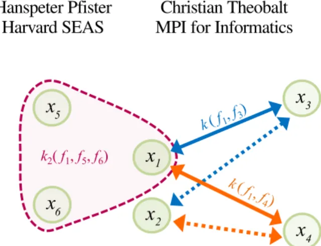
Figure 1. If two data pointsx1andx2are close on the domainM
off, then conventional regularizers enforce that the corresponding function valuesf1andf2in co-domainNoffare similar (fi≡f(xi)).
We assume that relationships between pairs of function evaluationsfi
andfjare represented by smooth functionsk(fi,fj), e.g., a similarity
measure. Our regularizer explicitly enforces thatk(f1,fj)andk(f2,fj)
are similar for anyj. For instance, ifk(f1,f3)is large asf1andf3are
similar, butk(f1,f4)is small asf1andf4are dissimilar (solid arrows),
then our algorithm enforces thatk(f2,f3)andk(f2,f4)are large and
small, respectively (dotted arrows), asx1andx2are close inM. The
same principle applies to high-order relationships: ifk2(f1, f5, f6)
represents a ternary relationship, e.g., a third-order correlation, the similarity ofk2(f1,f5,f6)andk2(f2,f5,f6)is enforced.
One example that benefits from this principle occurs when re-lationship labelsare provided. In semi-supervised orconstrained spectral clustering [12,14,18], the labels are provided not on the underlying cluster assignment functionfbut on the binary relationshipskbetween the function evaluations, asmust-linkor cannot-linklabels. These are exploited by applying conventional regularization onf with the condition that the constraints are satisfied. However, in this case, the relationship itself can also be a natural object to regularize (Fig.1). Applying homophily, if(x1,x3)must link, i.e., if they belong to the same cluster, then a
relationship functionkonNis defined such thatk(f(x1),f(x3))
is positive. For pointx2, which is close tox1inM, we expect
the relationship functionk(f(x2),f(x3))to be positive also.
In general, the relationship itself is not formally defined or observed; however, in many applications, certain relationships are manifested through a smooth function, where the number of arguments corresponds to the relationship degree, e.g., a distance metric is a function of two arguments.kcan be defined either directly from the data or from labels; either way, once the rela-tionship is defined, regularization is independent of the existence of labels and therefore applies generally to any learning problem.
1.1. Function-only and implicit relationships
We begin with a regularized empirical risk minimization framework wheref:M→Nminimizes the energy functional:
E(f)= X
i=1,...,s
l(yi,f(xi))+λR(f), (1) whereλis a regularization parameter,R:NM →R+ is the regularization functional that measures thecomplexity of the input function, andl:N×N→R+is the loss function. For simplicity, we assume thatN=Rnand adopt the squared loss: l(a,b) =ka−bk2, but our framework can be easily extended to
other convex loss functions. Extension to non-EuclideanN is also possible as discussed in Sec.2.2.
While a variety of semi-supervised learning algorithms can potentially benefit from our approach (see [4] for a comprehensive survey), we focus on the successful class of graph Laplacian-based approaches. One of the best-established classes of regularizers is based on applying differential operators tof:
RD(f)=
Z
M
k[Df](x)k2dV(x), (2)
where domainM is the Riemannian manifold as is common in semi-supervised learning, anddV(x)is the natural volume element ofM. IfDis the first-order differential operator dxd, thenRDis the familiarharmonic energyfunctional [2,16]:
Rh(f)=Z
M
k[∇f](x)k2
T∗
xdV(x), (3) with Riemannian connection ∇ in M, and cotangent space T∗
x:=Tx∗(M)ofM atx[11].
Roughly, this energy functional applies a differential operator to the input function and measures the corresponding squared norm. Minimizing this energy functional leads to asmooth function with smaller first-order magnitudes. WhenM is only indirectly observed through data point clouds,Rhis instantiated based on the graph Laplacian [2], the performance of which has been demonstrated in numerous applications.
Harmonic energy can be regarded as a first-order regularizer since it directly penalizes only variations off. For relationships, denoted by double brackets, e.g.,JA,BK, this roughly corresponds to minimizing the pair-wise deviations between self-relationships
Jf(x+dx)KandJf(x)K, whereJAKis simply as informative as A, with no consideration of relationships between entities.1
If we apply this first-order operator∇twice tof, i.e.,D=∇2,
we minimize the resulting second-order energy and penalize the deviations of the two pair-wise deviationsJf(x+dx),f(x)K
andJf(x−dx),f(x)K. This can be regarded as an example of a second-order relationship regularizer, with the relationship defined as the difference between two entities. Higher-order relationship regularizers then enforce smoothness on relationships involving more than two entities by increasing the order ofD. For
1A mathematically-precise relationship definition is obtained by equating
the relationship with a set functionF: 2M→
R. We do not adopt this definition since we focus on specific relationships instantiated through smooth kernels as defined in Sec.2.1. In this sense,JAKcan be identified with a set function defined on singletons, equivalent to a regular function onM.
instance, the state-of-the-artp-iterated Laplacian semi-norm[20] measures smoothness of(p−1)-th order relationships.
Rp(f)=Z
M
f(x)[∆pf](x)dV(x). (4) However, existing differential operator-based regularizers focus only onlocalrelationships. By construction,Df(x)is defined for an arbitrarily small open set containingx, and so it does not explicitly enforce smoothness over any pairJf(x),f(x
0)
K
andJf(x
00),f(x000)
Kof relationships when all four input points x,x0,x00,x000do not lie within a small neighborhood — even when xandx00are close. This property is shared by established regular-izers in Euclidean space (i.e.,Mis Euclidean): For instance, the well-known Gaussian kernel regularizer corresponds to Eq.2with Dbeing a combination of powers of the Laplacian operator [15].
Implicitly, any existing regularization functional regularizes any high-order relationships, as smoothness on f implies smoothness on pairsJf(x),f(x0)K. While apparently redundant, we will show experimentally that adding explicit control over relationship regularization increases utility over existing function-only regularizers.
The success of local high-order derivative-based regularizers supports this claim: In 1D space, minimizing the first-order derivative norm as a regularizer implicitly minimizes all high-order derivative norms, as the only null space of the first-order derivative operator is the space of constant functions (as these have zero high-order derivatives). Nevertheless, the use of high-high-order derivative-based regularizers, e.g., thin plate spline and Gaussian regularizers, is strongly supported by their empirical performances.
That high-order derivative-based regularizers can be con-sidered as local high-order relationship regularizers, coupled with the success of these approaches over first-order (or non-relationship) regularizers, leads us to investigate the potential of ‘longer-range’ relationship regularization. Among this various set of apparently-redundant regularizers, which leads to improved performance? We explore this potential and empirically validate thatexplicitlyexploiting rich structural information on non-local relationships improves existing regularization algorithms.
2. Relationship regularization
To begin, we focus on a specific class of relationships and discuss the ideal case where we knowM exactly. In Section
2.3, we present a practical algorithm for whenM is indirectly represented as a sampled point cloudX={x1,...,xu}.
2.1. Class of relationships
In many problems,Nhas relationship structure that is either canonically specified by the problem or is given implicitly. In clas-sification, the target space is the discrete space of class member-ships. In this case, the natural relationshipJf(x),f(x0)Kis binary: eithersame classordifferent class. In matching,Jf(x),f(x0)Kis eithermatchorno match.2In Markov random fields (MRF),N
can be explicitly provided with a pair-wise potentialp:N×N→ R, or ann-ary potentialq:Nn→R[10]. In many cases, these
relationships represent similarity between pairs orn-tuples of entities; in general, any non-metric relationship can be defined, e.g.,left oforon top offor generating topographic maps.
These relationships can be represented by ann-th order rela-tionship functionkdefined onNn, wherenis application specific. In principle, any relationship function can be regularized; for nu-merical optimization, we focus onkthat issmoothwrt. the input arguments (i.e.,k∈C∞(Nn)). Specifically, for semi-supervised learning, we use a Gaussian relationship functionk:
k(f(x),f(x0))=exp −(f(x)−f(x 0))2 σ2 f ! (5) whereσ2 f>0. We assume thatf∈C ∞(M), which we regularize as aided by relationships. We obtain the final class membership {−1,1}by thresholding the output space.
2.2. Regularization on relations
Our proposed regularizer assumes the general cases where Nis a Riemannian manifold (though many examples, including our demonstrations, are Euclidean inN). First, we discuss a straightforward approach which is not computationally practical for large problems. Then, we develop this intuition further to arrive at a computationally-affordable solution.
We construct the regularizer offbased on the regularization of relationshipkon the evaluations off. First, we construct the pullback function[11]f∗kofkbased onf:
f∗k(x,x0):=k(f(x),f(x0)). (6) This operation castsk, originally defined onN2, into a function
defined onM2so that it can be regularized based on the
differen-tial structure onM2: Sincef∗k∈C∞(M2), we can immediately
extend the harmonic energyRhand thep-iterated Laplacian semi-normRpas defined now onM2by noting thatf∗kcan be re-garded as a single-argument function on the product manifoldM2:
1) The tangent space for the point(x,x0)is defined based on the direct sum:T(x,x0):=Tx⊕Tx0; 2) The Riemannian metric is
de-fined bygM2(x1+x2,x01+x02) :=gM(x1+x2)+gM(x01+x02), which fixes the natural volume elementdV(x,x0); 3) Based on 1) and 2), the differential structure∇M2follows naturally from∇M. The resulting new energy is in the same form asRh(Eq.3) except that its domain is nowM2instead ofM:
Rprodk (f∗k)= Z M2 k[∇f∗k](x,x0)k2 T∗ (x,x0) dV(x,x0). (7) The biggest obstacle to apply this straightforward construction to semi-supervised learning is its high computational complexity. When approximatingRhandRpbased on a sampled point cloud of sizeu, the corresponding approximations are calculated based onu×umatrices (Sec.2.3). For the product manifoldM2, the approximations now require building regularization matrices of sizeu2×u2, which become infeasible even for moderateu.
Our approach is to make the roles ofxandx0asymmetric in the regularization. For a given pair-wise relationship function k, we construct an auxiliary single-argument functionhand the
corresponding pullback functionf∗has:
hy0(y):=k(y,y0)∈C∞(N), (8)
f∗hx0(x):=hf(x0)(f(x))∈C∞(M). (9)
Now, we define new extensions of harmonic energy functional andp-th iterated Laplacian energy functional as:
Rhk(f)= Z M Z M k∇f∗hx0(x)k2T∗ xdV(x)dV(x 0), (10) Rkp(f)= Z M Z M hx0(x)[∆pf∗hx0(x)]dV(x)dV(x0). (11)
For each fixedx0 in the function, f∗hx0(x)encodes the
relationship between f(x)andf(x0), and sincef∗hx0(x)is
a function of a single variable x ∈ M, ∇f∗hx0(x) lies in
Tx∗(M). This makes the interpretation of Eqs.10and11also straightforward: the inner integral measures the variation of f∗hx0(x)that corresponds to pair-wise relations between the
fixedx0and each value ofx. In particular, whenk(a,b)measures the Euclidean distance betweenaandb, the inner integral is zero only when the distances between each pairJf(x),f(x0)K
are identical for allx∈M. This does not require thatkis zero. Then, the outer integral averagesx0over the entireM.
For ann-th order relationship functionq, the corresponding Rq’s can be defined similarly through an n-times iterated integration: For each case, a pull-back function similar to f∗h
x0(x)is defined as aC∞ function onM. An important
advantage of this asymmetrization is that now the corresponding approximate regularization matrices retain the sizes ofu×u(see Sec.2.3) and accordingly they afford practical applications.
It should also be noted that currently, our regularizer does not exploit the potential differential structure of the target manifoldN. While the differential structure ofNis irrelevant in most applica-tions we foresee, for interested readers, we note that in principle, our regularizer can take this structure into account by pulling it back toM, i.e., to use thepullback connectionf∗∇N [16].
2.3. Approximating
Rkfrom a sampled point cloud
In many practical applications,Mis not directly observed but indirectly represented as a sampled point cloudX={x1,...,xu} and accordingly, we approximateRkbased on evaluations off onX. For a given relationship functionk, our approximate regularization functional toRh kis defined as: f Rh k(f)=tr[K >LK], (12) wheretr[·]is the trace,Kij:=k(f(xi),f(xj)), andL(u×u) is the graph Laplacian:
L=D−W, (13) where Wij = exp −kxi−xjk σ2 x
when xi, xj are k-nearest neighbors and 0 when not, σ2x is a hyper-parameter, andD is a diagonal matrix containing the column sums ofW. For exposition, we use the unnormalized graph Laplacian. However, our results straightforwardly extend to normalized graph Laplacian cases, which we use for all experiments (Sec.4.3).
discrete approximation off∗hxi(·), the convergence ofRf h
kto Rkcan be easily established based on the convergence results of the graph Laplacian to the Laplace-Beltrami operator [2,6]. Proposition 1.LetM be a connected, compact submanifold ofRM without boundary andXu={x1,...,xu} be sampled from a uniform distribution onM. Then, forf∈C∞(M)and k∈C∞(N×N)andσ2 x(u)=u − 1 m+2+α withα >0, lim u→∞ f Rh k(f) u3(σ2 x(u))m/2+1 =R h k(f) V(M)2, (14)
in probability, whereV(M)is the volume ofM.
Proof.The proof is similar to that of Theorem 4 by Zhou and Belkin [20]. Sincef∈C∞(M)andk∈C∞(N×N),f∗hx0∈
C∞(M). Then, applying the convergence result of graph Lapla-cian tof∗hxifor a fixedxi[2], we have∀xj∈X in probability,
lim u→∞ [LK[:,i]]j u(σ2 x(u))m/2+1 =∆f∗hxi(xj). (15) For Eq.14, we apply the law of large numbers and then Green’s identity [11] for a compact manifold without boundary to Eq.15:
Z M f∆gdV(x)=− Z M h∇f,∇giT∗ xdV(x). (16) For simplicity, we assume a uniform sample distribution on M. However, this result extends to non-uniform underlying probability distributionsPonMvia Hein et al. [6]. In this case, the integrand in Eq.10is weighted by the corresponding density.
Similarly toRh
k, the approximate regularization functional toRpkis defined as:
f
Rpk(f)=tr[K>LpK]. (17) Given Prop.2.3conditions, the convergence ofRfpktoRpkfollows
from Eq.16and the fact that∆f∈C∞(M)forf∈C∞(M).
3. Semi-supervised learning
Given the two regularizersRandRk (Eqs.3 and10or Eqs.4and11) and the loss function (l; Eq.1), we state our semi-supervised learning algorithm:
Ek(f)=(f−t)>H(f−t)+λ
1f>Gf+λ2tr[K>GK]
≈ X
i=1,...,s
l(yi,f(xi))+λ1Rh(f)+λ2Rhk(f), (18) wheref= [f(x1),...,f(xu)]>,His a diagonal matrix,Hii= 1 ifi-th data point is labeled (0otherwise),λ1andλ2are
regular-ization hyper-parameters, andGisLorLp. Fort, if thei-th data point is labeled,tiis the corresponding labelyi, or otherwise0. While the first two summands inEkare convex with respect tof, the third term is non-convex. We minimizeEkbased on con-jugate gradient (CG) descent. We set the initial solutionf0as the minimizer ofEkwithλ
2held fixed at 0, which can be analytically
computed. Hence, the entire optimization process is deterministic. With the Gaussian relationship function (Eq.5), the gradient
of each summand for thet-th function evaluation is: ∂(f−t)>H(f−t) ∂f = 2H(f−t) (19) ∂f>Gf ∂f = 2Gf (20) ∂tr[K>GK] ∂ft = 2tr[K>G∂K ∂ft ], (21) wheref=[f(x1),...,f(xu)]>and ∂Kij ∂ft = −2(fi−fj) σ2 f Kij ifi=t −2(fj−fi) σ2 f Kij else ifj=t. (22)
For (binary) classification problems,yi∈{−1,1}. In Sec.3.2, we discuss the dimensionality reduction problem where the output dimensionalitynis larger than1and accordinglyf(x)is a vector.
3.1. Sparsity
Our empirical explicit relationship regularizer enforces smoothness across every possible pairwise evaluation of the function f. This leads to a dense matrix Kin Eq.18. For large-scale problems, we can construct a sparse version of the regularizer by discarding the smoothness enforcement over the relationships that are evaluated for distant points, and focus only on local neighborhoods (not to be confused with the locality of the regularizer, i.e., neighborhood for graph Laplacian):
Ek S(f)=λ2 X i X jk (Kij−Kik)2Wjkgijgik, (23) wheregij=1ifxiandxjare in a specified neighborhoodNK andgij= 0, otherwise. When the neighborhood size is infinite (i.e.,g=1),Ek
Sis the same as the original regularizer in Eq.18. Otherwise,Ek
Senforces smoothness only for relationships that are defined for function evaluations of close input points.
3.2. Relationship labels and spectral embedding
For some applications, the relationshipsKthemselves are natural variables of interest, and so training labels can be user provided. For instance, in spectral embedding such as for cluster-ing and dimensionality reduction, e.g., in scientific visualization, wheref(x)∈Rnwithnbeing the desired dimensionality, the absolute value of the function f may be irrelevant while the relativespreadof the data are important. The user might provide expert rules to define which data points should be close to each other (must-link) or not (cannot-link). We can exploit this by penalizing the deviation ofKfrom the given relationship labelT:
Ek
Q(f)=k(K−T).Qk
2
F, (24) whereQij= 1if the labelTijis provided for a pair(i,j), and
Qij = 0otherwise. Tij = 1when f(xi)and f(xj)should be close to each other in the embedding space, andTij= 0 otherwise.A.Bis element-wise multiplication of two matrices AandB, andkAkFis the Frobenius norm ofA. In this case, our new energy functional is constructed as follows:
where we set the labeltand the initial search solutionf0of the optimization as the results of standard spectral embedding ob-tained from a graph Laplacian-based algorithm:f0=[e2,...,en] witheibeing thei-th eigenvector ofL. Since each outputf(x) is a vector, our relationship function is adapted accordingly:
k(f(x),f(x0))=exp −kf(x)−f(x 0)k2 σ2 f ! . (26) Minimizing Eq. 24 over f is different from independently minimizing it for each output dimension since the outputs are tied across the dimensions through the relationship labels (Eq.25), and the regularizer (Eq.12) is truly vector valued.
4. Experiments
We compare the performance of our explicit relationship regu-larization (ERR, Eqs.10and11) by adapting two existing implicit relationship regularizations (IRR, Eqs.3and4): classic graph Laplacian [2] and state-of-the-art iterated graph Laplacian [20]. To our knowledge, no algorithms exist which attempt to explicitly regularize relationships, even though they may implicitly attempt to do so (Sec.1.1). The purpose of our experiments is to show the improvement that can come from explicit relationship regulariza-tion, using standard and state-of-the-art approaches as evidence. As such, we conducted a semi-supervised learning experiment for pattern classification with a set of standard machine learning databases. Code will be made available on the web.
4.1. Semi-supervised classification
We use seven standard binary classification datasets for semi-supervised learning covering image digits (USPS), EEG signals (BCI), newsgroup categories (Text, Pcmac, Real-sim) and news reports (CCAT, GCAT) [4,20]. We randomly divide each dataset into three subsets: 50 labeled data points, 50 data points for vali-dation for hyper-parameter selection, and the remaining unlabeled data points are used for evaluation. We average error rates for 10 experiments with different sets of labeled examples. To demon-strate sparsity for large datasets (Sec.3.1), we use the 60,000 point large MNIST dataset, with binary labels obtained in the same way as for the USPS dataset [4]. Here,|NK|=200, while the number of labeled and validation data points were fixed at 300 each. Due to the large size of the problem, the iterated graph Laplacian was not applicable for neither IRR nor ERR since taking the power of a sparse (Laplacian) matrix tends to produce a denser matrix. Binary classification allows direct comparison of regulariza-tion performance and disregards multi-class combinaregulariza-tion method effects. However, to gain an insight into multi-class classification performance, we performed experiments with a 10-class dataset of 2,000 data points sampled from MNIST. For training and vali-dation, we used 50 labels for each class. To facilitate representing the multi-class outputs, we learn a vector-valued functionfand the corresponding relationship functionkas defined in Eq.26.
For IRR, there are three parameters: σ2
x,kN, thek-nearest neighborhood size for the graph Laplacian construction (Eq.13), and regularization parameterλ1. For ERR (Eq.10), there are
two more to be tuned:σ2
f for the Gaussian similarity relationship
functionk(Eq.5), and regularization parametersλ2. We first find
bounds forσ2x,kN, andλ1around the optimal for IRR; then, we
optimizeσf2andλ2for ERR. This resulted in the total number of
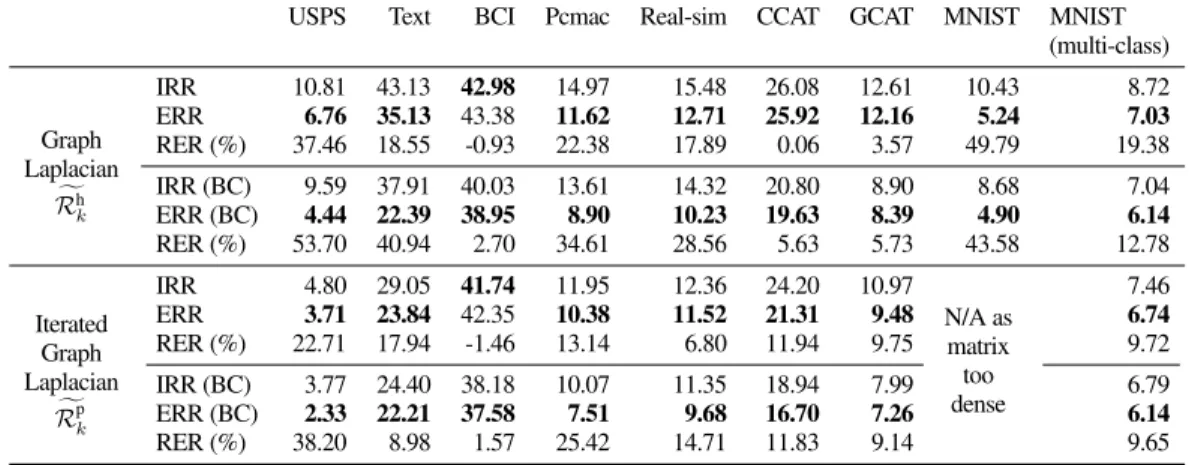
parameter evaluations for ERR being only slightly larger than that of IRR. ForRpk(Eq.11) there is an additional hyper-parameter pthat we fix at2throughout the entire set of experiments. Performance For all but one dataset, the error rate of ERR was lower than that of IRR when parameters were automatically chosen (Table1). This demonstrates the possible improvement of ERR over IRR and supports our claim that explicitly exploiting relationship information is useful. However, automatically optimizing the parameters with a limited number of labeled points can lead to overfitting (as observed in worse performance for ERR on BCI). Automatic tuning of hyper-parameters is still an open problem in semi-supervised learning where only a limited number of labeled examples are provided.
We also report the performance of both algorithms when best-case (BC) hyper-parameters are provided (odd row blocks), and the performance difference between ERR and IRR is more pronounced. This indicates that ERR can potentially lead to larger improvements over IRR when the parameters are tuned properly (e.g., through user interaction). If the error rate surface with respect to the hyper-parameters issmooth, then the user could decide the next search point based on the information gathered thus far. Our preliminary experiments showed that the error rate surface with respect to hyper-parameterissmooth. Accordingly, the active sampling strategy can indeed be exercised (Table1).
4.2. Spectral embedding
Our algorithm is a general regularizer for Riemannian man-ifolds, and also supports explicit relationship labels. We use dimensionality reduction and clustering applications to show this with MNIST, full USPS, and standard UCI clustering datasets (Diabetes, Iris, Wine, Breast Cancer Wisconsin (BCW), and Pendigits).Must-linkandcannot-linklabels are based on ground truths for selected pairs. Note that relationship labels areweakin that having a positive or negative labelTijfor a pairfiandfjdoes not reveal the corresponding class information for eitheryioryj.
In general, for unsupervised learning such as clustering and dimensionality reduction, automatic tuning of hyper-parameters is infeasible as there is no ground-truth information. Following experimental convention [3], we setkN=10andσ2xadaptively based on the average Euclidean distance of a point to itskN neighbors. In practice, the remaining hyper-parameters should be user tuned. To facilitate this process, we reduce the number of hyper-parameters to two, by first settingλ1=0(see Eq.25) and
tyingλ2andλ3by a new parameterλ02: We set the weightλ3
of relationship labels at a relatively large value10as these user labels should be regarded as quasi-hard constraints. The overall contribution of thesRrelation labels is controlled byλ02, replacing λ2byλ2/sR. Figure2shows that parameter tuning is feasible as performance varies smoothly with respect to the parameter space.
Again, while the hyper-parameters might be tuned based on user inspection in practice, to facilitate numerical evaluation for each dataset we randomly selectedsR=250labels and optimized
Table 1. Classification performance as error rate for implicit and explicit relationship regularization (IRR and ERR), versus both graph Laplacian (Rfh
k) and iterated graph Laplacian (Rf p
k) regularizers, with added best-case parameters (BC; Sec.4.1). Bold marks the best results. The performance
improvement of ERR over IRR is calculated as the reduction of error rate (RER) in %.
USPS Text BCI Pcmac Real-sim CCAT GCAT MNIST MNIST
(multi-class) Graph Laplacian f Rh k IRR 10.81 43.13 42.98 14.97 15.48 26.08 12.61 10.43 8.72 ERR 6.76 35.13 43.38 11.62 12.71 25.92 12.16 5.24 7.03 RER (%) 37.46 18.55 -0.93 22.38 17.89 0.06 3.57 49.79 19.38 IRR (BC) 9.59 37.91 40.03 13.61 14.32 20.80 8.90 8.68 7.04 ERR (BC) 4.44 22.39 38.95 8.90 10.23 19.63 8.39 4.90 6.14 RER (%) 53.70 40.94 2.70 34.61 28.56 5.63 5.73 43.58 12.78 Iterated Graph Laplacian f Rpk IRR 4.80 29.05 41.74 11.95 12.36 24.20 10.97 N/A as matrix too dense 7.46 ERR 3.71 23.84 42.35 10.38 11.52 21.31 9.48 6.74 RER (%) 22.71 17.94 -1.46 13.14 6.80 11.94 9.75 9.72 IRR (BC) 3.77 24.40 38.18 10.07 11.35 18.94 7.99 6.79 ERR (BC) 2.33 22.21 37.58 7.51 9.68 16.70 7.26 6.14 RER (%) 38.20 8.98 1.57 25.42 14.71 11.83 9.14 9.65
Figure 2. Clustering performance (error rate) of the proposed algorithm on USPS dataset with hyper-parametersσ2
fandλ2(λ02∗SR) that vary
in multiplicative intervals 2 and 3, respectively.
σf2andλ02based on their respective ground-truth error measures
(Sec.4.2.1). These parameter values are fixed acrossallsRvalues. For each value ofsR, we randomly sampled half the number of must-link and cannot-link labels, averaging error rates across 10 experiments. For comparison, we tuned the hyper-parameters of all competing algorithms (as described shortly) for each dataset and for each value ofsR, based on the ground-truth error rate, which is an advantage over our fixed parameters acrosssRvalues. 4.2.1 Clustering
From the optimizedf∗, the final cluster label is assigned to each data point by applyingk-means clustering onf∗. Sincek-means optimization is non-convex, we run it ten times with random ini-tialization and choose the result that minimizes thenormalized cut (NCut)[3] as it can be calculated without requiring any labels. We compare with the original spectral clustering, and three state-of-the-art algorithms which exploit explicit relationship labels: Con-strained Clustering via Spectral Regularization (CCSR) [12] and Flexible Constrained Spectral Clustering (CSP) [18] both optimize spectral energy (R) but under hard and soft constraints respec-tively (must-link and cannot-link), while Constrained 1-Spectral Clustering (COSC) [14] minimizes a continuous (L1) relaxation of the NCut under the same constraints. These algorithms
signifi-cantly outperform existing (relationship-) constrained approaches, as well as unconstrained clustering algorithms [12,14,18].
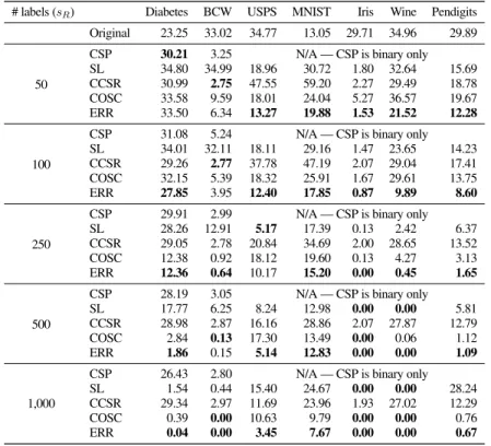
One major difference between those algorithms and ours is that they regularizefwith constraints, while our algorithm explicitly regularizes relationships. We also compare with the more classical Spectral Learning algorithm (SL) that encodes the constraints into the weight matrix in building the graph Laplacian [7]. For CCSR and CSP, we used the code provided by the authors on their web-sites. Since CSP is designed for binary clustering, we only report the corresponding results of binary datasets (Diabetes, BCW). The clustering error is defined by summing the occurrences of errors for each cluster: a data points is counted as an error if its label is different from the dominant label of the cluster to which it belongs. Performance All algorithms that exploit relationship labels significantly improved over original spectral clustering (Table2). The CSP and CCSR were especially good for BCW when the number of labelssRis small. However, they failed to show steady performance increases assRincreases. Further, for Diabetes, both algorithms showed much higher error rates than other algorithms. On average, SL showed better performance over CSP and CCSR. However, for some datasets, it showed significant error rate increases whensRis too large, which shows application limitation. Overall, COSC and our algorithm (ERR) demonstrated steady decreases of error rates assRincreases. However, except for one case (BCW forsR=500), our algorithm outperformed COSC by a large margin. For USPS, the error rates of COSC stayed high even whensR= 1,000: in the original spectral clustering result, multiple classes are merged into a single cluster, which leads to a single class dominating in multiple clusters. Classes 1 and 4 dominated in two clusters, respectively, and accordingly, classes 6 and 10 are absorbed. While ERR restored all classes whensR=500, COSC failed even whensR=1,000. 4.2.2 Dimensionality reduction
The target dimensionalitynwas set at 2 for all experiments, e.g., for visualization applications, though any dimensionality is possi-ble. We measured the error rate based on leave-one-out 1-nearest
Table 2. Clustering performance as error rate for different constrained clustering algorithms. # labels (sR) Diabetes BCW USPS MNIST Iris Wine Pendigits
Original 23.25 33.02 34.77 13.05 29.71 34.96 29.89
50
CSP 30.21 3.25 N/A — CSP is binary only
SL 34.80 34.99 18.96 30.72 1.80 32.64 15.69 CCSR 30.99 2.75 47.55 59.20 2.27 29.49 18.78 COSC 33.58 9.59 18.01 24.04 5.27 36.57 19.67 ERR 33.50 6.34 13.27 19.88 1.53 21.52 12.28
100
CSP 31.08 5.24 N/A — CSP is binary only SL 34.01 32.11 18.11 29.16 1.47 23.65 14.23 CCSR 29.26 2.77 37.78 47.19 2.07 29.04 17.41 COSC 32.15 5.39 18.32 25.91 1.67 29.61 13.75
ERR 27.85 3.95 12.40 17.85 0.87 9.89 8.60
250
CSP 29.91 2.99 N/A — CSP is binary only SL 28.26 12.91 5.17 17.39 0.13 2.42 6.37 CCSR 29.05 2.78 20.84 34.69 2.00 28.65 13.52 COSC 12.38 0.92 18.12 19.60 0.13 4.27 3.13
ERR 12.36 0.64 10.17 15.20 0.00 0.45 1.65
500
CSP 28.19 3.05 N/A — CSP is binary only SL 17.77 6.25 8.24 12.98 0.00 0.00 5.81 CCSR 28.98 2.87 16.16 28.86 2.07 27.87 12.79 COSC 2.84 0.13 17.30 13.49 0.00 0.06 1.12
ERR 1.86 0.15 5.14 12.83 0.00 0.00 1.09
1,000
CSP 26.43 2.80 N/A — CSP is binary only SL 1.54 0.44 15.40 24.67 0.00 0.00 28.24 CCSR 29.34 2.97 11.69 23.96 1.93 27.02 12.29 COSC 0.39 0.00 10.63 9.79 0.00 0.00 0.76 ERR 0.04 0.00 3.45 7.67 0.00 0.00 0.67
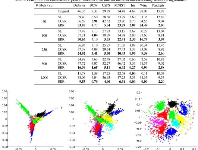
neighbor classification: For each point, we find its nearest neigh-bor and use the corresponding retrieved class label as the predicted label and measured the error rate. For comparison, we show the re-sults of CCSR and SL. While both CCSR and SL were originally developed for clustering, they first perform spectral embedding to a given target dimension and then apply conventional clustering therein. Their embedding parts can be used for dimensionality reduction by choosing the target dimension accordingly. Performance All algorithms improve over the original spectral dimensionality reduction (Table3), demonstrating the utility of relationship labels. CCSR was especially good for BCW, but it did not show noticeable improvement assRincreases. ERR and SL both showed steady error rate decreases while ERR significantly outperformed SL, demonstrating the utility of explicit relationship regularization. Figure3shows an example embedding.
4.3. Complexity
For all experiments, following conventions, the graph Laplacians are normalized. We set the number of conjugate gradient (CG) steps to 50. This provides a moderate trade-off between the performance and accuracy: While we observed a steady increase in accuracy as the number of CG steps increased for pattern classification experiments, the rate of increase dropped significantly past 50. As indicated by the form of the energy functional (Eq.12), when sparsity in relationships is not enforced (see Eq. 23), the time complexity of each gradient step is cubic in the number of data points. For pattern classification experiments with the USPS dataset (with 1500 data points), it took approximately 1.6 seconds for 50 CG step on NVIDIA GeForce
Table 4. Performance vs. sparsity (|NK|) for MNIST subsets
(s= 100,u= 2,000). GPU optimization negates the need for sparsity for these problem sizes.
|NK| 25 50 100 200 full ERR IRR
Error (%) 9.76 9.08 8.64 8.02 7.82 10.10
Time CPU (sec.) 3 10 21 38 35 1
Time GPU (sec.) - 3
-680 GPU, and 25 seconds on Intel Xeon 3.6GHz CPU; while the IRR took approximately 0.3 seconds on the same CPU: IRR can be solved analytically, while ERR must be solved iteratively.
4.4. Sparsity
To gain an insight into the sparsity/performance trade-off, we performed experiments on a small subset (u= 2,000) of the MNIST dataset such that direct performance comparison with dense regularization is possible (Table4). Performance degrades gracefully as|NK|decreases. For this small dataset, the processing time of the sparse system when|NK|=200is longer than the full ERR due to the sparsification overhead. However, the complexity grows roughly linearly with respect tou, and thus sparsity makes ERR applicable to large-scale datasets. In Table1, we show the results of the full MNIST dataset with|NK|=200.
5. Discussion
We have only evaluated the binary relationship functionkwith the single parameterσ2
f, and different potential relationship func-tion types could be explored. Further, we have only investigated
Table 3. Leave-one-out classification performance as error rate for different dimensionality reduction algorithms. # labels (sR) Diabetes BCW USPS MNIST Iris Wine Pendigits
Original 46.35 9.37 29.29 34.48 4.67 28.09 15.92 50 SL 39.40 6.50 28.68 33.29 3.60 31.35 12.88 CCSR 36.59 3.91 42.62 33.70 2.73 34.55 9.04 ERR 33.95 4.77 5.34 23.29 3.07 24.49 2.80 100 SL 37.49 7.13 27.93 33.15 3.67 30.28 13.04 CCSR 37.21 4.04 38.39 34.98 2.80 33.60 8.81 ERR 30.63 4.10 5.35 22.41 2.33 16.74 3.07 250 SL 36.93 7.10 25.85 31.05 1.87 20.34 11.45 CCSR 37.38 4.09 29.24 37.43 3.33 33.09 8.92 ERR 24.92 3.41 5.30 10.43 0.93 9.38 2.60 500 SL 24.88 3.63 22.48 27.02 0.60 2.58 10.82 CCSR 37.72 4.07 32.27 46.42 3.33 31.57 9.02 ERR 16.39 1.65 5.11 6.62 0.27 0.90 2.58 1,000 SL 11.78 1.39 17.25 22.68 0.00 0.11 10.03 CCSR 38.06 4.04 36.93 47.25 3.33 31.35 9.53 ERR 9.53 0.79 4.90 6.31 0.00 0.00 2.20 −0.05 0 0.05 −0.08 −0.06 −0.04 −0.02 0 0.02 0.04 0.06 0.08 −0.05 0 0.05 −0.08 −0.06 −0.04 −0.02 0 0.02 0.04 0.06 0.08 −0.2 −0.1 0 0.1 0.2 −0.25 −0.2 −0.15 −0.1 −0.05 0 0.05 0.1 0.15 0.2 1 2 3 4 5 6 7 8 9 10
Figure 3. Embedding results for full 10-class USPS dataset (sR= 100); plots show only 2,000 data points for better visibility.Left:Spectral embedding
(tin Eq.25).Middle:Minimizing 1) deviation fromt; 2) training error for relationship labels (Eq.24), and 3) conventional graph Laplacian regularization energy (Ek
MandR: Eqs.24and18withλ2=0).Right:Our proposal (EMk andRk: Eq.25). Error rates (left to right):28.30,27.53, and0.63.
binary relationship functions, andn-ary relationship functions are possible. In this case, theKmatrix in Eq.18is replaced by a tensor, and the problem complexity increases, though it may still be possible to handle these cases by enforcing sparsity (Sec.3.1).
For the specific case of binary relationship functions regu-larized by the graph Laplacian (which corresponds to pair-wise regularization), our regularization energy functional (Eq.23) can be regarded as a construction of a ternary relationship function: One can define a ternary clique as a summand of Eq.23:
q(fi,fj,fk)=(Kij−Kik)2Wjkgijgik. (27) In this way, our algorithm can be viewed as a special case of an MRF. While, in general, the optimization with a ternary relation-ship function is computationally very demanding, the asymmetric roles of three arguments in our clique (see the last paragraph of Sec.2.2) leads to a computationally affordable algorithm. In this respect, one of our main contributions is a method to construct a high-order clique from low-order cliques and the corresponding practical algorithm for semi-supervised learning.
In our semi-supervised learning experiments, we chose hyper-parameters based on separate validation sets. Heuristics can
help set some hyper-parameters, e.g., for spectral embedding, we setσ2
xbased on the average Euclidean distance of a point to its
kNneighbors (Sec.4.2). For USPS, the corresponding average clustering error rate was around 20% higher than when varying and manually selectingσ2
x. This suggests that the heuristic can trade accuracy with hyper-parameter optimization time.
6. Conclusion
We have investigated explicit relationship regularization, which, in addition to regularizing the function in semi-supervised learning, now regularizes the relationships between function eval-uations through smooth relationship functions. This approach im-proves performance by a large margin in semi-supervised classifi-cation and in constrained spectral clustering appliclassifi-cations, and facil-itates a related algorithm in semi-supervised dimensionality reduc-tion. We believe semi-supervised learning and constrained cluster-ing algorithms will increase in importance in vision, e.g., recent works in pose estimation [17], and video segmentation [8]. Future work should consider what role our explicit relationship regulariza-tion plays on the effect of the statistical model, e.g., error bound.
Acknowledgements
Kwang In Kim thanks EPSRC EP/M00533X/1 and EP/M006255/1, James Tompkin and Hanspeter Pfister thank NSF CGV-1110955, and James Tompkin and Christian Theobalt thank the Intel Visual Computing Institute.
References
[1] S. Agarwal, N. Snavely, I. Simon, S. M. Seitz, and R. Szeliski. Building Rome in a day. InProc. ICCV, 2009.1
[2] M. Belkin and P. Niyogi. Towards a theoretical foundation for Laplacian-based manifold methods. Journal of Com-puter and System Sciences, 74(8):1289–1308, 2005.2,4,5
[3] T. B¨uhler and M. Hein. Spectral clustering based on the graph p-Laplacian. InProc. ICML, pages 81–88, 2009.5,6
[4] O. Chapelle, B. Sch¨olkopf, and A. Zien. Semi-Supervised Learning. MIT Press, Cambridge, MA, 2006.2,5
[5] S. Ebert, D. Larlus, and B. Schiele. Extracting structures in image collections for object recognition. InProc. ECCV, pages 720–733, 2010.1
[6] M. Hein, J.-Y. Audibert, and U. von Luxburg. From graphs to manifolds - weak and strong pointwise consistency of graph Laplacians. InProc. COLT, pages 470–485, 2005.4
[7] S. D. Kamvar, D. Klein, and C. D. Manning. Spectral learning. InProc. IJCAI, pages 561–566, 2003.6
[8] A. Khoreva, F. Galasso, M. Hein, and B. Schiele. Learning must-link constraints for video segmentation based on spectral clustering. InProc. GCPR, pages 701–712, 2014.8
[9] K. I. Kim, J. Tompkin, M. Theobald, J. Kautz, and C. Theobalt. Match graph construction for large image databases. InProc. ECCV, pages 272–285, 2012.1
[10] J. Lafferty, A. McCallum, and F. Pereira. Conditional ran-dom fields: probabilistic models for segmenting and labeling sequence data. InProc. ICML, pages 282–289, 2001.2
[11] J. M. Lee. Riemannian Manifolds- An Introduction to Curvature. Springer, New York, 1997.2,3,4
[12] Z. Li, J. Liu, and X. Tang. Constrained clustering via spectral regularization. InProc. CVPR, pages 421–428, 2009.1,6
[13] M. McPherson, L. Smith-Lovin, , and J. M. Cook. Birds of a feather: Homophily in social networks. Annual Review of Sociology, 27:415–444, 2001.1
[14] S. Rangapuram and M. Hein. Constrained 1-spectral clustering. JMLR W&CP (Proc. AISTATS), 22:1143–1151, 2012.1,6
[15] B. Sch¨olkopf and A. Smola. Learning with Kernels. MIT Press, Cambridge, MA, 2002.2
[16] F. Steinke, M. Hein, and B. Sch¨olkopf. Nonparametric regression between general Riemannian manifolds. SIAM Journal on Imaging Sciences, 3(3):527–563, 2010.2,3
[17] D. Tang, T.-H. Yu, and T.-K. Kim. Real-time articulated hand pose estimation using semi-supervised transductive regression rorests. InProc. ICCV, pages 3224–3231, 2013.
1,8
[18] X. Wang and I. Davidson. Flexible constrained spectral clustering. InProc. SIGKDD, pages 563–572, 2010.1,6
[19] D. Zhou, O. Bousquet, T. N. Lal, J. Weston, and B. Sch¨olkopf. Learning with local and global consistency. InNIPS, pages 1330–328, 04.1
[20] X. Zhou and M. Belkin. Semi-supervised learning by higher order regularization. JMLR W&CP (Proc. AISTATS), pages 892–900, 2011.2,4,5
[21] X. Zhu, Z. Ghahramani, and J. Lafferty. Semi-supervised learning using Gaussian fields and harmonic functions. In Proc. ICML, pages 912–919, 2003.1