HAL Id: hal-02311256
https://hal.archives-ouvertes.fr/hal-02311256
Submitted on 10 Oct 2019
HAL
is a multi-disciplinary open access
archive for the deposit and dissemination of
sci-entific research documents, whether they are
pub-lished or not. The documents may come from
teaching and research institutions in France or
abroad, or from public or private research centers.
L’archive ouverte pluridisciplinaire
HAL, est
destinée au dépôt et à la diffusion de documents
scientifiques de niveau recherche, publiés ou non,
émanant des établissements d’enseignement et de
recherche français ou étrangers, des laboratoires
publics ou privés.
A New Preconditioner that Exploits Low-Rank
Approximations to Factorization Error
Nicholas J. Higham, Théo Mary
To cite this version:
Nicholas J. Higham, Théo Mary. A New Preconditioner that Exploits Low-Rank Approximations
to Factorization Error. SIAM Journal on Scientific Computing, Society for Industrial and Applied
Mathematics, 2019, 41 (1), pp.A59-A82. �10.1137/18M1182802�. �hal-02311256�
NICHOLAS J. HIGHAM AND THEO MARY
Abstract. We consider ill-conditioned linear systemsAx= b that are to be solved iteratively, and assume that a low accuracy LU factorizationA≈LbUbis available for use in a preconditioner. We
have observed that for ill-conditioned matricesAarising in practice,A−1 tends to be numerically low rank, that is, it has a small number of large singular values. Importantly, the error matrix
E=Ub−1Lb−1A−Itends to have the same property. To understand this phenomenon we give bounds
for the distance fromE to a low-rank matrix in terms of the corresponding distance forA−1. We then design a novel preconditioner that exploits the low-rank property of the error to accelerate the convergence of iterative methods. We apply this new preconditioner in three different contexts fitting our general framework: low floating-point precision (e.g., half precision) LU factorization, incomplete LU factorization, and block low-rank LU factorization. In numerical experiments with GMRES-based iterative refinement we show that our preconditioner can achieve a significant reduction in the number of iterations required to solve a variety of real-life problems.
Key words. matrix factorization, preconditioning, low-rank approximations, mixed precision iterative refinement, GMRES
AMS subject classifications. 65F05, 65F08, 65F10, 68W20
1. Introduction. We consider the iterative solution of a linear systemAx=b, whereA∈Rn×nis nonsingular. A widely used approach is to compute a low accuracy
LU factorizationA=LbUb+∆Aand use the approximate inverse factors Ub−1Lb−1 as
a preconditioner. However, the rate of convergence of the iterative method strongly depends on the matrix properties, such as the distribution of its singular values. IfA is ill conditioned the preconditioned iteration may converge slowly or not at all. In such a situation, we may have no other choice than to compute a more accurate LU factorization, which is likely to be too expensive for large-scale problems.
The objective of this article is to present a novel and yet general preconditioner that builds on a given approximate LU factorization and can be effective even for ill-conditioned systems. This preconditioner is based on the following key observation: ill-conditioned matrices that arise in practice often have a small number of small
singular values. The inverse of such a matrix has a small number of large singular
values and so is numerically low rank. This observation suggests that the error matrix E=Ub−1Lb−1A−I=Ub−1Lb−1∆A≈A−1∆A
is of interest, because we may expectE to retain the numerically low-rank property of A−1. The main contributions of this article are to investigate theoretically and experimentally whether E is indeed numerically low rank and to describe how to exploit this property to accelerate the convergence of iterative methods by building a preconditioner based on a low-rank approximation toE.
We begin, in section2, by describing the general framework for our analysis and providing three examples of algorithms that fit within the framework: low floating-point precision (for example, half precision) LU factorization, incomplete LU fac-torization, and block low-rank LU factorization. We also describe the experimental
∗Version of August 22, 2018. Funding: This work was supported by Engineering and Physical Sciences Research Council grant EP/P020720/1, The MathWorks, and the Royal Society. The opinions and views expressed in this publication are those of the authors, and not necessarily those of the funding bodies.
setting of the following sections. In section3 we derive sufficient conditions for the error matrix to be numerically low rank. In section4we propose a new preconditioner based on a low-rank approximation to the error. In section5we analyze experimen-tally how this preconditioner can accelerate the solution of linear systems in the three contexts mentioned above. We use GMRES-based iterative refinement (GMRES-IR) as our iterative method. Concluding remarks are given in section6.
Throughout this article, the unsubscripted normk · kdenotes the 2-norm. 2. General framework and three applications. We first describe the general framework to which the theory and algorithms developed in this article apply. We then provide three examples of widely used algorithms that fit within the framework: low floating-point precision LU factorization, incomplete LU factorization, and block low-rank LU factorization. We finally describe the experimental setting used in the following sections.
2.1. General framework description. We consider a linear systemAx=b, whereA∈Rn×n is nonsingular. We assume an approximate LU factorization
(2.1) A=LbUb+∆A
can be computed, but we do not make any assumption on how it is computed, nor do we assume∆Ato have any special structure. We define the error matrix as
E=Ub−1Lb−1A−I=Ub−1Lb−1∆A.
We will show theoretically and experimentally thatE is likely to have low numerical rank1 when A is ill conditioned (that is, κ(A) = kAkkA−1k 1). Note that A being ill conditioned is not a strict requirement of our framework, but the algorithms we design can cope with such matrices; therefore, in this article, we mostly consider ill-conditionedA.
2.2. Low floating-point precision LU factorization. The use of half or sgle precision floating-point arithmetic in mixed-precision algorithms is becoming creasingly common. In particular, half-precision arithmetic is attracting growing in-terest now that it has started to become available in hardware [13], [14].
A natural way to exploit a low precision LU factorization is with iterative re-finement. Carson and Higham [6] investigate iterative refinement in three precisions. They show that if the working precision u is double precision, the LU factors are computed in half precision, and residuals are computed in quadruple precision then convergence of the refinement process is guaranteed if κ(A)≤104 and backward er-rors and forward erer-rors of orderu will be produced. They also show that, by using GMRES preconditioned with the LU factors to solve for the correction term, the limit on κ(A) can be relaxed to 1012 or 1016 in order to ensure a forward error or back-ward error of order u, respectively. Algorithm 2.1 summarizes this GMRES-based iterative refinement (GMRES-IR), which was originally proposed in a form using two precisions [5].
While GMRES-IR requires only a small number of iterative refinement steps (outer iterations) whenκ(A) satisfies the required bounds, the number of iterations in the GMRES solves (inner iterations) can be large. In this article, we will demonstrate how the new preconditioner proposed in section4 can help to reduce the number of inner iterations and therefore widen the range of tractable problems.
Algorithm 2.1 GMRES-based iterative refinement with precisionsuf, u, andur.
1 Compute LU factorization of Aat precisionuf.
2 SolveAx1=bat precisionuf using the LU factors and storex1 at precisionu.
3 while not convergeddo
4 Computeri=b−Axi at precisionur and roundri to precisionu.
5 SolveAde i≡Ub−1Lb−1Adi=Ub−1Lb−1riat precisionuusing GMRES, with matrix–vector products withAecomputed at precisionur.
6 xi+1=xi+di at precisionu.
7 end while
2.3. Incomplete LU factorization. The LU factors of a sparse matrix can be much less sparse than the matrix, because of fill-in, potentially making the factoriza-tion too expensive. This problem can be alleviated by using fill-reducing reorderings of the matrix, such as minimum degree, minimum fill, and nested dissection. However, the amount of fill-in can still be quite large in many practical applications.
A widely used alternative approach is to compute an incomplete LU (ILU) fac-torization [27, sec. 10.3], in which the sparsity of the LU factors is kept under a given threshold. For example, ILU(0) forces LbUb to have the same sparsity pattern as A.
More generally, the sparsity of the computed factors can be controlled by a tolerance τ, where filled entries of magnitude less thanτ(relative to the norm ofA) are dropped. For large values of τ, ILU-based preconditioners may yield slow convergence of the iterative method. We will show how our new preconditioner, used in conjunction with an ILU preconditioner, can overcome this obstacle.
2.4. Block low-rank LU factorization. In numerous scientific applications, such as the solution of partial differential equations, the matrices resulting from the discretization of the physical problem have been shown to possess a low-rank prop-erty [4]: suitably defined off-diagonal blocks of their Schur complements can be ap-proximated by low-rank matrices. This property can be exploited to provide a sub-stantial reduction of the complexity of matrix factorizations.
Several matrix representations—so-called low-rank formats—have been proposed in the literature. Most of them fit within our general framework, but we will focus on the block low-rank (BLR) format [1], [2], [3]. The BLR format is based on a flat 2D blocking of the matrix that is defined by conveniently clustering the associated unknowns. A BLR representationAeof a dense matrixA has the form
(2.2) Ae= A11 Ae12 · · · Ae1p e A21 · · · ... .. . · · · . .. ... e Ap1 · · · App ,
where each off-diagonal blockAij of sizemi×nj and numerical rankkτij is approxi-mated by a low-rank productAeij=XijYijT, whereXij ismi×kτij andYij isnj×kτij. The Aeij approximation of each block can be computed in different ways. We have chosen to use a truncated QR factorization with column pivoting, which is a QR factorization with column pivoting that is truncated as soon as a diagonal coefficient of theRfactor falls below a prescribed thresholdτ, referred to as the BLR threshold. The BLR thresholdτ controls the accuracy of the factorization.
In order to perform the LU factorization of a dense BLR matrix, the standard LU factorization has to be modified so that the low-rank blocks can be exploited to reduce the number of operations. Many such algorithms can be defined, depending on where the compression step (the introduction of the low-rank approximations) is performed. In this article, we will consider the CUFS variant, introduced in [2]. As described in [2], the CUFS variant achieves the lowest complexity of all BLR variants by performing the compression as early as possible.
Using the BLR factorization as an approximate LU factorization has been shown to make an efficient preconditioner for iterative methods such as GMRES, outperform-ing both traditional iterative and direct methods for many applications of practical interest [22]. We will show that our low-rank approximation to the factorization error can improve the performance of the BLR preconditioner.
2.5. Experimental setting. The numerical results have been obtained in MAT-LAB R2017b on a laptop computer equipped with 8 GB of memory and a four-core Intel i5-6300U running at 2.40GHz.
Our experiments use four different precisions of IEEE standard arithmetic: half-precision, with unit roundoffu= 4.9×10⁻⁴, for which we used the MATLAB fp16 class from the Cleve Laboratory toolbox [25]; single precision (u= 6.0×10⁻⁸) and double precision (u = 1.1×10⁻¹⁶); and quadruple precision (u = 9.6×10⁻³⁵), for which we use the Advanpix Multiprecision Computing Toolbox [26].
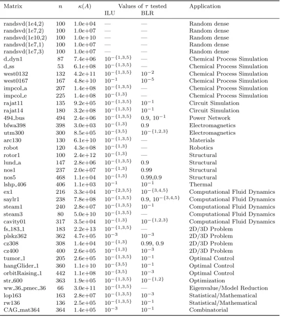
We will consider a large set of both random dense and real-life sparse matrices coming from a variety of applications. The randsvd matrices were generated with the MATLABgalleryfunction, usingrng(1)to seed the random number generator. All the other matrices come from the SuiteSparse Matrix Collection (previously called the University of Florida Sparse Matrix Collection) [9]. The full list is provided in Table2.1.
The matrices are of relatively small size. We are mainly interested in the theoreti-cal and numeritheoreti-cal behavior of the algorithms; their high performance implementation is not our focus here. We will, however, explain why the proposed algorithms are expected to perform well on large-scale problems and in parallel computing environ-ments.
Throughout the rest of this article, we will specify between parentheses after each matrix name which type of approximate LU factorization was performed: half precision LU factorization (fp16), incomplete LU factorization (ILU), or block low-rank LU factorization (BLR). For ILU, we used the MATLAB ilu function with threshold partial pivoting, withsetup.type = ‘ilutp’and drop toleranceτ.
Table2.1indicates which type of factorization was tested on which matrices. The fp16 factorization was tested on the full set; the ILU and BLR factorizations were tested on a subset of matrices with values of τ varying between 10−1 and 10−5 for ILU and between 0.99 and 10−5 for BLR. This leads to a total of 163 tests on 40 matrices.
3. Bounds for the numerical rank of the error matrix. In this section, we investigate theoretically and experimentally the numerical rank of the error matrix E =M−1A−I, whereM−1 is some preconditioner that approximatesA−1. In our LU-based preconditioner context,M =LbUb, but the analysis presented in this section
does not use the fact that the preconditioner M is based on an approximate LU factorization, so we writeM to keep the analysis general.
Table 2.1: The test matrices, indicating for each one which of ILU and BLR was tested and the corresponding values of the drop tolerance or the BLR thresholdτ.
Matrix n κ(A) Values ofτ tested Application
ILU BLR
randsvd(1e4,2) 100 1.0e+04 — — Random dense randsvd(1e7,2) 100 1.0e+07 — — Random dense randsvd(1e10,2) 100 1.0e+10 — — Random dense randsvd(1e7,1) 100 1.0e+07 — — Random dense randsvd(1e7,3) 100 1.0e+07 — — Random dense
d dyn1 87 7.4e+06 10−{1,3,5} — Chemical Process Simulation d ss 53 6.1e+08 10−{1,3,5} — Chemical Process Simulation west0132 132 4.2e+11 10−{1,3,5} 10−2 Chemical Process Simulation west0167 167 4.8e+10 10−1 10−5 Chemical Process Simulation impcol a 207 1.4e+08 10−{1,3,5} — Chemical Process Simulation impcol e 225 1.4e+08 10−{1,3} — Chemical Process Simulation rajat11 135 9.2e+05 10−{1,3,5} 10−1 Circuit Simulation
rajat14 180 3.2e+08 10−{1,3,5} 10−1 Circuit Simulation 494 bus 494 2.4e+06 10−{1,3,5} 0.9, 10−1 Power Network bfwa398 398 3.0e+03 10−{1,3} 0.9 Electromagnetics utm300 300 8.5e+05 10−{3,5} 10−{1,2,3} Electromagnetics arc130 130 6.1e+10 10−{1,3,5} — Materials robot 120 4.3e+08 10−{1,3} — Robotics rotor1 100 2.4e+12 10−{1,3} — Structural lund a 147 2.8e+06 10−{1,3,5} 0.9 Structural nos1 237 2.0e+07 10−{1,3} 0.99 Structural nos5 468 1.1e+04 10−{1,3} 0.99,0.9 Structural lshp 406 406 1.1e+03 10−1 10−1 Thermal
ex1 216 3.3e+04 10−{2,3,5} 10−{3,4,5} Computational Fluid Dynamics saylr1 238 7.8e+08 10−{1,3,5} 0.9, 10−{3,4,5} Computational Fluid Dynamics steam1 240 2.8e+07 10−{1,3,5} 10−1 Computational Fluid Dynamics steam3 80 5.0e+10 10−{1,3,5} — Computational Fluid Dynamics cavity01 317 3.5e+04 10−{1,3} 10−{1,2,3} Computational Fluid Dynamics fs 183 1 183 2.2e+13 10−{1,3,5} — 2D/3D Problem
plskz362 362 4.7e+05 10−3 10−3 2D/3D Problem cz308 308 1.4e+04 10−{1,3} 0.99, 0.9 2D/3D Problem cz400 400 2.6e+05 10−{1,3} 10−3 2D/3D Problem tumor 1 205 2.6e+05 10−{1,3,5} 10−1 Optimal Control hangGlider 1 360 1.1e+10 10−{3,5} 10−1 Optimal Control orbitRaising 1 442 1.1e+08 10−{3,5} 10−3 Optimal Control str 600 363 1.9e+05 10−{1,3,5} 10−{1,2} Optimization
ww 36 pmec 36 66 3.0e+11 10−{1,3,5} — Eigenvalue/Model Reduction lop163 163 2.8e+07 10−{1,3,5} 10−3 Statistical/Mathematical rw136 136 2.5e+05 10−{1,3,5} 10−1 Statistical/Mathematical CAG mat364 364 1.4e+05 10−3 10−1 Combinatorial
Definition 3.1. Let A∈Rn×n be nonzero. Fork≤n, the rank-kaccuracy ofA
is (3.1) εk(A) = min Wk kA−Wkk kAk : rankWk≤k .
We call Wk of rank k an optimal rank-k approximation to A if Wk achieves the
minimum in (3.1). The numerical rank ofA at accuracyε, denoted bykε(A), is
The matrix Ais of low numerical rank ifεk(A)1 for somekn.
LetXΣYT denote the singular value decomposition (SVD) ofA, and let σ i(A) be the ith largest singular value. By the Eckart–Young–Mirsky theorem [11], [20, p. 468], [24], kA−Wkkis minimized2forWk =X:,1:kΣ1:k,1:kY:,1:kT , which yields
(3.2) εk(A) =
σk+1(A)
σ1(A)
.
As stated in the introduction, we have observed that ill-conditioned matrices often have a numerically low-rank inverse. We now assume that A−1 is numerically low rank and seek conditions under which the error E = M−1∆Aretains this low-rank property. To that end, we have to answer two questions: isM−1numerically low rank ifA−1is numerically low rank? And isE numerically low rank ifM−1is numerically low rank?
To answer the first question, we considerM as an additive perturbation ofA. We need the following lemma.
Lemma 3.2. Let X ∈Rn×n andX+∆X∈Rn×n be nonsingular. Then
(3.3) σi(X+∆X)≤σi(X) 1 +kX−1∆Xk, 1≤i≤n.
Proof. Apply inequality (3.3.26) from [19] to X andX(I+X−1∆X).
We apply the lemma twice. First, recallingA=M+∆Aand takingX =M and ∆X=∆Ain (3.3) yields (for alli≤n)
(3.4) σi(A)≤σi(M) 1 +kM−1∆Ak
. Second, takingX =A and∆X=−∆Ain (3.3) yields (3.5) σi(M)≤σi(A) 1 +kA−1∆Ak.
We can now answer the first question with the following theorem.
Theorem 3.3. Let A=M +∆A∈Rn×n be nonsingular. The rank-k accuracy
of M−1 satisfies
(3.6) εk(M−1)≤βgβsεk(A−1), 1≤k≤n,
withβg= 1 +kA−1∆Ak andβs= 1 +kM−1∆Ak.
Proof. For allk≤n−1, by (3.2) we have εk(M−1) εk(A−1) =σk+1(M −1)σ 1(A−1) σ1(M−1)σk+1(A−1) = σn(M)σn−k(A) σn−k(M)σn(A) . Bounding the numerator with (3.4) and (3.5) yields the result.
Theorem3.3states that ifkA−1∆AkandkM−1∆Akare not too large thenM−1 will retain the low-rank property ofA−1. The quantityβ
g = 1 +kA−1∆Ak bounds how much the “perturbed” singular values ofM can grow with respect to those ofA by (3.5). Conversely,βs= 1 +kM−1∆Akbounds how much they can shrink by (3.4). The inequality (3.6) is sharp in a scenario where σn(A) = σ1(A−1)−1 grows by a
2This result is usually stated for the Frobenius norm, but actually holds for any unitarily invariant norm.
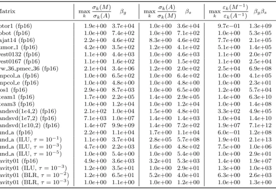
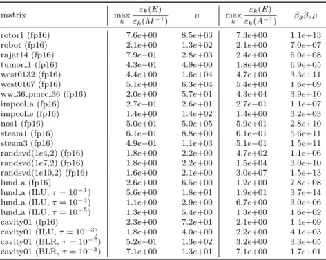
Table 3.1: Ratios and corresponding bounding quantities for a selection of matrices, where the LU factorization is computed in half precision or as an incomplete LU factorization or BLR factorization. Matrix max k σk(M) σk(A) βg max k σk(A) σk(M) βs max k εk(M−1) εk(A−1) βgβs rotor1 (fp16) 1.9e+00 3.7e+04 1.0e+00 3.6e+04 9.7e−01 1.3e+09 robot (fp16) 1.0e+00 7.4e+02 1.0e+00 7.1e+02 1.0e+00 5.3e+05 rajat14 (fp16) 2.2e+00 4.6e+02 8.3e+00 4.6e+02 7.7e+00 2.1e+05 tumor 1 (fp16) 4.2e+00 3.5e+02 1.2e+00 4.1e+02 5.1e+00 1.4e+05 west0132 (fp16) 1.1e+00 4.4e+03 1.0e+00 4.6e+03 1.1e+00 2.0e+07 west0167 (fp16) 1.1e+00 1.6e+02 1.0e+00 1.5e+02 1.1e+00 2.5e+04 ww 36 pmec 36 (fp16) 2.1e+04 3.4e+06 1.2e+00 2.0e+02 2.5e+04 6.9e+08 impcol a (fp16) 1.0e+00 6.5e+02 1.0e+00 6.4e+02 1.0e+00 4.1e+05 impcol e (fp16) 1.0e+00 4.8e+00 1.0e+00 4.8e+00 1.0e+00 2.3e+01 nos1 (fp16) 2.9e+00 8.7e+03 1.0e+00 6.5e+00 1.2e+00 5.7e+04 steam1 (fp16) 1.7e+00 2.2e+05 1.4e+00 2.9e+05 1.4e+00 6.3e+10 steam3 (fp16) 1.0e+00 1.2e+04 1.0e+00 1.2e+04 1.0e+00 1.4e+08 randsvd(1e4,2) (fp16) 2.1e+02 1.0e+04 1.5e+00 4.8e+01 3.3e+02 4.9e+05 randsvd(1e7,2) (fp16) 7.1e+03 1.0e+07 1.4e+00 1.4e+03 1.0e+04 1.4e+10 randsvd(1e10,2) (fp16) 1.4e+07 9.9e+09 1.4e+00 7.2e+02 1.9e+07 7.1e+12 lund a (fp16) 2.2e+00 1.1e+04 1.7e+00 1.1e+04 6.0e−01 1.2e+08 lund a (ILU,τ= 10−1) 1.1e+00 3.7e+04 2.8e+05 5.7e+08 1.9e+01 2.1e+13 lund a (ILU,τ= 10−3) 4.7e+00 2.2e+03 1.6e+00 4.8e+02 7.5e+00 1.0e+06 lund a (ILU,τ= 10−5) 1.0e+00 5.4e+00 1.0e+00 5.4e+00 1.0e+00 2.9e+01 cavity01 (fp16) 4.9e+00 3.6e+03 3.2e+01 5.3e+03 1.4e+00 1.9e+07 cavity01 (ILU,τ= 10−3) 1.2e+00 3.5e+01 1.0e+00 2.9e+01 1.3e+00 1.0e+03 cavity01 (BLR,τ= 10−2) 1.2e+00 6.5e+01 5.2e+00 4.0e+01 6.3e+00 2.6e+03 cavity01 (BLR,τ= 10−3) 1.0e+00 1.1e+00 1.0e+00 1.2e+00 1.0e+00 1.3e+00
factorβg andσn−k(A) =σk+1(A−1)−1shrinks by a factorβs. It is not clear whether this scenario is attainable. In any case the bound (3.6) is very pessimistic in practice. Numerical experiments are reported in Table 3.1 for a subset of the matrices, with the LU factors computed either in half precision or in double precision as an incomplete LU factorization or BLR factorization. For all these matrices, A−1 has low numerical rank. We see that the singular values of M are usually of the same order of magnitude as those of A, so thatM−1 remains of low numerical rank. The bound (3.6) is usually weak by three orders of magnitude or more, but depending on the matrix, it can still imply a low numerical rank. A possible explanation for the bound (3.6) being weak is that βgβs is the same for all k, whereas the value
εk(M−1)/εk(A−1) itself depends onk. It may thus not matter if εk(M−1)/εk(A−1) is large for a large value ofk, since we are only interested in smallk.
We now turn to our second question: assuming M−1 is numerically low rank, when can we expectE =M−1∆Aalso to be numerically low rank? We answer this question with the following theorem.
Theorem 3.4. LetA=M+∆A∈Rn×nbe nonsingular. The errorE=M−1∆A
satisfies (3.7) εk(E)≤µεk(M−1), 1≤k≤n, with (3.8) µ= kM −1k k∆Ak kM−1∆Ak .
Proof. Let Wk be an optimal rank-k approximation of M−1, so that kM−1−
Wkk=εk(M−1)kM−1k. ThenEk=Wk∆Ahas rank at mostk and therefore
εk(E)≤ kE−Ekk kEk = k(M−1−W k)∆Ak kEk ≤εk(M −1)kM− 1k k∆Ak kEk , as required.
Explaining the role ofµis less straightforward than forβgandβs. To clarify the role of µ, we compute an upper bound ¯µ= minkµ¯k whose mathematical meaning is easier to grasp. The following theorem states that unless∆Ais very special,µshould be of moderate size.
Theorem 3.5. The quantityµF =kM−1kk∆Ak/kEkF, which differs fromµonly
in that the Frobenius norm ofE is taken rather than the2-norm, is bounded by
(3.9) µF ≤µ¯k= σn+1−k(M) σn(M) k∆Ak kPk∆Ak , 1≤k≤n,
where Pk =XkXkT, Xk = [xn+1−k, . . . , xn], and xj is the left singular vector
corre-sponding to the jth largest singular value ofM.
Proof. The proof draws its inspiration from [7]. Let XΣYT be an SVD of M,
with σ1 ≥ · · · ≥ σn. Then, with xj and yj denoting the jth columns of X and Y, respectively, E=Y Σ−1XT∆A= n X i=1 1 σi yi xTi∆A . Thus, for allk≤n,
kEk2 F ≥ n X i=n+1−k 1 σ2 i kyik2kxTi ∆Ak2≥ 1 σ2 n+1−k n X i=n+1−k kxT i∆Ak2= 1 σ2 n+1−k kPk∆Ak2. We can therefore boundµF for allk≤nby
µF = k∆Ak σnkEkF ≤σn+1−k σn k∆Ak kPk∆Ak , as required.
Theorem 3.5 tells us that µF will be small when ∆A is a “typical” matrix: one having a significant component in the subspace span(Xk) for somek such that
σn+1−k(M)≈σn(M). Note that the proof requires us to take the Frobenius norm ofE, which is in general greater than its 2-norm (and thusµF ≤µ). However, since
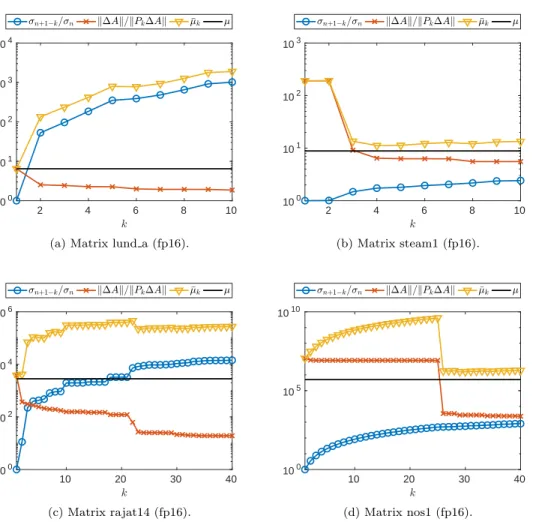
E is expected to be numerically low rank, kEk ≈ kEkF should hold. Thus, we can also expect µ ≈ µF to be small. Figure 3.1 plots the values of k∆Ak/kPk∆Ak,
σn+1−k(N)/σn(M), and ¯µk as a function of k for four example matrices, where
M =LbUb is from an fp16 LU factorization. In the first two cases (matrices lund a and
steam1),∆A=A−LbUb is a typical matrix and thusµ is small. However, for some
matrices (e.g., rajat14 and nos1 in Figure3.1),∆Aturns out to be special and leads to a largeµ. Nevertheless, for all the matrices studied, the bound (3.7) is never sharp whenµis large (see the second column of Table3.2).
We now build a matrix for which the µbound (3.7) is both large and sharp, to prove that it cannot be improved without further assumptions on the matrix. Gener-ating a matrixA for which the bound is sharp is difficult, because we do not control
2 4 6 8 10 100 101 102 103 104
(a) Matrix lund a (fp16).
2 4 6 8 10 100 101 102 103 (b) Matrix steam1 (fp16). 10 20 30 40 100 102 104 106 (c) Matrix rajat14 (fp16). 10 20 30 40 100 105 1010 (d) Matrix nos1 (fp16).
Fig. 3.1: Quantitiesµ(defined in (3.8)) and ¯µk (defined in (3.9)), and factors in upper bound (3.9), forM =LbUb and ∆A=A−LbUb. µ is small if∆A is typical (top two
matrices) but can be large for special∆A(bottom two matrices).
the matrix ∆Aof rounding errors. To build such a matrix, we adopt the approach of Higham [18] and use a direct search optimization procedure to maximize the ratio maxkεk(E)/εk(A−1), where the LbUb factors are computed with a half-precision LU
factorization. We obtained the 5×5 matrix
(3.10) A= 0.70262059 0.10163234 −0.42912567 −0.09693864 0.25863816 −0.56142448 0.09716073 −0.79799236 0.15351272 0.14026396 −0.07776207 −0.25317885 0.27700267 0.60226171 0.68688885 0.23039340 0.44918023 −0.07276241 −0.05928910 0.43898931 0.31561248 −0.71961953 −0.31980583 0.21672135 −0.19520101 ,
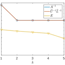
for which the bound is almost sharp: maxk(εk(E)/εk(Ub−1Lb−1)/) ≈ 9.6e+03 and µ ≈ 1.0e+04 (for k = 1). As shown in Figure 3.2, A−1 and M−1 =
b U−1
b L−1 are indeed numerically low rank, but the errorE is not.
1 2 3 4 5 10-10
10-5 100 105
Fig. 3.2: Singular value distributions ofA−1,Ub−1Lb−1, andEcorresponding to
exam-ple matrix Adefined in (3.10) for which the bound of Theorem 3.4is almost sharp. A−1and
b U−1
b
L−1are numerically low rank but the errorE is not.
Corollary 3.6. Let A = M +∆A ∈ Rn×n be nonsingular. The error E =
M−1∆Asatisfies
(3.11) εk(E)≤µβgβsεk(A−1), k≤n.
Corollary 3.6tells us that the error E retains the low-rank property ofM−1 as long asµis not too large, that is,kM−1kk∆Akis not too much larger thankM−1∆Ak, and βg and βs are not too large. Here again, inequalities (3.7) and thus (3.11) are pessimistic in practice: experiments reported in Table 3.2 show that E remains in most cases numerically low rank. These bounds should therefore not be used as a prediction of the numerical rank of E. But they do provide sufficient conditions for Eto retain low numerical rank that in some cases (e.g., the last line in Table3.2) are satisfied.
4. A novel preconditioner based on the low-rank error. Now we consider the solution of the linear system Ax=b by means of an iterative method. A clas-sical approach to accelerate the convergence of the iterative method is to use the preconditioner based on the computed LU factors
(4.1) ΠLU =Ub−1Lb−1
to solve the preconditioned systemΠLUAx=ΠLUb. However, when the LU factors have been computed at low accuracy, and when the matrixAis ill conditioned, conver-gence may still be slow. To overcome this obstacle, we propose a novel preconditioner (4.2) ΠEk= (I+Ek)
−1
b U−1Lb−1,
which is based on a rank-k approximation Ek to the error E =Ub−1Lb−1A−I. We
expect the factor (I+Ek)−1 to improve the quality of the preconditioner. In the extreme case where Ek =E, ΠE is exactly equal to A−1 and thus yields a perfect
Table 3.2: The bounds from Theorem3.4and Corollary3.6compared with the quan-tities they are bounding, using the same matrices and factorizations as in Table3.1.
matrix max k εk(E) εk(M−1) µ max k εk(E) εk(A−1) βgβsµ rotor1 (fp16) 7.6e+00 8.5e+03 7.3e+00 1.1e+13 robot (fp16) 2.1e+00 1.3e+02 2.1e+00 7.0e+07 rajat14 (fp16) 7.9e−01 2.8e+03 2.4e+00 6.0e+08 tumor 1 (fp16) 4.3e−01 4.9e+00 1.8e+00 6.9e+05 west0132 (fp16) 4.4e+00 1.6e+04 4.7e+00 3.3e+11 west0167 (fp16) 5.1e+00 6.3e+04 5.4e+00 1.6e+09 ww 36 pmec 36 (fp16) 2.0e+00 5.7e+01 4.3e+04 3.9e+10 impcol a (fp16) 2.7e−01 2.6e+01 2.7e−01 1.1e+07 impcol e (fp16) 1.4e+00 1.4e+02 1.4e+00 3.2e+03 nos1 (fp16) 5.0e+01 5.0e+05 5.9e+01 2.8e+10 steam1 (fp16) 6.1e−01 8.8e+00 6.1e−01 5.6e+11 steam3 (fp16) 4.9e−01 1.1e+03 5.1e−01 1.5e+11 randsvd(1e4,2) (fp16) 1.8e+00 2.2e+00 4.7e+02 1.1e+06 randsvd(1e7,2) (fp16) 1.8e+00 2.2e+00 1.5e+04 3.0e+10 randsvd(1e10,2) (fp16) 1.6e+00 2.1e+00 3.0e+07 1.5e+13 lund a (fp16) 2.6e+00 6.5e+00 1.2e+00 7.8e+08 lund a (ILU,τ= 10−1) 5.6e+00 1.8e+01 1.9e+01 3.7e+14 lund a (ILU,τ= 10−3) 1.1e+00 2.9e+00 6.7e+00 3.0e+06 lund a (ILU,τ= 10−5) 1.3e+00 5.4e+00 1.3e+00 1.6e+02 cavity01 (fp16) 2.3e+00 7.2e+01 2.1e+00 1.4e+09 cavity01 (ILU,τ= 10−3) 1.8e+00 4.0e+00 2.2e+00 4.1e+03 cavity01 (BLR,τ= 10−2) 5.2e−01 1.3e+02 3.2e+00 3.3e+05 cavity01 (BLR,τ= 10−3) 7.1e+00 1.3e+01 7.1e+00 1.7e+01
preconditioner, but this is obviously too expensive. However, ifknthen the solve withI+Ekcan be cheaply done with the Sherman–Morrison–Woodbury formula [16]. Since we have shown thatEis often numerically low rank, we may expectΠEk, with
some suitable smallk, to be almost as good a preconditioner asΠE. We note that the idea behind the ΠEk preconditioner shares some similarities with deflation-type
preconditioners [28], though there are fundamental differences between the two types. 4.1. Computing Ek, a low-rank approximation to E. It would be too expensive to computeEk explicitly, so we develop a matrix-free approach to its use, in which we only need to perform matrix-vector products withEk.
Although other methods could be considered, we use the randomized sampling algorithm [15], [21] which has been shown to be efficient for computing low-rank approximations to dense matrices [23]. We build Ek as a truncated SVD ofE. We consider two versions of the randomized SVD algorithm, described in Algorithms4.1
and4.2.
Both algorithms begin by sampling the columns of E with a random matrixΩ of size n×(k+p), where pis a small integer parameter that provides oversampling. A small amount of oversampling is usually enough to ensure a good accuracy of the low-rank approximation [15]. We then build an orthonormal basisV ofS; note that V captures the range ofE: E≈V VTE. In Algorithm4.1, based on this observation, we compute a rank-k approximation of VTE by means of a deterministic truncated SVD XkΣkYkT, which then yields the truncated SVD of the original matrix E as
Ek = (V Xk)ΣkYkT. This however requires us to form the product VTE which, as analyzed in the next section, can be expensive. To overcome this issue, Algorithm4.2
Algorithm 4.1 Randomized SVD algorithm from [15, Alg. 5.1] via direct SVD of VTE.
Input: matrixA, its computed LU factorsLbUb, and ann×(k+p) random matrixΩ.
1 Sample E: S =EΩ =Ub−1 Lb−1(AΩ) −Ω. 2 Orthonormalize S: V = qr(S). 3 Form VTE= (VT b U−1) b L−1
A−VT and compute an SVDVTE =XΣYT.
4 TruncateX,Σ,Y into Xk,Σk, Yk to keep onlyksingular vectors/values.
5 An SVD of Ek is given by (V Xk)ΣkYkT.
Algorithm 4.2 Randomized SVD algorithm from [15, Alg. 5.2] via row extraction. Input: matrixA, its computed LU factorsLbUb, and ann×(k+p) random matrixΩ.
1 Sample E: S =EΩ =Ub−1 Lb−1(AΩ)
−Ω.
2 Orthonormalize S: V = qr(S).
3 Compute the interpolative decomposition V = (I` W)TV(L,:).
4 ExtractE(L,:) and compute a QR factorizationE(L,:)T =QR.
5 Form (I` W)TRT and compute an SVD (I` W)TRT =XΣYT.
6 TruncateX,Σ,Y into Xk,Σk, Yk to keep onlyksingular vectors/values.
7 An SVD of Ek is given byXkΣk(QYk)T.
builds instead an interpolative decomposition (ID) [8] ofV: V = (I` W)TV(L,:),
whereI`denotes the identity matrix of order`=k+pandV(L,:)is a subset of`rows ofV. Such a decomposition can be computed by means of a pivoted QR factorization VTP =QRand by defining W =R−1:`,1:`1 R:,`+1:n andV(L,:) =P:,1:`T V [15]. We then have, definingEb=V VTE,
(4.3) E≈Eb=V V
T
E= (I` W)TV(L,:)VTE= (I` W)TEb(L,:)≈(I` W)TE(L,:). Therefore, we can build the truncated SVD ofEbased on that of (I` W)TE(L,:). The second approximation in (4.3) makes Algorithm4.2less accurate than Algorithm4.1
by a factor up to 1 +p1 + 4k(n−k) [15, Lem. 5.1]. To maintain a unified presenta-tion, we have formulated Algorithm4.2working on the orthonormal basisV. However, as explained in [15], for this second algorithm it is not necessary to orthonormalize the sample, i.e., we can work onS rather thanV. This is what we will do in practice. 4.2. The four variants of theΠEk preconditioner. In the rest of this article,
we will analyze four distinct variants ofΠEk, which differ in howEk is computed:
• ΠE(1)
k: computeEkwith Algorithm4.1and withΩa random Gaussian matrix;
• ΠE(2)
k: computeEk with Algorithm4.1and with Ωan SRFT matrix;
• ΠE(3)
k: computeEkwith Algorithm4.2and withΩa random Gaussian matrix;
• ΠE(4)
k: computeEk with Algorithm4.2and with Ωan SRFT matrix.
An SRFT matrix is a subsampled random Fourier transform matrix, defined as Ω=F R,
where F ∈ Cn×n is the discrete Fourier transform (DFT) matrix and R ∈
Rn×` is
a matrix that randomly selects ` distinct columns of F, i.e., it consists of ` random distinct columns of then×nidentity matrix.
The cost of the ΠEk preconditioner strongly depends on which variant is used.
Indeed, ΠE(1)
k requires us to perform the products EΩ and V
TE. Π(2)
Ek reduces the
cost of theEΩ product by using a SRFT matrixΩinstead. On the other hand,ΠE(3)
k
avoids forming VTE explicitly as explained in the previous section. Finally, Π(4) Ek
combines both cost reductions.
The four variants of the ΠEk preconditioner are thus decreasingly expensive.
However, they are also decreasingly accurate. Indeed, the theoretical properties of SRFT sampling are less well understood (e.g., how to choose the amount of oversam-pling). Perhaps of more concern, the row extraction SVD (Algorithm4.2) leads to an error that is up to a factor 1 +p1 + 4k(n−k) larger than that of Algorithm4.1[15, Lem. 5.1]. Since we are only building a preconditioner, this might not be too prob-lematic if it does not significantly increase the number of iterations. In the following section, we will therefore compare all four variants ofΠEk.
Regardless of the variant of ΠEk used, the new preconditioner might in some
cases perform more flops than the originalΠLU preconditioner if kis large or if the number of iterations is only reduced by a small quantity. Nevertheless, we still expect it to perform better for the following three reasons.
• The solve phase achieves in general a low execution rate because it uses BLAS 2 kernels (in the case of a single right-hand side). On the contrary, for the setup phase, the LU factorization is a BLAS 3 kernel, while computing Ek may also be achieved with BLAS 3 kernels (or “BLAS 2.5” if k is very small).
• The solve phase is performed at working precision, while the setup phase may be performed at lower precision. This includes the LU factorization but also the computation of Ek. The influence of uEk, the precision at which Ek is
computed, will be analyzed in the next section.
• Several applications require the solution for multiple right-hand sides. In this case, the setup overhead cost of the ΠEk preconditioner is amortized by the
necessity of performing more solves.
5. Numerical experiments with GMRES-IR. In this section, we analyze how our new ΠEk preconditioner can improve the convergence of GMRES-IR
(Al-gorithm 2.1) [5], which uses iterative refinement with the solves for the correction carried out by preconditioned GMRES. We use three precisions, as proposed in [6].
• The LU factorization ofAis computed at precisionuf, which is half precision for a full factorization or double precision when ILU and BLR are used. • The working precision is double precision for all experiments.
• The residual is computed in quadruple precision for all experiments. Com-puting the residuals in extended precision improves the forward error for ill-conditioned problems, though it has no effect on the convergence of iterative refinement [6].
We set the maximum number of iterative refinement steps to 10 and the maximum number of GMRES iterations per step of iterative refinement to 100 (hence a maxi-mum of 1000 total GMRES iterations is permitted). The GMRES stopping criterion is set to a relative tolerance of 10−8.
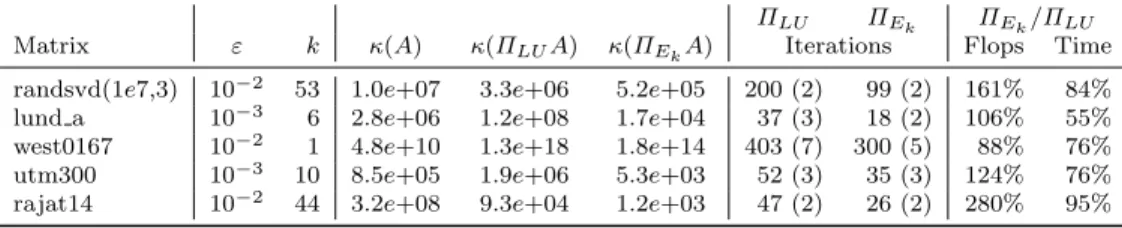
Table 5.1: Five matrices representative of typical scenarios. We used a half precision LU factorization for matrices randsvd(1e7,3) and lund a, ILU factorization withτ = 10−1 for matrices west0167 and rajat14, and BLR factorization with τ = 10−2 for matrix utm300. The seventh and eighth columns of the table show the number of GMRES iterations, with the number of iterative refinement steps in parentheses.
ΠLU ΠEk ΠEk/ΠLU
Matrix ε k κ(A) κ(ΠLUA) κ(ΠEkA) Iterations Flops Time
randsvd(1e7,3) 10−2 53 1.0e+07 3.3e+06 5.2e+05 200 (2) 99 (2) 161% 84% lund a 10−3 6 2.8e+06 1.2e+08 1.7e+04 37 (3) 18 (2) 106% 55% west0167 10−2 1 4.8e+10 1.3e+18 1.8e+14 403 (7) 300 (5) 88% 76% utm300 10−3 10 8.5e+05 1.9e+06 5.3e+03 52 (3) 35 (3) 124% 76% rajat14 10−2 44 3.2e+08 9.3e+04 1.2e+03 47 (2) 26 (2) 280% 95%
E. In our experiments, rather than setting k to a fixed value, we choose a given target accuracyε, and compute k as the numerical rank kε of E at accuracy ε (see Definition3.1).
To assess the effectiveness of each preconditioner we will measure both the number of iterations performed and the associated flops. Since our new ΠEk preconditioner
can and often does perform more flops that the traditional ΠLU preconditioner, we also estimate their run time. Since a high-performance implementation and analysis is not our focus, we use a simple model, assuming BLAS 3 computations are 10 times faster than their BLAS 2 counterparts. We also assume that computations in single and half precision are twice and four times faster than in double precision, respectively. Note that we only seek to assess the relative performance of ΠEk compared to
traditional LU-based preconditioners ΠLU. Comparing the ΠEk preconditioner to
other approaches, such as different preconditioners or direct methods, is out of the scope of this article.
5.1. Analysis of typical scenarios. In this section, we focus on the first vari-antΠE(1)
k and refer to it simply asΠEk. In Table5.1, we consider five matrices that are
representative of five typical scenarios. We report the condition numbers ofA,ΠLUA, andΠEkA. For both preconditioners, we compare the total number of GMRES
iter-ations (the number in parentheses corresponds to the number of iterative refinement steps), and the associated flops and estimated time. Note that for matrices lund a, west0167, and utm300, κ(ΠLUA) is actually higher than κ(A); nevertheless, experi-ments (not shown here) show that even on these matrices, unpreconditioned GMRES converges much slower than itsΠLU- andΠEk-preconditioned counterparts. We also
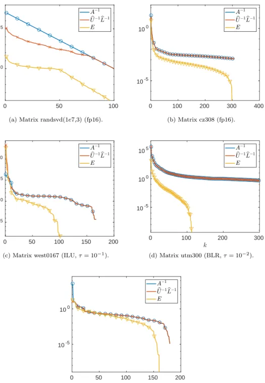
indicate the low-rank thresholdεthat we used to computeEk, and its corresponding rankk. In Figure 5.1, we plot the singular value distribution ofA−1,
b U−1
b
L−1, and
E for each of these five matrices.
We recall that our preconditioner targets ill-conditioned matrices that have a small number of small singular values and therefore a numerically low-rank inverse. Clearly, A being ill-conditioned is only a necessary condition forA−1 to be numerically low-rank, not a sufficient one. However, we have observed thatall ill-conditioned matrices that we have tested from the SuiteSparse Matrix Collection fulfill that requirement. The only matrices in our set that do not are the mode 1 and 3 randsvd matrices, which are artificially created problems. They constitute what we will call Scenario 1. In this scenario, A−1 is not numerically low rank and therefore we can expect E to have
0 50 100 100
105
(a) Matrix randsvd(1e7,3) (fp16).
0 100 200 300 400 10-5 100 (b) Matrix cz308 (fp16). 0 50 100 150 200 10-5 100 105 1010
(c) Matrix west0167 (ILU,τ= 10−1).
0 100 200 300 10-5 100 105 (d) Matrix utm300 (BLR,τ= 10−2). 0 50 100 150 200 10-5 100
(e) Matrix rajat14 (ILU,τ= 10−1).
high numerical rank and our preconditioner not to be effective. Mode 3 randsvd is analyzed in Figure5.1a. Interestingly, the SVD of the inverse factors shows a slightly faster singular value decay and therefore, even thoughA−1has high numerical rank, some improvement is observed with ΠEk over ΠLU. However, the rank k is about
n/2, leading to a significant flop overhead and thus only a modest time gain.
We emphasize that we selected the matrices based on their condition number only; we did not specifically select matrices for which A−1 is numerically low rank. While one can surely find an ill-conditioned matrix from the SuiteSparse collection that does not fulfill this requirement, we believe that the fact that one does not easily come upon one of them demonstrates that our preconditioner’s scope is very general. While A−1 is thus numerically low rank for nearly all matrices in the test set, the performance of our ΠEk preconditioner is heavily dependent on the extent to
which the error E is numerically low rank. In the following Scenarios 2, 3, and 4, E is numerically low rank and thus ΠEk performs well. We distinguish three cases
depending on the reason forEto have low numerical rank. In Scenario 2, the SVD of Eclosely follows that ofA−1(Figure5.1b); in other cases, the SVD ofEshows an even faster decay than that ofA−1, either because
b U−1
b
L−1 has lower numerical rank than
A−1(Scenario 3, Figure 5.1c), or because E has lower numerical rank than
b U−1
b L−1 (Scenario 4, Figure5.1d). Scenario 3 generally happens when the approximateLbUb
factors are nearly singular, thus leading to a very ill-conditionedΠLUA matrix. By usingΠEk, we can reduce the ill conditioning ofΠLUA. We conjecture that Scenario 4
is due to a∆Athat possesses some kind of structure, and we have in fact observed it to be especially frequent for the test cases with BLR factorization.
Finally, Scenario 5 contains the unfortunate cases for whichE loses the low-rank property of A−1 (Figure 5.1e). In our set of matrices, this is always due to
b U−1
b L−1 not being numerically low rank (i.e., the bound from Theorem 3.3 is sharp and βg or βs is large). We recall that in section3 we built a matrix for whichE loses the low-rank property due to a special∆A(see (3.10)), but this did not occur on any of the matrices of our set.
The numerical rankkε ofE at accuracyεcan be quite large for matrices falling into Scenarios 1 and 5. While the preconditioner ΠEk is not designed with these
matrices in mind, it is nevertheless desirable that, when used on such matrices, the overhead cost due to the use of ΠEk remain limited. To do so, we limit k to be no
larger than a given kmax. For example, for rajat14, using kmax = n/10, the flop
overhead cost of ΠEk is reduced from 280% to 170% of that of ΠLU, and the time
gain is increased from 95% to 92%.
This diversity of scenarios shows that the optimal choice of the preconditioner pa-rameters will be heavily matrix dependent. However, we would like to design a “black box” version of the preconditioner that has default settings for which it performs well on a wide range of problems. This is the aim of the next section.
5.2. Finding a black box setting. Three main parameters influence the cost and accuracy of the preconditionerΠEk: the precisionuEk at whichEk is computed,
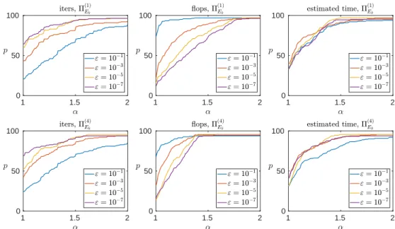
the low-rank threshold ε, and the amount of oversampling p. In this section, we analyze how to set these parameters to produce good performance on a wide range of problems. In order to do that we seek the best value for each parameter separately, using performance profiles [10], [17, sec. 26.4]. Each performance profile corresponds to a preconditioner, a selection of three or four parameters, and a chosen performance measure for which smaller is better. Each curve on a performance profile shows, for a range of values of α≥ 1, the proportion of problems p ∈ [0,1] for which the
performance measure for a particular parameter was within a factorαof the smallest performance measure over all the parameter values. The performance measures are the number of iterations, the number of flops, and the time predicted by our model.
Note that if the iteration fails to converge for some problems for a given parameter then the corresponding curve in the performance profile never reachesp= 1; thus the value ofpat which a curve levels off is a measure of robustness.
Naturally, the parameters are interdependent: for example, a high oversampling parameter will increase the weight of the sampling operation, which is performed at precision uEk, thus increasing the importance of the latter parameter. While the
approach of studying each parameter independently is thus possibly not optimal, it allows us to find a suitable setting without getting lost into the combinatorics of the parameters.
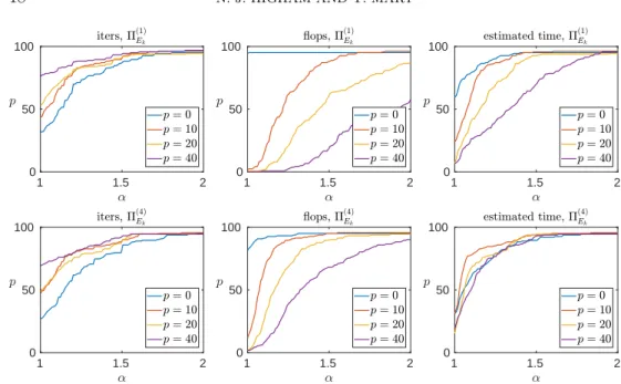
We first analyze the influence of the oversampling parameterp. From Figure5.2, it is clear that a larger oversampling leads to a greater reduction of the number of iterations, but also to a greater flop overhead due to the larger subspace size`=k+p. We must therefore find a compromise aiming at minimizing the time estimated by our model. Interestingly, the time performance profiles suggest that the value forpshould be set differently depending on which ΠEk variant is considered. Indeed, Π
(1) Ek and
ΠE(2)
k require us to form the product V
TE and their cost is thus very sensitive to the choice of p; setting it to a small value works best. Conversely, ΠE(3)
k and Π
(4) Ek
avoid forming VTE, and we can thus afford to take much higher values of p, since building the preconditioner is much cheaper. This is visible from the time plots (right column) in Figure 5.2, where the curves corresponding to small ptend to be above those corresponding to largepforΠE(1)
k (top row), while the opposite is true forΠ
(4) Ek
(bottom row). Results for ΠE(2)
k and Π
(3)
Ek variants (not shown in Figure 5.2), lie in
the middle ground. In the following, we will therefore use p= 0 forΠE(1)
k and Π (2) Ek, andp= 10 forΠE(3) k andΠ (4) Ek.
We now turn to the low-rank threshold parameter ε, whose effect is plotted in Figure 5.3. The trend is again clear: a smaller value of εmakes the preconditioner more robust but more costly. The role ofεis also strongly dependent on which variant ofΠEk is considered, for the same reasons than the oversampling parameter. In the
following, we will useε= 10−3 forΠ(1) Ek andΠ (2) Ek, and ε= 10 −5forΠ(3) Ek andΠ (4) Ek.
Finally, in Figure 5.4 we study the role of the uEk precision parameter on the
subset of tests performed with half precision LU factorization (fp16). ComputingEkin half precision leads to a preconditioner that is less accurate than whenEkis computed in higher precision: in particular, in about 8% of the cases the preconditioner fails whenEkis built in half precision, whereas it succeeds with a higher precisionuEk. On
the other hand, computingEk in single or double precision makes little difference on this set of problems, and since single precision is twice as fast as double precision, the time performance profile shows that settinguEk to single is the best strategy overall,
for all four variants ofΠEk.
5.3. Results on the full set of problems with the black box setting. In this section we report numerical experiments on the full set of problems using the black box settings chosen in the previous section, which we summarize in Table5.2.
We emphasize that the results were obtained without tuning the preconditioner parameters on a case-by-case basis, thereby demonstrating the generality and versa-tility of the preconditioner.
1 1.5 2 0 50 100 1 1.5 2 0 50 100 1 1.5 2 0 50 100 1 1.5 2 0 50 100 1 1.5 2 0 50 100 1 1.5 2 0 50 100
Fig. 5.2: Performance profile of the ΠEk preconditioner for different oversampling
parametersp. The other parameters were set toε= 10−5 andu
Ek = single.
Table 5.2: Black box settings devised in section5.2.
ε p uEk ΠE(1) k 10 −3 0 single ΠE(2) k 10 −3 0 single ΠE(3) k 10 −5 10 single ΠE(4) k 10 −5 10 single
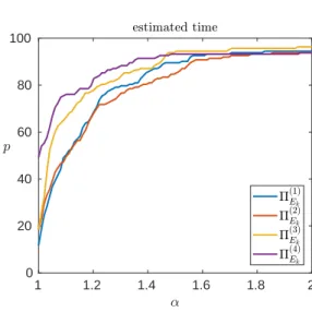
We first compare the four variants of theΠEkpreconditioner. Figure5.5shows the
time performance profile of each variant. Note that we do not provide the iterations and flop profiles, since comparing the four variants in terms of iterations or flops is not meaningful, because they are used with different values of εand/orp. We must compare their time performance to assess which variant finds the best cost/accuracy compromise. The preconditionerΠE(4)
k ranks first on the largest number of problems
(about 50% of them); it is, however, less robust than the other variants, failing to converge in three cases where the other variants converged. We therefore choose to reject it. While ΠE(1)
k and Π
(2)
Ek are significantly slower, Π
(3)
Ek achieves a good
performance overall, very close to that of ΠE(4)
k. Interestingly, it is also the most
robust variant; recalling that it is less accurate than ΠE(1)
k by a factor up to 1 +
p
1 + 4k(n−k), this means that it compensates its lesser accuracy by being able to afford a much smaller threshold (ε= 10−5 instead of 10−3). We conclude that Π(3) Ek
1 1.5 2 0 50 100 1 1.5 2 0 50 100 1 1.5 2 0 50 100 1 1.5 2 0 50 100 1 1.5 2 0 50 100 1 1.5 2 0 50 100
Fig. 5.3: Performance profile of theΠEk preconditioner for different low-rank
thresh-oldεparameters. The other parameters were fixed top= 10 anduEk= single.
1 1.5 2 0 50 100 1 1.5 2 0 50 100 1 1.5 2 0 50 100
Fig. 5.4: Performance profile of theΠE(1)
k preconditioner for an LU factorization
com-puted in half precision for different uEk precision parameters, with ε = 10
−5 and
p= 10. Results withΠE(2,3,4)
k are similar.
is the choice that leads to the best performance overall on this set of problems. We now compareΠE(3)
k with the classical ΠLU preconditioner. In Figure 5.6, we
plot the relative performance ofΠE(3)
k with respect toΠLU. Each bar corresponds to
a different test case, its color indicating which type of approximate factorization is considered (fp16, ILU, or BLR). The colors are evenly distributed, which means that the numerical behavior ofΠE(3)
k is comparable for all three types of factorization. The
preconditionerΠE(3)
k leads to a lower number of iterations thanΠLU in about 80% of
the test cases. Moreover, this reduction of the number of iterations is often significant: ΠLU performs more than 50% more iterations on 30% of the test cases. Interestingly,
1 1.2 1.4 1.6 1.8 2 0 20 40 60 80 100
Fig. 5.5: Time performance profile of the four variants of the ΠEk preconditioner,
obtained with the black box settings described in Table5.2.
in about 5% of the cases,ΠLU fails to converge whereasΠ (3)
Ek successfully solves the
problem (indicated by the white gap on the left side of the plots). Therefore, even thoughΠE(3)
k leads to a flop overhead compared withΠLU in about 90% of the cases,
that overhead is often limited (less than 50% overhead in half the cases) and using our simple performance model, the estimated time results suggest significant gains can be expected.
5.4. Results on larger matrices. In this section we complement the previous results with some experiments on larger matrices. These experiments include only the ILU and BLR preconditioners because the fp16 arithmetic we are using is too slow on matrices of size larger than 1000. An important question is whether these larger matrices still possess an inverse that is numerically low rank, and whether the numerical rankkεofA−1remains small or increases withn.
Table5.3shows results for some matrices of size around 5000 from the SuiteSparse collection. We see that theΠEk preconditioner significantly improves the number of
iterations for both the ILU and BLR preconditioners. Importantly, this improve-ment is achieved for very small ranks (kε remains smaller than 100 for all matrices) compared with the matrix sizesn.
In Figure5.7we comparekεfor different matrix sizes for two families of matrices (also from the SuiteSparse Matrix Collection) that contain cz308 and utm300 in Ta-ble2.1. The plots show that the numerical rank remains almost constant with respect ton when the requiredεis not too small. While there may of course be some other matrices for which this property is not true, the figure suggests that, at least for some problem classes, our preconditioner should perform well, or even better, on large-scale problems.
6. Conclusion. We have presented a new and very general preconditioner for iterative methods for solving ill-conditioned linear systemsAx=b.
The key idea is to exploit the low numerical rank structure that is typically present in the error arising in approximate matrix factorizations. We have defined a general
20 40 60 80 100 120 140 160 0 0.5 1 1.5 2 20 40 60 80 100 120 140 160 0 1 2 3 20 40 60 80 100 120 140 160 0 0.5 1 1.5 2 2.5
Fig. 5.6: Performance comparison between theΠLU preconditioner and the best vari-ant of the ΠEk preconditioner (Π
(3)
Ek). Each bar corresponds to one of the 163 test
cases, its color indicating which type of approximate factorization is considered (fp16, ILU, or BLR). The y-axis corresponds to the normalized performance of ΠEk with
respect to that ofΠLU: thus,ΠEk performs better thanΠLU when the bar is under
the black line. These results were obtained with the black box settings described in Table 5.2. The white gap on the left side of the plots corresponds to the test cases for whichΠLU did not converge whereasΠEk did.
Table 5.3: Results on larger matrices. The last two columns of the table show the number of GMRES iterations, with the number of iterative refinement steps in paren-theses.
Iterations Matrix Application n κ(A) Fact. type ε kε ΠLU ΠEk
msc04515 Structural 4515 2.3e+06 ILU (τ= 10
−4) 10−1 17 41(2) 31(2) BLR (τ= 10−2) 10−3 7 30(2) 24(2) gemat12 Power Network 4929 1.0e+08 ILU (τ= 10
−5) 10−3 42 16(2) 9(2) BLR (τ= 10−3) 10−3 59 24(2) 14(2) c-24 Optimization 4119 2.2e+08 BLR (τ= 10 −4) 10−2 56 9(2) 7(2) BLR (τ= 10−3) 10−3 98 29(3) 15(3) lhr04c Chemical 4101 3.8e+12 ILU (τ= 10 −7) 10−5 16 30(3) 12(3) BLR (τ= 10−5) 10−4 14 40(3) 24(3)
10-7 10-5 10-3 10-1 100 101 102 103 104 10-7 10-5 10-3 10-1 100 101 102 103 104
Fig. 5.7: Numerical rank kε of A−1 at accuracy ε for different matrix sizes. The matrices are from the SuiteSparse Matrix Collection and the digits in the name denote the matrix size.
framework in which a low accuracy LU factorizationA=LbUb+∆Ais computed. This
allows for many different types of approximate LU factorizations, among which in our experiments we have used half precision LU, incomplete LU, and block low-rank LU. We have used theoretical results from singular value perturbation analysis to bound the distance fromE=Ub−1Lb−1A−I=Ub−1Lb−1∆Ato a numerically low-rank
matrix by a multiple of the distance from A−1 to a numerically low-rank matrix. These bounds give sufficient conditions for the error matrix to be numerically low rank. In practice, the bounds are generally pessimistic and we have found E to be almost always numerically low rank in practice whenAis ill conditioned.
Our novel preconditioner improves the traditional preconditionerUb−1Lb−1based
on the approximate LU factors by premultiplying it by a correction term (I+Ek)−1, exploiting the numerical low rank ofE. Because building E explicitly is too expen-sive, our algorithm uses a matrix-free approach based on randomized sampling to compute a rank-kmatrixEk as a truncated SVD ofE. We have compared four vari-ants of the algorithm theoretically, by performing a computational cost analysis, and experimentally.
After experimenting with the internal parameters of the preconditioner, in or-der to better unor-derstand its practical behavior, we chose a set of parameters that we applied in a black box manner to a large set of real-life problems coming from a variety of applications. Our numerical results show the capacity of the new precondi-tioner to accelerate the solution of a wide range of ill-conditioned problems, thereby demonstrating its generality and versatility.
We conclude by mentioning some possible directions for future work. Our pre-conditioner could be coupled with other iterative methods than GMRES-IR, such as GMRES. The LU framework that we have described could also be naturally adapted to symmetric problems. We believe our work could even be extended to precondi-tioners that are not based on matrix factorizations, such as Jacobi, Gauss-Seidel, approximate inverse, or multigrid approaches.
Most importantly, while out of the scope of this article, a high-performance im-plementation of the proposed preconditioner will be of interest both to assess the performance gains that can be achieved and to study its numerical behavior on
large-scale problems.
Acknowledgements. We thank Patrick R. Amestoy and Alfredo Buttari for useful discussions and the referees for helpful suggestions.
REFERENCES
[1] P. Amestoy, C. Ashcraft, O. Boiteau, A. Buttari, J.-Y. L’Excellent, and C. Weis-becker,Improving multifrontal methods by means of block low-rank representations, SIAM J. Sci. Comput., 37 (2015), pp. A1451–A1474,https://doi.org/10.1137/120903476. [2] P. Amestoy, A. Buttari, J.-Y. L’Excellent, and T. Mary,On the complexity of the block
low-rank multifrontal factorization, SIAM J. Sci. Comput., 39 (2017), pp. A1710–A1740, https://doi.org/10.1137/16M1077192.
[3] P. R. Amestoy, A. Buttari, J.-Y. L’Excellent, and T. Mary,Performance and scalability of the block low-rank multifrontal factorization on multicore architectures, ACM Trans. Math. Software, (2017). Submitted.
[4] M. Bebendorf,Hierarchical Matrices: A Means to Efficiently Solve Elliptic Boundary Value Problems, vol. 63 of Lecture Notes in Computational Science and Engineering, Springer-Verlag, Berlin, 2008,https://doi.org/10.1007/978-3-540-77147-0.
[5] E. Carson and N. J. Higham,A new analysis of iterative refinement and its application to accurate solution of ill-conditioned sparse linear systems, SIAM J. Sci. Comput., 39 (2017), pp. A2834–A2856,https://doi.org/10.1137/17M1122918.
[6] E. Carson and N. J. Higham, Accelerating the solution of linear systems by iterative re-finement in three precisions, SIAM J. Sci. Comput., 40 (2018), pp. A817–A847, https: //doi.org/10.1137/17M1140819.
[7] T. F. Chan and D. E. Foulser, Effectively well-conditioned linear systems, SIAM J. Sci. Statist. Comput., 9 (1988), pp. 963–969,https://doi.org/10.1137/0909067.
[8] H. Cheng, Z. Gimbutas, P. G. Martinsson, and V. Rokhlin,On the compression of low rank matrices, SIAM J. Sci. Comput., 26 (2005), pp. 1389–1404,https://doi.org/10.1137/ 030602678.
[9] T. A. Davis and Y. Hu,The University of Florida Sparse Matrix Collection, ACM Trans. Math. Software, 38 (2011), pp. 1:1–1:25,https://doi.org/10.1145/2049662.2049663. [10] E. D. Dolan and J. J. Mor´e,Benchmarking optimization software with performance profiles,
Math. Programming, 91 (2002), pp. 201–213,https://doi.org/10.1007/s101070100263. [11] C. Eckart and G. Young,The approximation of one matrix by another of lower rank,
Psy-chometrika, 1 (1936), pp. 211–218,https://doi.org/https://doi.org/10.1007/BF02288367. [12] J. A. George,Nested dissection of a regular finite-element mesh, SIAM J. Numer. Anal., 10
(1973), pp. 345–363,https://doi.org/10.1137/0710032.
[13] A. Haidar, S. Tomov, J. Dongarra, and N. J. Higham, Harnessing GPU tensor cores for fast FP16 arithmetic to speed up mixed-precision iterative refinement solvers, 2018. Submitted to Supercomputing 2018.
[14] A. Haidar, P. Wu, S. Tomov, and J. Dongarra, Investigating half precision arithmetic to accelerate dense linear system solvers, in Proceedings of the 8th Workshop on Latest Advances in Scalable Algorithms for Large-Scale Systems, ScalA ’17, Nov. 2017, pp. 10:1– 10:8,https://doi.org/10.1145/3148226.3148237.
[15] N. Halko, P. G. Martinsson, and J. A. Tropp,Finding structure with randomness: Prob-abilistic algorithms for constructing approximate matrix decompositions, SIAM Rev., 53 (2011), pp. 217–288,https://doi.org/10.1137/090771806.
[16] H. V. Henderson and S. R. Searle,On deriving the inverse of a sum of matrices, SIAM Rev., 23 (1981), pp. 53–60,https://doi.org/10.1137/1023004.
[17] D. J. Higham and N. J. Higham,MATLAB Guide, Society for Industrial and Applied Math-ematics, Philadelphia, PA, USA, third ed., 2017.
[18] N. J. Higham,Optimization by direct search in matrix computations, SIAM J. Matrix Anal. Appl., 14 (1993), pp. 317–333,https://doi.org/10.1137/0614023.
[19] R. A. Horn and C. R. Johnson, Topics in Matrix Analysis, Cambridge University Press, Cambridge, UK, 1991,https://doi.org/https://doi.org/10.1137/1035037.
[20] R. A. Horn and C. R. Johnson,Matrix Analysis, Cambridge University Press, Cambridge, UK, second ed., 2013,https://doi.org/https://doi.org/10.1137/1030034.
[21] E. Liberty, F. Woolfe, P.-G. Martinsson, V. Rokhlin, and M. Tygert,Randomized algo-rithms for the low-rank approximation of matrices, Proceedings of the National Academy of Sciences, 104 (2007), pp. 20167–20172,https://doi.org/10.1073/pnas.0709640104.
[22] T. Mary,Block Low-Rank Multifrontal Solvers: Complexity, Performance, and Scalability, PhD thesis, Universit´e de Toulouse, Toulouse, France, Nov. 2017,http://personalpages. manchester.ac.uk/staff/theo.mary/doc/thesis.pdf.
[23] T. Mary, I. Yamazaki, J. Kurzak, P. Luszczek, S. Tomov, and J. Dongarra,Performance of random sampling for computing low-rank approximations of a dense matrix on GPUs, in Proceedings of the International Conference for High Performance Computing, Networking, Storage and Analysis, SC ’15, New York, NY, USA, 2015, ACM, pp. 60:1–60:11,https: //doi.org/10.1145/2807591.2807613.
[24] L. Mirsky, Symmetric gauge functions and unitarily invariant norms, Quart. J. Math., 11 (1960), pp. 50–59,https://doi.org/10.1093/qmath/11.1.50.
[25] C. B. Moler, Cleve Laboratory. http://mathworks.com/matlabcentral/fileexchange/ 59085-cleve-laboratory.
[26] Multiprecision Computing Toolbox. Advanpix, Tokyo.http://www.advanpix.com.
[27] Y. Saad, Iterative Methods for Sparse Linear Systems, Society for Industrial and Ap-plied Mathematics, Philadelphia, PA, USA, second ed., 2003, https://doi.org/10.1137/ 1.9780898718003.
[28] J. M. Tang, R. Nabben, C. Vuik, and Y. A. Erlangga,Comparison of two-level precon-ditioners derived from deflation, domain decomposition and multigrid methods, SIAM J. Sci. Comput., 39 (2009), pp. 340–370,https://doi.org/10.1007/s10915-009-9272-6.