Some Contributions to Nonparametric Estimation of Density and Related Functionals for Biased Data

S

OME

C

ONTRIBUTIONS TO

N

ONPARAMETRIC

E

STIMATION OF

D

ENSITY AND

R

ELATED

F

UNCTIONALS FOR

B

IASED

D

ATA

J

L

A THESIS

IN THE

D

OF

MATHEMATICS AND

STATISTICS

P

P

F

R

FOR THE

DEGREE OF

DOCTOR OF

PHILOSOPHY AT

C

U

M

Q

C

SEPTEMBER

2010

c

Abstract

Some Contributions to Nonparametric Estimation of Density

and Related Functionals for Biased Data

Jun Li, Ph.D.

Concordia University, 2010

Length biased sampling, as a special case of general biased sampling, occurs naturally in many statistical applications. In problems related with such applications, two different density functions are involved. One of them is the density of interest, which is referred to as the unweighted density, information about which is not observable directly in prac-tice; the other one is referred to as the weighted density, the sample from which could be observed directly. These two densities are connected through a weight function. One aspect regarding data from weighted density is to estimate the unweighted density from the sample obtained using the weighted density. In this thesis we concentrate on the weight function representing length of the sampling unit that results in a sample called length-biased sample. Since most of such data are nonnegative, unweighted density has a non-negative support where common kernel density estimators with symmetric kernel may not be appropriate. Such density estimators usually generate the edge effect, which makes these to have large bias at the lower boundary. One possible reason for this is that symmetric kernels may assign some weights in region of zero probability.

In this thesis, we propose some new smooth density estimators based on Poisson distribution and nonnegative asymmetric kernels for length biased data to take care of

the edge effect. We investigate asymptotic behavior of these proposed density estimators as well as their finite sample performance through extensive simulation studies, that is more meaningful in practice. Also, we compare our new density estimators with other estimators in literature. Further, in addition to density estimators, we also consider smooth estimators of distribution function and some other functionals of the density such as hazard function and mean residual life function.

Acknowledgements

I would like to express my sincere gratitude to my supervisor Dr. Yogendra P. Chaubey, for his kindness, constructive suggestions on my thesis and useful help in the completion of this dissertation.

I would also like to accord my heartfelt gratefulness to my teachers for their instruction and direct or indirect help during my studies at Concordia.

Last but not the least I would like to express my deep appreciation to my beloved par-ents and my dear wife for their understanding, encouragement and consistent support without which I may not be able to complete this difficult task.

Contents

List of Tables xiii

List of Figure xvi

List of Acronyms xvii

List of Symbols xviii

1 Introduction 1

1.1 Biased and Length Biased Data . . . 1

1.2 Nonparametric Functional Estimation for Biased Data . . . 4

1.3 Motivation of the Estimators . . . 11

1.4 Objectives . . . 12

1.5 Organization of the Thesis . . . 13

2 Smooth Estimators of Density and Distribution Functions Based on Cox’s Estimator 14 2.1 Introduction . . . 14

2.2 Estimators of Distribution and Density Functions with Poisson Weights 15 2.2.1 Smooth Estimator of Cumulative Distribution Function . . . 15

2.2.2 Smooth Density Estimator . . . 19

2.2.2.1 Asymptotic Properties of ˜fn(x) . . . 20

2.2.2.2 Proof of Theorems . . . 21

2.3 Estimators of Distribution and Density Functions with Asymmetric Ker-nels . . . 28

2.3.1 Smooth Estimator of Distribution Function with Asymmetric Ker-nels . . . 28

2.3.1.1 Asymptotic Properties . . . 28

2.3.1.2 MSE . . . 32

2.3.2 Density Estimator using Asymmetric Kernels . . . 32

2.3.2.1 Asymptotic property of ˜f+ n(x) . . . 33

2.3.2.2 AMISE . . . 37

2.3.3 Corrected Density Estimator . . . 39

2.4 Other Density Estimators with Asymmetric Kernels . . . 40

2.4.1 Chen Density Estimators for Length Biased Data . . . 40

2.4.2 Scaillet Density Estimators for Length Biased Data . . . 41

3 Smooth Estimators of Density and Distribution Functions Based on Empirical Distribution Function 43 3.1 Introduction . . . 43

3.2 Estimators of Density and Distribution Functions with Poisson Weights 45 3.2.1 Smooth Density Estimator . . . 45

3.2.1.1 Asymptotic Property of ˆfn(x) . . . 46

3.2.2 Distribution Function Estimator . . . 51

3.3 Estimators of Density and Distribution Functions with Asymmetric Ker-nel . . . 56

3.3.1 Smooth Density Estimator . . . 56

3.3.1.1 Asymptotic Properties . . . 57

3.3.1.2 MSE and AMISE . . . 59

3.3.1.3 Corrected Density Estimator . . . 60

3.3.2 Smooth Estimator of Distribution Function . . . 61

4 A Numerical Study of the New Estimators 65 4.1 Introduction . . . 65

4.2 A Comparison of Different Criteria for Selecting Smoothing Parameters: The Case of ˜fn . . . 67

4.2.1 Unbiased Cross-Validation Method . . . 68

4.2.1.1 Kullback-Liebler Divergence Cross Validation . . . 68

4.2.1.2 Integrated Squared Error Cross Validation . . . 69

4.2.1.3 Hellinger Distance . . . 70

4.2.1.4 Simulation Studies for Optimal Smoothing Parameter: The Case of ˜fn . . . 70

4.2.2 Biased Cross-Validation Method . . . 83

4.2.2.1 Simulation Studies . . . 84

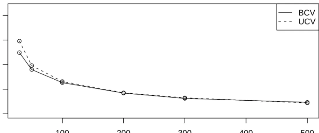
4.2.3 Choice Between UCV and BCV Methods . . . 95

4.3 Parameter Selection for Other Density Estimators . . . 97

4.3.1 Parameter Selection for ˜f+ n(x) and ˜fn∗(x) . . . 97

4.3.1.1 Biased Cross-Validation . . . 98

4.3.1.2 Unbiased Cross-Validation . . . 98

4.3.1.3 Numerical Comparison . . . 99

4.3.2 Parameter Selection for ˜f∗ n(x) . . . 103

4.3.3 Parameter Selection for ˆfn(x) . . . 103

4.3.4 Parameter Selection for ˆf+ n(x) and ˆfn∗(x) . . . 104

4.3.5 Parameter Selection for Chen and Scaillet Estimators . . . 104

4.4 A Comparison Between Different Estimators: Simulation Studies . . . . 105

4.4.1 Simulation for χ2 2 and χ26 . . . 105

4.4.2 Simulation for Some Other Standard Distributions . . . 115

4.4.3 Discussions and Conclusions . . . 128

4.5 A Linear Combination of Two Density Estimators . . . 131

5 Smooth Estimators of Some Functionals of the Distribution Function140 5.1 Introduction . . . 140

5.2 Smooth Estimators of Hazard Function . . . 141

5.2.1 Estimators with Poisson Weights . . . 141

5.2.1.1 Asymptotic Property of Hen(x) and ˜hn(x) . . . 142

5.2.1.2 MSE . . . 144

5.2.2 Estimator with Asymmetric Kernels . . . 144

5.2.2.1 Asymptotic Properties of ˜h∗ n(x) . . . 145

5.2.2.2 MSE . . . 145

5.2.3 Numerical Comparison . . . 146

5.3.1 Smooth Estimator of MRL with Poisson Weights Based on Fn . 152

5.3.2 Smooth Estimator of MRL with Poisson Weights Based on Gn . 158

5.3.3 Smooth Estimator of MRL with Asymmetric Kernels . . . 163

5.3.4 Numerical Comparison . . . 166

6 Future Research 173 6.1 Dependent Data . . . 173

6.2 Censored Data . . . 174

6.3 Unknown Weight Function . . . 176

6.4 Estimation of Other Functionals and Their Integrals . . . 177

List of Tables

4.1 Parameter and ISE . . . 96

4.2 Simulated MISE forχ2 2 . . . 106

4.3 Simulated MSE for χ2 2 . . . 107

4.4 Simulated MSE for χ2 2 . . . 108

4.5 Simulated MSE for χ2 2 . . . 109

4.6 Simulated MISE forχ2 6 . . . 110

4.7 Simulated MSE for χ2 6 . . . 111

4.8 Simulated MSE for χ2 6 . . . 112

4.9 Simulated MSE for χ2 6 . . . 113

4.10 Simulated MISE for Lognormal withµ= 0 . . . 116

4.11 Simulated MSE for Lognormal withµ= 0 . . . 117

4.12 Simulated MSE for Lognormal withµ= 0 . . . 118

4.13 Simulated MSE for Lognormal withµ= 0 . . . 119

4.14 Simulated MISE for Weibull with α= 2 . . . 120

4.15 Simulated MSE for Weibull withα = 2 . . . 121

4.16 Simulated MSE for Weibull withα = 2 . . . 122

4.18 Simulated MSE for Mixture of Two Exponential Distributions with π=

0.4,θ1 = 2 and θ2 = 1 . . . 124

4.19 Simulated MSE for Mixtures of Two Exponential Distributions withπ= 0.4,θ1 = 2 and θ2 = 1 . . . 125

4.20 Simulated MSE for Mixtures of Two Exponential Distributions withπ= 0.4,θ1 = 2 and θ2 = 1 . . . 126

4.21 Simulated MSE for Mixtures of Two Exponential Distributions withπ= 0.4,θ1 = 2 and θ2 = 1 . . . 127

4.22 Simulated MISE for Standard Distributions . . . 133

4.23 Simulated MSE for χ2 2 Distribution . . . 134

4.24 Simulated MSE for χ2 6 Distribution . . . 135

4.25 Simulated MSE for Lognormal Distribution . . . 136

4.26 Simulated MSE for Weibull Distribution . . . 137

4.27 Simulated MSE for Mixtures of Two Exponential Distributions withπ= 0.4,θ1 = 2 and θ2 = 1 . . . 138

5.1 Simulated MSE for χ2 2 . . . 147

5.2 Simulated MSE for χ2 6 . . . 148

5.3 Simulated MSE for Lognormal(0,1) . . . 149

5.4 Simulated MSE for Γ(2,1) . . . 150

5.5 Simulated MSE for Weibull(4) . . . 151

5.6 Simulated MSE for χ2 2 . . . 168

5.7 Simulated MSE for χ2 6 . . . 169

5.9 Simulated MSE for Lognormal(0) . . . 171 5.10 Simulated MSE for Weibull(4) . . . 172

List of Figures

1.1 Plots of density function of χ2

12 and its Bhattacharyya et al. kernel

estimator. Solid line represents true density and dash line represents the estimator. . . 7 1.2 Plots of density function ofχ2

2and its Jones kernel estimator with Normal

kernel. Solid line represents true density and dash line represents the estimator. . . 8

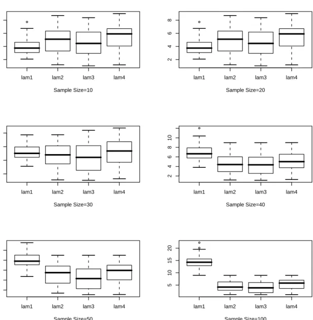
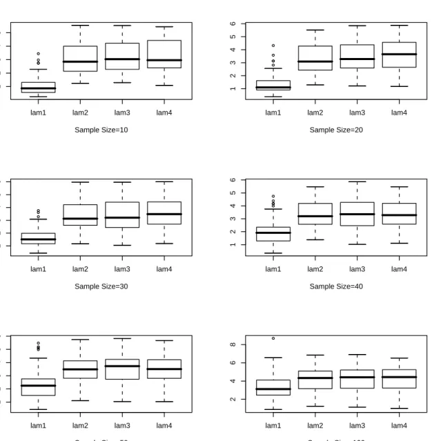
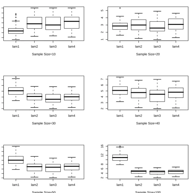
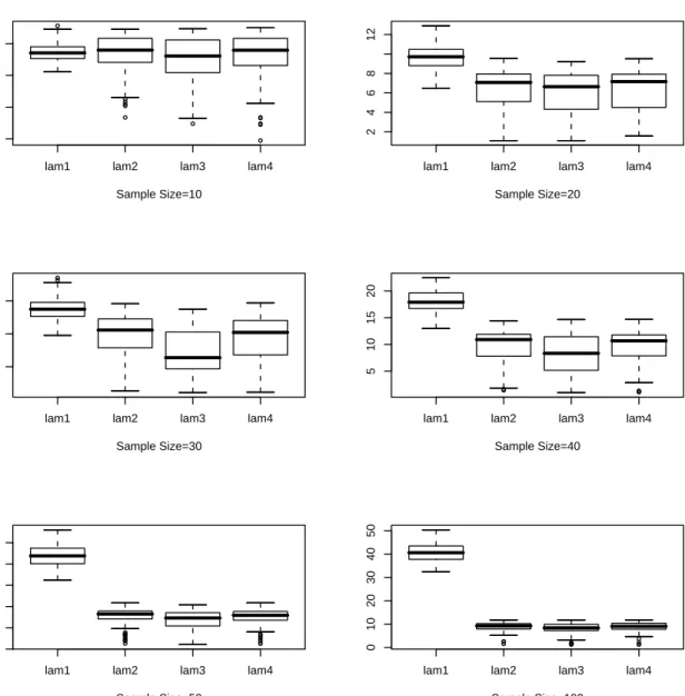
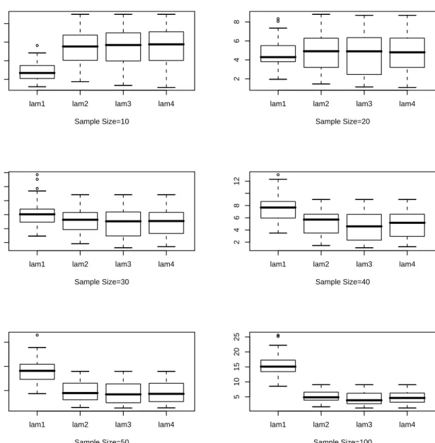
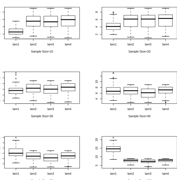
4.1 CV(λ) Plots, Sample Size=100 . . . 72 4.2 Smooth Density Plots, Sample Size=100 . . . 73 4.3 Box Plot forλnfor 100 Samples, Underlying Density: Exponential, lam1:

For Chaubey-Sen Choice, lam2: KL Cross Validation, lam3: ISE Cross Validation, lam4: Optimum Hellinger Distance . . . 76 4.4 Box Plot for for λn for 100 Samples, Underlying Density: Lognormal,

lam1: For Chaubey-Sen Choice, lam2: KL Cross Validation, lam3: ISE Cross Validation, lam4: Optimum Hellinger Distance . . . 77 4.5 Box Plot for for λn for 100 Samples, Underlying Density: Gamma(2,1),

lam1: For Chaubey-Sen Choice, lam2: KL Cross Validation, lam3: ISE Cross Validation, lam4: Optimum Hellinger Distance . . . 78

4.6 Box Plot for forλnfor 100 Samples, Underlying Density: Weibull,α = 2,

, lam1: For Chaubey-Sen Choice, lam2: KL Cross Validation, lam3: ISE

Cross Validation, lam4: Optimum Hellinger Distance . . . 79

4.7 Box Plot for for λn for 100 Samples, Underlying Density: Exponential Mixture, θ1 = 2, θ2 = 1, π = 0.4, lam1: For Chaubey-Sen Choice, lam2: KL Cross Validation, lam3: ISE Cross Validation, lam4: Optimum Hellinger Distance . . . 80

4.8 Box Plot for for λn for 100 Samples, Underlying Density: Exponential Mixture, θ1 = 10, θ2 = 1, π = 0.2, lam1: For Chaubey-Sen Choice, lam2: KL Cross Validation, lam3: ISE Cross Validation, lam4: Optimum Hellinger Distance . . . 81

4.9 Boxplots of parameter and ISE for χ2 2. . . 86

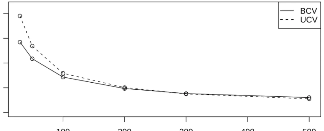
4.10 Plots of BCV and UCV MISE forχ2 2. . . 86

4.11 Boxplots of parameter and ISE for χ2 6. . . 88

4.12 Plots of BCV and UCV MISE forχ2 6. . . 88

4.13 Boxplots of parameter and ISE for Lognormal with parameter 1. . . 90

4.14 Plots of BCV and UCV MISE for Lognormal with parameter 1. . . 90

4.15 Boxplots of parameter and ISE for Weibull with parameter 2. . . 92

4.16 Plots of BCV and UCV MISE for Weibull with parameter 2. . . 92

4.17 Boxplots of parameter and ISE for mixtures of two exponential distribu-tions, π= 0.4,θ1 = 2, θ2 = 1. . . 94

4.18 Plots of BCV and UCV MISE for mixtures of two exponential distribu-tions, π= 0.4,θ1 = 2, θ2 = 1. . . 94

4.19 UCV function forχ2 6, sample size=100. . . 95

4.20 BCV function for χ2

6, sample size=100. . . 96

4.21 Density and estimators forχ3

6. . . 96

4.22 Plots of samples of (v2

n, εn) and ISE for χ22. . . 100

4.23 Plots of samples of (v2

n, εn) and ISE for χ26.. . . 101

4.24 Plot of MISE forχ2

2. . . 102

4.25 Plot of MISE forχ2

6. . . 102

List of Acronyms

AMISE Asymptotic Mean Integrated Square Error AIV Asymptotic Integrated Variance

BCV Biased Cross-Validation

CDF Cumulative Distribution Function CV Cross-Validation

i.i.d. independent and identically distributed ISE Integrated Squared Error

LB Length Biased

MISE Mean Integrated Squared Error MRL Mean Residual Life

MSE Mean Squared Error

NPMLE Nonparametric Maximum Likelihood Estimator PDF Probability Density Function

PWE Poisson Weights Estimator UCV Unbiased Cross-Validation

List of Symbols

χ2

α Chi-Square Function with Parameter α a.s.

−→ Convergence Almost Surely

D

−→ Convergence in Distribution exp(·) Exponential Function Γ(·) Gamma Function I{·} Indicator Function

IG(·) Inverse Gauss Function

log(·) Logarithm Function with Base e E(·)

Mathematical Expectation with Respect to the Density of Observed Sample.

E∗(·) Mathematical Expectation with Respect to Density Function∗

max(·) Maximum Function N(·) Normal Distribution V(·) Variance

Chapter 1

Introduction

1.1

Biased and Length Biased Data

In many statistical applications the observed random variable Xw may have the

prob-ability density function (pdf) given by [see Cox (1969) and Rao (1965)]

fw(x) =

w(x)f(x)

µw

(1.1)

where µw is the expectation Ef[w(X)], f being a probability density function as well.

The distribution of Xw is referred to as the weighted distribution and w(x) is called

weight function. The data generated from model (1.1) is calledbiased data. The weight function w(x), usually known, must be non-negative and must have finite expectation. Furthermore, it can be easily seen that for any other weight function w0_{(x) that is}

proportional tow(x), fw(x) andfw0(x) are identical. If w(x)6= 1,f_w(x), the probability

law for recording random variableXw ∼fw, is proportional tof(x) with a weightw(x).

However, the main objective concerns the density function f(x). In such a case, the sampling procedure may involve some kind of selection scheme that is related to the weight functionw(x). Since the main objective of concern is the probability lawf(x),a

natural question arises: How can we obtain the information of original random variable X ∼f through the information of recorded random variableXw? This is the main task

of this thesis.

The earliest concept of distribution with weight can be found retrospectively in a classical paper of Fisher (1934). However, a more detailed account of weighted distri-butions was given by Rao (1965); see also Rao (1977) for a natural example of weighted binomial distribution with w(x) = x. Muttlak and Mcdonald (1990) discuss an exam-ple of sampling shrubs in the context of ranked set sampling where the probability of selection is proportional to the height of shrubs. Though the technique discussed in this thesis can be easily extended to the general weighted case, we concentrate on the special case w(x) = x.

Taking w(x) =x, (1.1) changes into

g(x) = xf(x)

µ (1.2)

where µ = Ef(X), where Ef(.) refers to expectation with respect to the density f.

When there is no ambiguity, E() will refer to expectation with respect to the density g. This weighted distribution is well known as length biased or size biased distribution. The recorded samples generated from the biased distribution (1.2) are called length biased(LB) data. Since w(x) = x is an increasing function of x, the greater the value

of X, the better chance of X being observed.

Length biased data is generated naturally in many sampling problems. An interesting example of LB data called Waiting time paradox is given in Feller (1966). In this example, buses arrive in accordance with a Poisson process, the expected time between consecutive buses being 1. A passenger arrives at time t, independent of buses. What

is the expectation E(Wt) of the passenger’s waiting time? Two contradictory answers

are given:

(i) The lack of memory of the Poisson process implies that E(Wt) should be

inde-pendent of t, that isE(Wt) = E(W0) = 1.

(ii) The time of the passenger’s arrival is “chosen at random” in the interval between two consecutive buses, so for reasons of symmetry E(Wt) = 1/2.

Let us analyze this example precisely. We use Xw to denote the recorded length of

time interval between two consecutive buses which covers the waiting passenger. For reasons of symmetry, the conditional expectation E(Wt|Xw) =Xw/2. In the solution

(ii), it is taken for granted that Xw should have an exponential distribution with mean

1, that is fXw(x) =e−x. Because of this, we have two contradictory answers. Actually,

the length of the time intervalXw is recorded with a kind of “choice”, that is we require

the interval to cover the time twhen the passenger arrives at the bus stop. It is obvious that, as it is said in Feller (1966), “ a longer interval has a better chance to cover time t than a short one ”. In his book, Feller (1966) gave the accurate density function: fXw = xe−x. Then E(Xw) = 2, which is doubled, and E(Wt) = 1, just same as the

solution (i) and paradox gets answered.

From the previous example, we can also see that if we ignore the bias effect, taking biased data as direct data, large mistakes can be made. Technically, the density function of direct data with f(x) = e−x _{is quite different from the density of LB data with}

g(x) = xe−x _{in the shape. So, in some cases, the bias effect can not be ignored.}

This example also tell us, if not disregarding the bias effect, sometimes we will use the observed samples which are with density g(x) such that g(0) = 0 to restore the

unobservable densityf(x) such thatf(0)6= 0. This is a main difficulty in dealing with estimation of density for LB data as well.

Actually, the field of biased or LB data is very wide in scope. The applications of biased data arise in diverse fields that include social sciences, physics, astronomy, market research, reliability, epidemiology, and many other fields. Cook and Martin (1974) took visibility bias into account in studying population density of wild animals. Partil (1984) and Patil et al. (1977, 1978) quoted several examples regarding biased data including those generated by PPS (probability proportional to size) sampling scheme, damage-model and sub-sampling. Eberhardt (1978) and Muttlak and McDonald (1990) studied the LB data generated from Line-Intercepts method in studying the density of shrub coverage. Simon (1980) considered the length biased sampling in etiologic studies. Nair and Wang (1989) claimed that size-bias must be considered in the studies of relation between the volume of oil under earth and some related variables. Klein and Sherman (1997) predicted market demand of new product using biased survey data. We can say that if there is sampling, biased data may emerge.

1.2

Nonparametric Functional Estimation for

Bi-ased Data

Nonparametric density estimation is a useful method of extracting information directly from data. In other words, a colorful metaphor is used to say that let the data ”sing” for themselves. These methods are useful when we can not ascertain a useful parametric family for modeling the data. And the assumed parametric family may not be robust with respect to deviations from the model. As a result the area of nonparametric

functional estimation including estimation of density and related functionals is one of the most active fields in statistical research branching in the area of biased data as well. The basic objective of the thesis is to explore various methods for nonparametric density estimation and their application in the area of biased data in general and LB data in particular.

In the area of functional estimation for LB data, the first stone is set by Cox. Cox (1969) suggested Fn(x) = P_n i=1_PXi1 I{Xi ≤x} n i=1Xi1 (1.3)

as the counterpart to the empirical distribution function for the LB data whereXi (i=

1, . . . , n) are i.i.d. random variables with density g(x) such that E(X₁−1) < ∞. This estimator is a nonparametric maximum likelihood estimator (NPMLE) of distribution function under this situation [see Vardi (1982)]. Actually, (1.3) has some beneficial asymptotic properties. Under the conditionE(X₁−1)<∞, using the Kolmogorov Strong Law of Large Numbers [see p. 251, Lo`eve (1977)], we have as n→ ∞,

1 n n X i=1 1 Xi I{Xi ≤x}−→a.s. E ¡ 1 X1 I{X1 ≤x} ¢ , (1.4) and 1 n n X i=1 1 Xi a.s. −→E¡ 1 X1 ¢ = 1 µ. (1.5)

The right hand side (1.4) can be seen to be equal to 1

µF(x) because E( 1 X1 I{X1 ≤x}= Z _x 0 1 tg(t)dt = 1 µ Z _x 0 f(t)dt. Therefore 1 n n X i=1 1 Xi I{Xi ≤x}−→a.s. 1 µF(x). (1.6)

Since we can writeFn(x) = 1 n Pn i=1_Xi1 I{Xi≤x} 1 n Pn

i=1_Xi1 , it follows from (1.6) and (1.5),Fn(x) a.s.

−→ F(x). Furthermore, due to the fact thatFn(x) is nondecreasing, we can get the uniform

strong consistency of Fn(x), i.e.,

sup

x∈R+

|Fn(x)−F(x)|−→a.s. 0. (1.7)

Furthermore, we can obtain the asymptotic normality property of (1.3), namely, √ n(Fn(x)−F(x))−→D N(0, δ2(x)), (1.8) where δ2_{(x) = µ[}Rx 0 1tf(t)dt−2F(x) R_x 0 1tf(t)dt+ ¯µF2(x)] and ¯µ = R_∞ 0 f(t) t dt. We will

give the details of proof later.

The first kernel density estimator was given by Bhattacharyya et al. (1988). In their literature, they proposed the following kernel density estimator for f(x).

fnB(x) = (nx)−1µˆ n X i=1 kh(x−Xi) (1.9) where ˆµ = n(P 1

Xi)−1 is the consistent estimator of µ proposed by Cox (1969) and

kh(x) =h−1k(h−1x) [k(·) is a kernel function]. The strategy used here is very natural.

It can be considered to use two steps to obtain it. First the observed samples are used to build an estimator of weighted density just same as in the procedure of building kernel density estimator with direct data. Then, according to LB model, the estimator obtained in the first step is adjusted to an estimator of unweighted density. However, this strategy is not very satisfactory. Jones (1991) found that, in some situations [f(0)=0], (1.9) will cause large bias near the point x = 0 [see Figure 1.1]. This huge bias mainly has two causes. One is that, when the kernel is symmetric as is usually the case in the usual kernel estimation approach, some weights will be assigned below 0 which causes n−1Pn

the boundary when sample is finite; the other is the term x−1_{, which tends to infinity}

near the boundary. Combining these facts, Bhattacharyya et al. estimator blows up near the boundary under certain circumstances and its graph near the border looks like a vertical line [see Figure 1.1].

5 10 15 20 25 30 35

0.02 0.04 0.06 0.08

Figure 1.1: Plots of density function ofχ2

12and its Bhattacharyyaet al. kernel estimator.

Solid line represents true density and dash line represents the estimator.

Jones (1991) presented an alternative kernel density estimator based on the theory of Cox (1969). This alternative strategy is to smooth the distribution function estimator forF(x) =R_−∞x f(t)dt,as given by Cox (1969) and then use its derivative as the smooth estimator of f. Jones (1991) used this alternative strategy of directly estimating f(x), resulting in the following kernel density estimator:

fnJ(x) =n−1µˆ n X i=1 X−1 i kh(x−Xi). (1.10)

In his studies, Jones (1991) found that the integrated mean square error (IMSE) of (1.10) is asymptotically less than that of (1.9). Moreover, Wu and Mao (1996) showed that the mean squared error (MSE) of (1.10) is asymptotically lower than that of (1.9) under the minimax criterion.

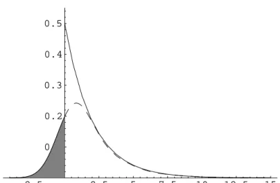
However, if the kernel function is symmetric, the estimator (1.10) will assign some weights to the undesired region where the value of x is negative [see Figure 1.2]. [This also holds for the Bhattacharyya et al. (1988) estimator.] This may cause large bias in the neighborhood of the point x= 0.

-2.5 2.5 5 7.5 10 12.5 15 0.1 0.2 0.3 0.4 0.5

Figure 1.2: Plots of density function of χ2

2 and its Jones kernel estimator with Normal

kernel. Solid line represents true density and dash line represents the estimator.

Both of the previous two density estimators have a common defect at the boundary caused by symmetric kernels. This problem is not specific to LB data. It has been recognized in density estimation for nonnegative random variables using direct data [see Silverman (1986)]. In order to overcome this defect, many methods have been proposed particularly in recent years.

Motivated by Hille’s approximation lemma [see Lemma 1.1], Chaubey and Sen (1996) proposed a smooth density estimator for nonnegative random variables.

Lemma 1.1 If u(x) is a bounded, continuous function on R+_{, then, as λ ↑ ∞,}

e−λxX

k≥0

u(k/λ)(xλ)k_/k!→u(x)

Chen (2000) obtained two density estimators with asymmetric gamma kernels instead of traditional symmetric kernels. Using gamma kernels

Kρb(x),b(t) =

tρb(x)−1_e−t/b

bρb(x)_Γ(ρb(x)), (1.11)

the density estimator proposed by Chen (2000) has the form

ˆ f(x) =n−1 n X i=1 Kρb(x),b(Xi0) (1.12) where{X0

i}ni=1 denotei.i.d. regular direct data. In his literature, Chen (2000) gave two

choices for ρb(x). One is

ρb(x) = x/b+ 1 (1.13)

which leads to density estimator ˆf1(x); the other is

ρb(x) =          x/b if x≥2b; 1 4(x/b) 2_{+ 1 if x∈[0,2b).} (1.14)

which leads to density estimator ˆf2(x). And he also showed that the MISE of ˆf2 is

lower than that of ˆf1.

Inspired by Chen’s idea and using inverse Gaussian density

KIG(m,λ)(y) = √ λ p 2πy3 exp µ − λ 2m µ y m −2 + m y ¶¶ , y >0 (1.15)

and reciprocal inverse Gaussian density

KRIG(m,λ)(z) = √ λ √ 2πz exp µ − λ 2m µ mz−2 + 1 mz ¶¶ , z >0 (1.16)

as kernels, Scaillet (2004) proposed the following two density estimators

ˆ fIG(x) =n−1 n X i=1 KIG(x,1/b)(Xi0) (1.17)

and ˆ fRIG(x) =n−1 n X i=1 KRIG(1/(x−b),1/b)(Xi0). (1.18)

Using generalized Hille’s lemma [see Lemma 1.2], Chaubey, Sen and Sen (2007) suggested a density estimator with asymmetric weights generated from gamma function, extending the estimator in Chaubey and Sen (1996).

Lemma 1.2 Let u(t) be any continuous and bounded function. Gx,n, n = 1,2, . . . is a

family of distributions with meanµn(x)and varianceh2n(x). Then we have asµn(x)→x

and hn(x)→0 ˜ u(x) = Z _∞ −∞ u(t)dGx,n(t)→u(x).

The convergence is uniform in every subinterval in which hn(x) → 0 and u(x)˜ is

uni-formly continuous.

Although Chaubey, Sen and Sen (2007) and Chen (2000) both use asymmetric gamma density function as kernels, the density estimators proposed by them are quite different in form. However, they both can be obtained by using generalized Hille’s lemma in two different ways. The density estimators proposed by Chaubey Sen and Sen (2007) are the derivatives of smooth estimators obtained by smoothing empirical function using Hille’s lemma; the density estimators in Chen (2000) and Scaillet (2004) can also be obtained by using generalized Hille’s lemma to smooth underlying density.

Besides the literature we mentioned above, there are also many other contributions made by statisticians to functional estimation for biased data. Vardi (1982) obtained the nonparametric maximum likelihood estimator for unweighted distribution function based on two sample sets, one from unweighted distribution, the other from weighted distribution. Cox’s estimator, as a NPMLE for unweighted distribution function

ob-tained only by weighted sample set, is a special case that considered by him. Vardi (1985) generalized his model to selection bias model. Wu (1996) proposed a nonpara-metric maximum likelihood smooth estimator for biased data using kernel method. Jones and Kaunamuni (1997) used fourier series method to estimate unweighted den-sity and they found that their estimator perform better than those estimators in Bhat-tacharyya et al. (1988) and Jones (1991). Lloyd and Jones (2000) proposed a nonpara-metric density estimator for biased data with unknown weight function. In their studies, the weight function is treated as a selection probability. A cross-validation method for selecting smoothing parameter in kernel density estimator with selection biased data was proposed by Wu (1997). Winter and F¨oldes (1988) derived an Kaplan-Meier type estimator for censored biased data. U˜na- ´Alarez (2002) studied its asymptotic proper-ties.

1.3

Motivation of the Estimators

The examples of biased data present themselves mostly as non-negative data where the traditional kernel methods of density estimators may not be appropriate. Recently, as mentioned previously, there have been significant advances in the area of density estimation for non-negative data. We would like to incorporate the new estimators for biased data in this thesis that is mainly motivated by the use of Hille’s lemma and Cox’s proposal for estimating the distribution function for the biased data. Chaubey and Sen (1996) proposed a smooth estimator of the distribution function for the i.i.d. case using the Hille’s lemma that incorporates Poisson weights for functional smoothing of non-negative functions. The empirical distribution function used for the i.i.d. case

may be replaced by Cox’s (1969) estimator of the distribution function for the LB data. The recent generalization [Chaubey, Sen and Sen (2007)] of Chaubey and Sen (1996), using weights generated by non-negative asymmetric kernels such as gamma kernels, may be adapted to the case of LB data as well.

1.4

Objectives

Since the LB data are commonly non-negative, the use of traditional kernel estimator may not be appropriate; it may cause large bias at the boundary. It is expected that the methods developed in Chaubey and Sen (1996) and in Chaubey, Sen and Sen (2007) can be satisfactorily adapted for the LB case and thus we have chosen to study these in the present thesis. Actually, for LB data, there are mainly two strategies to estimate unweighted density. One is, starting from Cox’s estimator, to directly estimate unweighted density [as in Jones (1991)]; the other is to estimate weighted density first and adjust it to estimate the original density [as in Bhattacharyya et al. (1988)]. Is there a relatively better strategy or do the two strategies produce similar results? We plan to find a answer to this question. In order to compare the proposed estimators, we will simulate for some standard distributions and use the mean integrated squared error (MISE) as a global measure of estimator’s behavior and mean square error (MSE) as a local indicator of estimator’s performance. Comparison between our proposed density estimators and other density estimators with asymmetric kernels will be carried out as well. Our plan includes investigating estimators of other functions, such as, distribution function estimator, hazard function estimator and mean residual life function estimator also.

1.5

Organization of the Thesis

This thesis is organized as follows. In Chapter 2, based on Cox’s estimator for dis-tribution function, we propose some disdis-tribution and density estimators with Poisson weights or asymmetric weights and study their asymptotic properties. Motivated by Chen (2000) and Scaillet (2004), we also obtain some density estimators with asym-metric kernels for LB data which are different from our proposed estimators in form. An alternative method starting from the usual empirical distribution function based on observed samples is used in Chapter 3 to find some new density and distribution function estimators with Poisson weights or asymmetric weights. Asymptotic proper-ties of these estimators are investigated as well. Through extensive simulation for some standard distributions, Chapter 4 will show how the smoothing parameters in density estimators are selected and how each density estimator performs globally and locally. We dedicate Chapter 5 to the estimators of some functionals related to density and dis-tribution functions and their asymptotic properties. These functionals include hazard function and mean residual life function. Dependency or censoring, as some situations frequently happening in statistical applications, may emerge with biased data at the same time. In future, we are planning to consider these situations as well. The details are contained in Chapter 6.

Chapter 2

Smooth Estimators of Density and

Distribution Functions Based on Cox’s

Estimator

2.1

Introduction

In this chapter, we will use Cox’s estimator (Fn) of the distribution function proposed

for the LB data to obtain some smooth estimators of the underlying true density and the corresponding distribution function. Motivated through Hille’s lemma and Cox’s proposal, it is easy to obtain smooth estimator of a distribution function in the length bias case similar to that obtained by Chaubey and Sen (1996) for thei.i.d. direct data. Since the smooth estimator is differentiable, it is reasonable to use its derivative as an estimator of the underlying density. We will consider Hille’s lemma that uses Poisson weights as well as its generalized version that uses weights generated by asymmetric ker-nels. Thus, based onFn, we get two kinds of density estimators, the first using Poisson

weights and the other using weights from asymmetric kernels. In Section 2.2, we will study theoretical properties of smooth estimators with Poisson weights, such as strong consistency and asymptotic normality. The smooth estimators include distribution and density estimator. Similar theoretical properties of estimators with asymmetric kernels are investigated in Section 2.3. In this section, a perturbation and boundary correction are applied to density estimator. They will effectively enhance the accuracy of density estimator under certain circumstances. In Chaubey et al. (2010) extensive simulation studies have been carried out to compare the density estimators using Poisson weights with kernel estimators proposed by Bhattacharyyaet al. (1988) and Jones (1991). The study in the above paper demonstrates that the kernel estimators with symmetric ker-nels do not perform very well for LB data. In order to make a fair comparison between our proposed estimators and other estimators [see Chapter 4], we only consider density estimators with asymmetric kernels in this thesis. Therefore, besides our proposed esti-mators, we will apply the idea of Chen (2000) and Scailltet (2004) also to obtain some other density estimators with asymmetric kernels in Section 2.4.

2.2

Estimators of Distribution and Density

Func-tions with Poisson Weights

2.2.1

Smooth Estimator of Cumulative Distribution Function

function, this lemma is not directly applicable, but may be considered as a motiva-tion for the suggested estimator. As we investigate the convergence properties of the proposed estimator, it becomes clear that it provides an stochastic approximation to the integral in Lemma 1.1 that replaces u(x) by F(x), which is a continuous function. The combination of Cox’s estimator and Lemma 1.1 results in the following smooth estimator of distribution function, namely,

e Fn(x) = X k≥0 pk(xλn)Fn(k/λn) (2.1) where pk(u) = u k

k!e−u and λn such that, as n → ∞, λn → ∞. Actually, λn controls the

smoothness of the smooth estimator. A stochastic choice ofλn is proposed by Chaubey

and Sen (1996, 1998) as follows.

λn =            n max{X1, . . . , Xn}

if X1 has an infinite support

n

Xn−rn+1:nlog logn

if X1 has a finite support

where rn = o(log logn), provided that E(X1) < ∞. Chaubey and Sen (2009) provide

a more comprehensive numerical study for the choice of λn in the context of density

estimation for the i.i.d. data. We use their approach for the LB data while discussing the smooth density estimation later in this section.

Similar asymptotic results as given in Chaubey and Sen (1996) for the smooth es-timator ˜Fn(x) in the non-weighted case can be established. These are given in the

following theorems. First we establish the uniform strong consistency.

Thoerem 2.1 If 0< E(X−1

1 )<∞, F(x) is continuous (a.e.) and λn→ ∞ ,then, as

n → ∞,

kFen(x)−F(x)k= sup x∈R+

Remark 2.1: In Theorem 3.1 of Chaubey and Sen (1996), additional condition onλn,

namely that n−1_λ

n→0 is assumed that is not required for the above theorem to hold.

It may be noted that the estimator in Chaubey and Sen (1996) uses truncated Poisson weights, where such a condition may be necessary.

Next, we discuss the closeness of (2.1) to the raw estimator Fn(x). This also helps

in establishing the the asymptotic distribution of the smooth estimator. Along the lines of the proof of Theorem 3.2 in Chaubey and Sen (1996) using Lemma 2.1 with bn = n−

1

2(logn)

1+θ

2 [see also the treatment in Sen (1984)], we establish the following

theorem.

Thoerem 2.2 If E(X₁−2) <∞, λn→ ∞, and n−1λn →0, f(x) is absolutely

continu-ous with bounded derivative f0_{(x) on R}+_{, then for some δ > 0, as n → ∞,}

||Fen(x)−Fn(x)||=O(n−3/4(logn)1+δ) a.s. ∀x∈R+. (2.2)

Note that √ n( ˜Fn(x)−F(x)) = √ n(Fn(x)−F(x)) + √ n( ˜Fn(x)−Fn(x))

and from Theorem 2.2, √

n( ˜Fn(x)−Fn(x)) =O(n−1/4(logn)1+δ, a.s..

Then we can see that the asymptotic law for ˜Fn(x) is same as that of Fn(x) under the

condition of Theorem 2.2. Therefore to study the asymptotic distribution of ˜Fn(x), we

just need to find out the asymptotic distribution of Fn(x). We can writeFn(x) as

Fn(x) = 1 n P_n i=1 Xi1 I{Xi ≤x} 1 n P_n i=1 Xi1 .

By the strong law of large numbers, we have 1 n n X i=1 1 Xi I{Xi ≤x}a.s.→ F(x)/µ and 1 n n X i=1 1 Xi a.s. → 1/µ. So we can expand Fn(x) as Fn(x) = F(x) +µ " 1 n n X i=1 1 Xi I{Xi ≤x} −F(x)/µ # −µF(x) " 1 n n X i=1 1 Xi − 1 µ # +O ³ (1 n n X i=1 1 Xi I{Xi ≤x} −F(x)/µ)2 +(1 n n X i=1 1 Xi I{Xi ≤x} −F(x)/µ)( 1 n n X i=1 1 Xi − 1 µ) +(1 n n X i=1 1 Xi − 1 µ) 2´ = F(x) + 1 n n X i=1 µ µ Xi I{Xi ≤x} − µF(x) Xi ¶ +O ³ (1 n n X i=1 1 Xi I{Xi ≤x} −F(x)/µ)2 +(1 n n X i=1 1 Xi I{Xi ≤x} −F(x)/µ)( 1 n n X i=1 1 Xi − 1 µ) + ( 1 n n X i=1 1 Xi − 1 µ) 2´_(a.s.).

Note that since the last term in above equation has an order op(√1_n), the asymptotic

distribution of √nFn(x) is same as that of

√ n " 1 n n X i=1 µ µ Xi I{Xi ≤x} − µF(x) Xi ¶# . (2.3)

Therefore, to obtain the asymptotic distribution ofFn(x),it is sufficient to consider the

asymptotic distribution of (2.3). For the term (2.3), we have

E Ã √ n " 1 n n X i=1 µ µ Xi I{Xi ≤x} − µF(x) Xi ¶#! = 0 and V Ã √ n " 1 n n X i=1 µ µ Xi I{Xi ≤x} − µF(x) Xi ¶#! =δ2_(x)

where δ2_{(x) =µ[}Rx 0 1tf(t)dt−2F(x) R_x 0 1tf(t)dt+ ¯µF2(x)] and ¯µ= R_∞ 0 f(t) t dt. Then we have √ n(Fn(x)−F(x))−→D N(0, δ2(x)),

Therefore we have following theorem.

Thoerem 2.3 If E(X−2

1 ) <∞, λn→ ∞, and n−1λn →0, f(x) is absolutely

continu-ous with bounded derivative f0_{(x) on R}+_{, then, as n → ∞,}

√ n(Fen(x)−F(x))−→D N(0, δ2(x)), specifically δ2(x) =µ[ Z _x 0 1 tf(t)dt−2F(x) Z _x 0 1 tf(t)dt+ ¯µF 2_(x)] where µ¯=Ef(_X1).

From Theorem 2.1 and 2.3, we see that the some of the key asymptotic properties of the raw estimators (1.3) may be exhibited also for the smooth estimator (2.1).

2.2.2

Smooth Density Estimator

SinceFen(x) converges strongly toF(x),it is reasonable to believe that their derivatives

should be close. Since we have dpk(λx)

dx =−λ[pk(λx)−pk−1(λx)],

for k ≥0,where we interpret p−1(.) = 0, the derivative of ˜Fn(x) is given by

dF˜n(x) dx =−λn " X k≥0 pk(λnx)Fn µ k λn ¶ −X k≥1 pk−1(λnx)Fn µ k λn ¶# . This simplifies to dF˜n(x) dx =λn X k≥0 pk(λnx) · Fn µ k+ 1 λn ¶ −Fn µ k λn ¶¸ .

Hence, our proposed smooth density estimator is ˜ fn(x) =λn X k≥0 pk(λnx) · Fn µ k+ 1 λn ¶ −Fn µ k λn ¶¸ . (2.4)

as the smooth estimator of density f(x). We also obtain the asymptotic properties of (2.4) as follows.

2.2.2.1 Asymptotic Properties of f˜n(x)

The strong consistency of ˜fn(.) is provided in the following theorem. Note that the

moment condition used in this theorem implies the boundedness of the density f(x).

Thoerem 2.4 If E(X−2

1 ) < ∞, f0(x) is bounded on R+ and λn = O(nα) for some

0< α <1, then, as n→ ∞,

kf˜n(x)−f(x)k−→a.s. 0

In order to obtain the weak convergence of ˜fn, we need f0(x) to satisfy a Lipschitz

order α condition. That is, for some α >0, there exits a finite positive K, such that

|f0(s)−f0(t)| ≤K|s−t|α, for everyt,s ∈R+. (2.5) If λn =O(n2/5), MSE( ˜fn(x)) achieve the lowest order [see Remark 2.2]. We establish

the following representation theorem.

Thoerem 2.5 If E(X−2

1 ) < ∞, λn = O(n2/5)(nonstochastic) and (2.5) holds, then,

for a compact set C⊂R+_,

©¡ n2/5_{[ ˜f} n(x)−f(x)]− 1 2δ2f 0_(x)¢_{, x∈C}ª _−→D _{Gaussian process}

with mean zero and covariance function γ2

xδxt where γx2 =

µ

2(πx3)−1/2f(x)δ, δxt= 0 for x6=t and 1 for x=t and δ= lim

n→∞(n

−1/5_λ1/2

Remark 2.2: In order to understand the order of bias and MSE of the density es-timator, we see that under condition (2.5) for λn = cnh using the steps in proofs of

Theorems 2.4 and 2.5, we have

Bias2( ˜fn(x))≈c−2(f0(x)/2)2n−2h (2.6) and V( ˜fn(x))≈ µ 2 r c πx3f(x)n h 2−1, (2.7) then we have MSE( ˜fn(x))≈c−2(f0(x)/2)2n−2h+ µ 2 r c πx3f(x)n h 2−1 (2.8)

When λn =cn2/5, (2.8) achieve the order O(n−4/5), which is same as classical kennel

estimators. In order to achieve the same orderO(n−4/5_{), Poisson weights estimator just}

need the information of first derivative of density. However, kennel estimators require the existence of second derivative [see Jones (1996)].

2.2.2.2 Proof of Theorems

First, we will introduce an important lemma, which plays a critical role in the proof of strong consistency of ˜fn(x).

Lemma 2.1 If E(X−2

1 )<∞ , f0(t) is bounded onR+ andbn→0, then for a sequence

{bn}n≥1 such that 0< bn−1 < O(n1−γ)(0< γ < 1),

sup t∈R+_|β|≤bnsup {|Fn(t+β)−Fn(t)−F(t+β) +F(t)|}=O(b 1 2 nn− 1 2(logn)1+θ) a.s. where θ(>0) is arbitrary.

In order to prove Lemma 2.1, we need the following two lemmas. For convenience, we denote Ui(t, β) = µ Xi I©min(t, t+β)< Xi ≤max(t, t+β) ª −|F(t+β)−F(t)| (i= 1, . . . , n) (2.9)

Lemma 2.2 If E(X₁−2)<∞, then, for any t≥0 and t+β ≥0,

1 n

n X

i=1

Ui(t, β) = o(n−1/2(logn)(1+θ)/2) a.s. (2.10)

Proof of Lemma 2.2: In order to prove the lemma, we need the Kolmogorov’s Propo-sition A in M. Lo`eve (p. 250). We state the propoPropo-sition here.

Proposition: If the integrable r.v.’s Xn are independent, then

Pσ2_(X n) a2 n < ∞ , an ↑ ∞, entails Sn−ESn an a.s. −→ 0. where Sn = P_n

i=1Xi and σ2(Xi) means the

vari-ance of Xi.

Under the assumption E(X−2

1 )<∞, for any t≥0 and t+β ≥0, we have that

∞ X n=1 σ2_(U n(t, β)) ¡ n1/2_(logn)(1+θ)/2¢2 ≤ ∞ X n=1 E(X−2 n ) ¡ n1/2_(logn)(1+θ)/2¢2 <∞.

By the Proposition of Kolmogorov , we have

P_n i=1Ui(t, β) n1/2_(logn)(1+θ)/2 a.s. −→0. (2.11) It is obvious that 1 n n X i=1 Ui(t, β) = n−1/2(logn)(1+θ)/2 P_n i=1Ui(t, β) n1/2_(logn)(1+θ)/2. (2.12)

Lemma 2.3 If E(X₁−2)<∞ and f0_{(t) is bounded on R}+_{, then there exits d >0 such}

that, for any t ≥0, 0< b−1

n < O(n1−γ)(0 < γ <1), −bn < β < bn, D=b 1 2 nn 1 2(logn)1+θ, we have P©| n X i=1 Ui(t, β)|>2dD ª ≤O(n−4_{). (2.13)}

The order O(n−4_{) does not depend on t and β.}

Proof of Lemma 2.3: First we should verify several facts. For anyδ > 2, we have

E¯¯ p X i=1 Ui(t, β) ¯ ¯δ ≤(p(logn)1+θ₎δ/2_{, (2.14)} since E¯¯ p X i=1 Ui(t, β) ¯ ¯δ =pδ_E¯_¯1 p p X i=1 Ui(t, β) ¯ ¯δ and, by Lemma 2.2, 1 p p X i=1

Ui(t, β) =o(p−1/2(logp)(1+θ)/2) a.s.

At the same time, we have

E(x1(t, β))2 = E ¡µ2 X2 1 I©min(t, t+β)< Xi ≤max(t, t+β) ª¢ −|F(t+β)−F(t)|2 = ¯¯ Z _t+β t µf(x) x dx ¯ ¯_{− |F(t+β)−F(t)|}2 _(2.15) = O(|β|). (2.16)

The conclusion of the last step follows becauseE(X−2

1 )<∞and thatf0(x) is bounded.

Since, |f(x)/x|=|f0_{(η)|< M, (η ∈(0, x) and M is finite), the first term of (2.15) has}

an order O(|β|). And since f(x) is bounded, the second term of (2.15) has an order O(β2_{) .}

So, using (2.16) and the independence of Ui(t, β)(i= 1, . . . , n), we can also establish

(2.7) in Lemma 2.1 of Babu and Singh (1978), that is

E(ξ2

1)≤O(pbn). (2.17)

Substituting (2.4) in Lemma 2.1 of Babu and Singh (1978) with (2.14), takingδ = 60/γ and p= [nγ/2_{], and following the proof of Lemma 2.1 of Babu and Singh (1978), we can}

obtain the result.

Remark 2.3: The second term exp(−8D2_n−1_b−1

n ) in (2.1) of Babu and Singh(1978)

disappears in our inequality, because under our choice of D, this term is much smaller than O(n−4_).

Proof of Lemma 2.1 : Let

Hn(t, β) =Fn(t+β)−Fn(t)−F(t+β) +F(t).

Since Fn(t+β)−Fn(t) can be expanded as

Fn(t+β)−Fn(t) = 1 n n X i=1 µ Xi I{t < Xi ≤t+β} −[F(t+β)−F(t)]¡1 n n X i=1 µ Xi −1¢ +o¡[F(t+β)−F(t)]¡1 n n X i=1 µ Xi −1¢¢ a.s., (2.18) we have |Hn(t, β)| ≤Jn1(t, β) +Jn2(t, β) +o(Jn2(t, β)) a.s. (2.19) where Jn1(t, β) = 1 n ¯ ¯Xn i=1 Ui(t, β) ¯ ¯ _(2.20)

and Jn2(t, β) = ¯ ¯_{[F(t+β)−F(t)]}¡1 n n X i=1 µ Xi −1¢¯¯. (2.21) For (2.20), first we consider that t is fixed. Using Lemma 2.3, following the proof of Lemma 1 of Bahadur (1966), we can claim that

sup |β|≤bn {|Jn1(t, β)|}=O(b 1 2 nn− 1 2(logn)1+θ) a.s.

Furthermore, sinceO(b12 nn−

1

2(logn)1+θ) does not depend ontandf0(t) is bounded, using

the same technique as in Sen and Ghosh (1971), we can extend the result for t to the whole real line, that is

sup t∈R+ sup |β|≤bn {|Jn1(t, β)|}=O(b 1 2 nn− 1 2(logn)1+θ) a.s. (2.22)

At the same time, in Lemma 2.2, let t= 0 andβ →+∞, then we have

¡1 n n X i=1 µ Xi

−1¢=o(n−1/2(logn)(1+θ)/2) a.s. (2.23) Since f(t) is bounded(because E(X−2

1 )<∞) as well, we have sup t∈R+ sup |β|≤bn ¯ ¯_{F(t+β)−F(t)}¯¯_{=O(bn). (2.24)}

For (2.21), by (2.23) and (2.24), we have

sup t∈R+ sup |β|≤bn {|Jn2(t, β)|}=o(bnn− 1 2(logn)(1+θ)/2) a.s. (2.25)

By (2.19), (2.22) and (2.25), we can establish the Lemma 2.1.

After all of these preparations, we can prove the Theorem 2.4.

Proof of Theorem 2.4: By the proof of Theorem 4.1 of Chaubey and Sen (1996), we just need to show that, when t belongs to some finite interval [0,C], we have (2.4),

since we can deliberately choose C such that when t belongs to interval (C,+∞), ˜fn(t)

and f(t) can both be made sufficiently small. We can write ˜ fn(x) = λn ©X k≥0 pk(xλn)[F( k+ 1 λn )−F( k λn )] +X k≥0 pk(xλn)[Fn( k+ 1 λn )−Fn( k λn )−F(k+ 1 λn ) +F( k λn )]ª = Tn1(x) +Tn2(x). (2.26)

Using Lemma (2.1) by taking bn = 1/λn, we have

sup k≥0{|Fn( k+ 1 λn )−Fn( k λn ) − F(k+ 1 λn ) +F( k λn )|} = O(λ−1/2 n n−1/2(logn)1+θ) a.s. (2.27)

By (2.27) and the fact that P

k≥0

pk(xλn) = 1, we have

sup

x∈R+

{|Tn2(x)|}=O(λ1n/2n−1/2(logn)1+θ) a.s. (2.28)

which tends to 0 almost surely as n → ∞provided that λn=O(nα)(0< α <1).

At the same time, according to the proof of Theorem 4.1 of Chaubey and Sen (1996), under the assumption of boundedness of f0_{(x), we have}

sup

t∈[0,C]

{|Tn1(x)−f(x)|} →0 a.s. (2.29)

By (2.28) and (2.29), we obtain the theorem. The proof is complete.

Proof of Theorem 2.5: By (2.5), we have

˜

fn(x) = f(x) +

1 2λn

Using Taylor’s expansion which is similar to (2.18), we can write Tn2(x) = λn X k≥0 pk(xλn) ©¡1 n n X i=1 µ Xi I{ k λn < Xi ≤ k+ 1 λn } −[F(k+ 1 λn )−F( k λn )]¢ª −λn X k≥0 pk(xλn) © [F(k+ 1 λn )−F( k λn )]¡1 n n X i=1 µ Xi −1¢ª+o(1 n n X i=1 µ Xi −1) = Tn3(x)−Tn4(x) +o(1 n n X i=1 µ Xi −1) a.s. (2.31)

For the leading term Tn3(x), following the proof of Theorem 4.2 of Chaubey and Sen

(1996), we can show that

V(Tn3(x))≈ µ 2(πx 3₎−1/2_f(x)(λ1/2 n /n) (2.32) and, for s6=t, as n→ ∞, Cov[Tn3(s), Tn3(t)] =O( 1 n). (2.33) Moreover, sinceTn4(x) =O( 1 n P_n i=1 µ Xi

−1) =o(n−1/2_(logn)(1+θ)/2_{), the order ofT}

n2(x)

is determined by the order of Tn3(x).

From (2.30), we can see that the asymptotic normality ofTn2(x) leads to the

asymp-totic normality of ˜fn(x). by proper choice of λn. By (2.30), (2.31), (2.32) and (2.33),

following the proof of Theorems 4.1 and 4.2 of Chaubey and Sen (1996), we can complete the proof of the theorem.

2.3

Estimators of Distribution and Density

Func-tions with Asymmetric Kernels

2.3.1

Smooth Estimator of Distribution Function with

Asym-metric Kernels

As in Chaubey, Sen and Sen (2007), let Qvn(x) be a family of distributions on [0,∞)

with mean 1 and variancev2

nwherevn→0 asn → ∞. SubstitutingFn(t) andQvn(t/x)

for u(t) andGx,v(t) in Lemma 1.2 respectively, we have the following smooth estimator

of F(x): e F+ n(x) = Z _∞ 0 Fn(t)dQvn(t/x). (2.34)

An alternative formula of (2.34) is given by

e F+ n(x) = 1− P_n i=1_PXi1 Qvn(Xix ) n i=1 Xi1 , (2.35)

where Qvn is a family of distributions as described earlier.

2.3.1.1 Asymptotic Properties

By the uniform strong convergence of (1.3)

sup

x≥0

|Fn(x)−F(x)|−→a.s. 0

and the form of Fe+

n(x) (2.34), it is easy to obtain the uniform strong convergence of e

F+

n(x) as follows.

Thoerem 2.6 If 0< E(X−1

1 )<∞ and F(x) is continuous (a.e.), then, as vn →0,

kFe+ n(x)−F(x)k= sup x∈R+ {|Fe+ n (x)−F(x)|} a.s. −→0

The asymptotic normality of Fe+

n(x) is given by the following theorem.

Thoerem 2.7 IfE(X−2

1 )<∞,

√ nv2

n→0, f(x)is absolutely continuous with bounded

derivative f0_{(x) on R}+_{, then, as n→ ∞,} √ n(Fe_n+(x)−F(x))−→D N(0, δ2(x)) where δ2_{(x) =µ[} Z _x 0 1 tf(t)dt−2F(x) Z _x 0 1 tf(t)dt+ ¯µF 2_(x)] where µ¯=Ef(_X1₁).

Proof: First, by (2.35), we write

e F+ n(x) = 1 n P_n i=1 Xi1 [1−Qvn(Xix )] 1 n P_n i=1Xi1 , (2.36)

then we can expand Fe+

n(x) as e F+ n(x) ≈ F(x) + ¡µ n n X i=1 1 Xi [1−Qvn( Xi x )]−F(x) ¢ −µF(x)¡1 n n X i=1 1 Xi − 1 µ ¢ = F(x) + 1 n n X i=1 µ Xi [1−Qvn( Xi x )−F(x)]. (2.37) Let ξi = µ Xi [1−Qvn( Xi x )−F(x)]. (2.38)

In order to obtain the theorem, it is sufficient to show that, as vn → 0, E(

√

nξ1)→ 0

E(ξ1) = Z _∞ 0 µ t[1−Qvn( t x)−F(x)]g(t)dt = Z _∞ 0 [1−Qvn( t x)]f(t)dt−F(x) = Z _∞ 0 F(t)qvn(t x) dt x −F(x) = Z _∞ 0 F(xy)qvn(y)dy−F(x). (2.39)

Using the Taylor’s expansion of F(xy) at the point y = 1

F(xy) =F(x) +xf(x)(y−1) + x2f0(ηx)

2 (y−1)

2 _(2.40)

where η is between 1 and y, and the fact thatf0_{(x) is bounded, we can show that}

E(ξ1) =O(v2n). (2.41)

This means that E(√nξ1)→0.

On the other hand, we have

E(ξ2 1) = E ¡ µ X1 [1−Qvn( X1 x )−F(x)] ¢₂ = E¡µ2 X2 1 [1−Qvn( Xi x ] 2¢ −2F(x)E¡µ2 X2 1 [1−Qvn( Xi x ] ¢ +F2_(x)E¡µ2 X2 1 ¢ (2.42) Furthermore, we have E¡µ 2 X2 1 [1−Qvn(Xi x )] 2¢ _{= µ} Z _∞ 0 f(t) t [1−Qvn(t/x)] 2_dt = 2µ Z _∞ 0 H(t)[1−Qvn(t/x)]qvn(t/x) dt x = 2µ Z _∞ 0

where H(x) = R₀xf(_tt)dt. Using the Taylor’s expansion of H(xy) with respect to y at the point y0 = 1 H(xy) = H(x) +xf(ηx) ηx (y−1) = H(x) +xf(ηx)−f(0) ηx (y−1) = H(x) +xf0_{(τ)(y−1) (2.44)}

where η is between 1 and y and τ ∈(0, xη). In the step above, we use a fact f(0) = 0, because E( 1 X2 1)<∞. Sincef 0_{(x) is bounded, we have} E¡µ 2 X2 1 [1−Qvn(Xi x )] 2¢ _{= µH(x)} +O( Z _∞ 0

[1−Qvn(y)]qvn(y)(y−1)dy). (2.45)

Note that

O(|

Z _∞

0

[1−Qvn(y)]qvn(y)(y−1)dy|) ≤ O(2

Z _∞ 0 qvn(y)|y−1|dy) ≤ O(2[ Z _∞ 0 qvn(y)(y−1)2dy)]1/2) = O(vn), (2.46) so, we have, as vn→0, E¡µ2 X2 1 [1−Qvn( Xi x )] 2¢ _{→µH(x). (2.47)} Similarly, we have 2F(x)E¡µ2 X2 1 [1−Qvn( Xi x ] ¢ = 2µF(x) Z _∞ 0 H(xy)qvn(y)dy = 2µF(x)H(x) +O( Z _∞ 0 qvn(y)|y−1|dy) → 2µF(x)H(x). (2.48) By (2.42), (2.47) and (2.48), we have E(ξ2 1)→µ[H(x)−2F(x)H(x) + ¯µF2(x)]. (2.49)

The proof is complete.

2.3.1.2 MSE

According to the proof of Theorem 2.3, we have

Bias(Fe+ n(x)) = x2 2 f 0_(x)v2 n+o(v2n) (2.50) and V(Fe+ n(x)) = µ n[ Z _x 0 1 tf(t)dt−2F(x) Z _x 0 1 tf(t)dt+ ¯µF 2_{(x)] +o(}1 n). (2.51) So MSE(Fe_n+(x)) = µ n[ Z _x 0 1 tf(t)dt−2F(x) Z _x 0 1 tf(t)dt+ ¯µF 2_(x)] +x4 2 f 0₂ (x)v4 n+o( 1 n +v 4 n) (2.52)

2.3.2

Density Estimator using Asymmetric Kernels

˜ fn(x) = 1 x2 P_n i=1qvn(Xix ) P_n i=1 Xi1 (2.53)

as a smooth estimator of f(x) whereqvn(t) = _dtdQvn(t).

However, (2.53) may not be defined at x = 0, except in cases where limx→0f˜n(x)

exists. Moreover, this limit is zero, which is acceptable only we are estimating f(x) with f(0) = 0. This situation also occurs in estimating density with direct data [see Chaubey, Sen and Sen (2007)]. In their paper, they considered a perturbed version of the density estimator, replacing Qvn(./x) by Qvn(./(x+²)), ²n ↓ 0 as n → ∞. This is

variance is (x+²n)2vn2 →0.Motivated by their idea, the perturbed version of (2.53) is given by ˜ f+ n(x) = 1 (x+εn)2 P_n i=1qvn(x+Xiεn) P_n i=1 Xi1 . (2.54) 2.3.2.1 Asymptotic property of f˜+ n(x) Thoerem 2.8 If

A. f(·) is Lipschitz continuous on [0,∞) and E(X−1

1 )<∞;

B. sup_x≥0R₀∞| d

dx[x+1εnqvn(x+tεn)]|dt=o((

log logn n1/2 )−1); C. sup_u>0,v>0uqv(u)<∞;

D. vn→0, εn→0 as n→ ∞; then we have sup x≥0 |f˜+ n(x)−f(x)| a.s. −→0 as n→ ∞.

Proof: We can write

˜ f_n+(x) = d dx Z Fn(t)[ 1 x+εn qvn( t x+εn )]dt = Z Fn(t) d dx[ 1 x+εn qvn( t x+εn )]dt (2.55)

Using the uniform strong convergence of Fn(x)

sup

x≥0|Fn(x)−F(x)|

a.s.

−→0. (2.56)

and following the proof of Theorem 3 of Chaubey, Sen and Sen (2007), we can obtain the theorem.

Thoerem 2.9 If