CLINICAL SCIENCES, INTERVENTION AND TECHNOLOGY
Division for Medical Imaging, Function and Technology
Karolinska Institutet, Stockholm, Sweden
A TINY GLIMPSE INTO THE HUMAN
BRAIN USING MODEL-FREE ANALYSIS
FOR RESTING-STATE FMRI DATA
Yanlu Wang
Stockholm 2015
CLINICAL SCIENCES, INTERVENTION AND TECHNOLOGY
Division for Medical Imaging, Function and Technology
Karolinska Institutet, Stockholm, Sweden
A TINY GLIMPSE INTO THE HUMAN
BRAIN USING MODEL-FREE ANALYSIS
FOR RESTING-STATE FMRI DATA
Yanlu Wang
All previously published papers were reproduced with permission from the publisher. Published by Karolinska Institutet.
Printed by E-Print AB 2015 © Yanlu Wang, 2015 ISBN 978-91-7676-109-0
All previously published papers were reproduced with permission from the publisher. Published by Karolinska Institutet.
Printed by E-Print AB 2015 © Yanlu Wang, 2015 ISBN 978-91-7676-109-0
MODEL-FREE ANALYSIS FOR RESTING-STATE FMRI
DATA
THESIS FOR DOCTORAL DEGREE (Ph.D.)
ByYanlu Wang
Principal Supervisor: Prof. Tie-Qiang Li Karolinska Institute
Department of Clinical Sciences, Intervention and Technology
Division for Medical Imaging, Function and Technology
Co-supervisor(s): Prof. Mussie Msghina Karolinska Institutet
Department of Clinical Neuroscience
Opponent:
Prof. Peter Lundberg Linköping University
Department of Medical and Health Sciences Division of Radiological Sciences
Examination Board: Prof. Pia Sundgren Lund University
Department of Clinical Sciences, Lund Division for Diagnostic Radiology Prof. Svein Kleiven
Royal Institute of Technology (KTH) School of Technology and Health Department of Medical Engineering Unit of Neuronics
Prof. Istvan Furo
Royal Institute of Technology (KTH) School of Chemical Science and Engineering Department of Chemistry
Division for Applied Physical Chemistry
MODEL-FREE ANALYSIS FOR RESTING-STATE FMRI
DATA
THESIS FOR DOCTORAL DEGREE (Ph.D.)
ByYanlu Wang
Principal Supervisor: Prof. Tie-Qiang Li Karolinska Institute
Department of Clinical Sciences, Intervention and Technology
Division for Medical Imaging, Function and Technology
Co-supervisor(s): Prof. Mussie Msghina Karolinska Institutet
Department of Clinical Neuroscience
Opponent:
Prof. Peter Lundberg Linköping University
Department of Medical and Health Sciences Division of Radiological Sciences
Examination Board: Prof. Pia Sundgren Lund University
Department of Clinical Sciences, Lund Division for Diagnostic Radiology Prof. Svein Kleiven
Royal Institute of Technology (KTH) School of Technology and Health Department of Medical Engineering Unit of Neuronics
Prof. Istvan Furo
Royal Institute of Technology (KTH) School of Chemical Science and Engineering Department of Chemistry
To my dearly beloved wife, whom gives purpose to my resting-state functional connectivity networks.
To my dearly beloved wife, whom gives purpose to my resting-state functional connectivity networks.
ABSTRACT
Resting-state functional Magnetic Resonance Imaging (fMRI) acquires four dimensional data that indirectly depicts human brain activity. Within these four dimensional datasets reside resting-state functional connectivity networks (RFNs), depicting how the human brain is organized functionally. This series of studies delve into the use of data-driven analysis methods for resting-state fMRI data. Their strengths were explored and their weaknesses tackled, both in their methodologies and applications, all in hope to gain a better understanding of the data, and thereby how the brain function.
The journey begins through the usage of one of the most common data-driven analysis methods in use today: Independent Component Analysis (ICA). ICA requires no user input parameter apart from the input dataset and the number of output Independent Components (NIC). The requirement of the NIC, a priori, is troubling as the inherent number of Independent Components (ICs) that exists within non-simulated datasets is unknown, due to the existence of various noise and artefact sources to differing degrees. Furthermore, comparing datasets using ICA is problematic because of the inherently different dimensionality of different datasets. To investigate the effects of NIC on the ICA output results, a classification framework based on Support Vector Machines (SVM) was implemented to automatically classify ICs as either potential RFNs, or noise/artefact signal. This feature-optimized classification of ICs with SVM, or FOCIS, framework uses features derived from verbal instructions for manual visual inspection of ICs. With only few significant features selected through iterative feature-selection and a small training set, the classification framework performed well with over 98% in overall accuracy for group ICA output results. Analysis of different resting-state fMRI datasets using FOCIS indicated that the specification of NIC can critically affect the ICA results on resting-state fMRI data. These changes are complex and are individually different from one another, irrespective whether the IC is a potential RFN or artefact/noise signals. Applying this knowledge on group comparison studies, ICA was used to study migraine patients undergo kinetic oscillation stimulation treatment. The immediate effects of the treatment allows direct correlation of a patient’s pain levels with changes in their RFNs. Differences in RFNs that include areas in the midbrain and limbic system regulating the central nervous system were discovered in migraine patients compared to healthy control group. Overlapping areas were also shown to be affected by the treatment. These results provide supporting evidence for the hypothesis that the treatment affects and regulates the parasympathetic autonomic reflex, alleviating migraine symptoms.
Hierarchical clustering is another data-driven analysis method that is almost devoid of all user-input parameters. The algorithm naturally stratifies data into a hierarchical structure. It is believed that brain function is hierarchically organized, so an algorithm which reflects this aspect is a seemingly excellent choice to use for analyzing the resting-state fMRI data. A hierarchical clustering analysis framework was developed to extract RFNs from resting-state fMRI data with full brain coverage at voxel level. The RFNs identified using hierarchical clustering conforms to those identified previously using other data processing techniques, such
hierarchical tree (dendrogram). This was fully utilized though extensions in the framework for cluster evaluation. Extending the hierarchical clustering framework with the cluster evaluation pipeline allowed extraction of functional subdivisions of known RFNs. This demonstrated that not only can hierarchical clustering be used to extract the modular organization at the scale of large systems for entire RFNs, but can also be used to derive the functional subdivision of RFNs and provide a consistent method of analysis at different levels of detail. The sub-networks extracted using hierarchical clustering reveals the intrinsic functional connectivity amongst the subnetworks within RFNs and provide clues for further exploring the potential for currently unknown functional junctions within RFNs.
hierarchical tree (dendrogram). This was fully utilized though extensions in the framework for cluster evaluation. Extending the hierarchical clustering framework with the cluster evaluation pipeline allowed extraction of functional subdivisions of known RFNs. This demonstrated that not only can hierarchical clustering be used to extract the modular organization at the scale of large systems for entire RFNs, but can also be used to derive the functional subdivision of RFNs and provide a consistent method of analysis at different levels of detail. The sub-networks extracted using hierarchical clustering reveals the intrinsic functional connectivity amongst the subnetworks within RFNs and provide clues for further exploring the potential for currently unknown functional junctions within RFNs.
LIST OF SCIENTIFIC PAPERS
I. Analysis of Whole-Brain Resting-State fMRI Data Using Hierarchical
Clustering Approach, Wang Y.; Li TQ., PLoS ONE, 2013, 8 (10)
II. Dimensionality of ICA in resting-state fMRI investigated by featurre
optimized classification of independent components with SVM, Wang Y.; Li TQ.; Frontiers in Human Neuroscience, 2015, 9 (259)
III. Studying Sub-dendrograms of Resting-state Functional Networks with
Voxel-wise Hierarchical Clustering, Wang Y.; Msghina M.; Li TQ., Frontiers in Human Neuroscience, submitted 2015, 8
IV. Resting-state fMRI Study of Acute Migraine Treatment with Kinetic
Oscillation Stimulation in Nasal Cavity, Li TQ.; Wang Y.; Juto JE., manuscript
1 Introduction ... 8
1.1 What is resting-state fMRI ... 8
1.2 Analysis methods... 9
2 Independent Component Analysis ... 12
2.1 Interpreting blind-source separation ... 13
2.2 Dimensionality of resting-state fMRI datasets ... 13
2.3 Application on group comparison studies ... 14
2.4 Treating migraine with kinetic oscillation Stimulation ... 14
2.5 Study outline ... 15
2.6 FOCIS... 16
2.7 ICA analysis ... 16
2.8 Classification and dimensionality investigation ... 17
2.9 Kinetic Oscillation Stimulation treatment effects on migraine patients ... 19
3 Hierarchical Clustering ... 22
3.1 How Hierarchical Clustering Works ... 22
3.2 On Distance Measures ... 23
3.3 On Linkage... 24
3.4 Data mining and visualization ... 24
3.5 Definition of RFNS and sub-networks ... 26
3.6 cluster Evaluation and Where to stop cutting ... 27
3.7 Study Outline ... 28
3.8 Implementing the hierarchical clustering framework ... 28
3.8.1 The necessity of optimizations ... 28
3.8.2 Memory allocation ... 29
3.8.3 Parallel Programming ... 29
3.8.4 Dimensionality reduction ... 29
3.8.5 Libraries ... 29
3.9 Hierarchical clustering and ICA results ... 30
3.10 Functional hierarchies ... 30 4 Summary ... 34 5 Future Perspectives ... 35 6 Acknowledgements ... 37 References ... 39 1 Introduction ... 8
1.1 What is resting-state fMRI ... 8
1.2 Analysis methods... 9
2 Independent Component Analysis ... 12
2.1 Interpreting blind-source separation ... 13
2.2 Dimensionality of resting-state fMRI datasets ... 13
2.3 Application on group comparison studies ... 14
2.4 Treating migraine with kinetic oscillation Stimulation ... 14
2.5 Study outline ... 15
2.6 FOCIS... 16
2.7 ICA analysis ... 16
2.8 Classification and dimensionality investigation ... 17
2.9 Kinetic Oscillation Stimulation treatment effects on migraine patients ... 19
3 Hierarchical Clustering ... 22
3.1 How Hierarchical Clustering Works ... 22
3.2 On Distance Measures ... 23
3.3 On Linkage... 24
3.4 Data mining and visualization ... 24
3.5 Definition of RFNS and sub-networks ... 26
3.6 cluster Evaluation and Where to stop cutting ... 27
3.7 Study Outline ... 28
3.8 Implementing the hierarchical clustering framework ... 28
3.8.1 The necessity of optimizations ... 28
3.8.2 Memory allocation ... 29
3.8.3 Parallel Programming ... 29
3.8.4 Dimensionality reduction ... 29
3.8.5 Libraries ... 29
3.9 Hierarchical clustering and ICA results ... 30
3.10 Functional hierarchies ... 30
4 Summary ... 34
5 Future Perspectives ... 35
6 Acknowledgements ... 37
LIST OF ABBREVIATIONS
(IN ORDER OF APPEARANCE)(f)MRI (functional) Magnetic Resonance Imaging
BOLD Blood Oxygen Level Dependent (contrast)
RFN Resting-state Functional connectivity Network
GLM General Linear Model
ROI Region Of Interest
ICA Independent Component Analysis
IC Independent Component
NIC Number of Independent Components (parameter)
KOS Kinetic Oscillation Stimulation (treatment)
SVM Support Vector Machines
FOCIS Feature Optimized Classification of Independent components using
Support vector machines (framework)
ANOVA ANalysis Of VAriance
CC (cross-) Correlation Coefficient
LIST OF ABBREVIATIONS
(IN ORDER OF APPEARANCE)(f)MRI (functional) Magnetic Resonance Imaging
BOLD Blood Oxygen Level Dependent (contrast)
RFN Resting-state Functional connectivity Network
GLM General Linear Model
ROI Region Of Interest
ICA Independent Component Analysis
IC Independent Component
NIC Number of Independent Components (parameter)
KOS Kinetic Oscillation Stimulation (treatment)
SVM Support Vector Machines
FOCIS Feature Optimized Classification of Independent components using
Support vector machines (framework)
ANOVA ANalysis Of VAriance
PREFACE
In the digital age, large amounts of data seems to be easily acquired. A system can be set up with relative ease to acquire enormous amounts of data. The difficult part remains to extract meaningful information from a seemingly overwhelming amount of gathered data. One then, can one interpret the data, and draw useful conclusions from within. Functional magnetic resonance imaging produces large quantities of data of the human brain; and within, hides the patterns depicting shadows of our consciousness. To better understand the human brain and ourselves, tools were created to extract meaningful information from data that are difficult immediately grasp with our minds.
As tradition dictates, the following sections will include a summary of the articles I have published (and yet to publish) throughout my studies. This is often done in a standard, de-facto format, for scientific articles today. Yet, this format does not lend itself for the purpose tying in different studies into a coherent whole, with a consistent pattern of thought. This is why I have attempted to, as much as possible, write this summary in prose, believing that this format will better reflect my thought processes throughout my studies. Those of you readers with an undying need to see scientific rigor in their predefined sections, the published articles (and manuscripts) can be found appended as usual. But for those who do not feel the urge to see sections called “Materials and Methods” and “Conclusion” in everything they read, you’re welcome (or at least I tried).
Aug 2015
PREFACE
In the digital age, large amounts of data seems to be easily acquired. A system can be set up with relative ease to acquire enormous amounts of data. The difficult part remains to extract meaningful information from a seemingly overwhelming amount of gathered data. One then, can one interpret the data, and draw useful conclusions from within. Functional magnetic resonance imaging produces large quantities of data of the human brain; and within, hides the patterns depicting shadows of our consciousness. To better understand the human brain and ourselves, tools were created to extract meaningful information from data that are difficult immediately grasp with our minds.
As tradition dictates, the following sections will include a summary of the articles I have published (and yet to publish) throughout my studies. This is often done in a standard, de-facto format, for scientific articles today. Yet, this format does not lend itself for the purpose tying in different studies into a coherent whole, with a consistent pattern of thought. This is why I have attempted to, as much as possible, write this summary in prose, believing that this format will better reflect my thought processes throughout my studies. Those of you readers with an undying need to see scientific rigor in their predefined sections, the published articles (and manuscripts) can be found appended as usual. But for those who do not feel the urge to see sections called “Materials and Methods” and “Conclusion” in everything they read, you’re welcome (or at least I tried).
1 INTRODUCTION
The following sections provide background information for those not directly involved in the field of functional Magnetic Resonance Imaging (fMRI) to comprehend and appreciate the thought patterns throughout my studies. This section could, and should, be averted by those with an established understanding of resting-state fMRI and its processing methods.
1.1 WHAT IS RESTING-STATE FMRI
Magnetic Resonance Imaging (MRI) is a medical imaging technique that uses the differing quantum mechanical properties of different types of tissue to form an image noninvasively. MRI is completely noninvasive, unlike most other medical imaging techniques such as X-ray, Computed Tomography, and Positron Emission Tomography, all of which requires one to be subjected to ionizing radiation to form a meaningful image.
In neuroimaging, MRI scans are traditionally used to visualize the anatomical structure of the brain. fMRI is a special type of brain scanning technique, using MRI that visualizes the brain’s function by using a technique called Blood Oxygen Level Dependent (BOLD) contrast [1]. The theory behind BOLD contrast is as follows: When neurons in the brain activate during task, they will absorb energy in the form of oxygen and other nutrients from the surrounding capillaries. This causes a slight drop in blood oxygen levels in the capillaries surrounding areas of brain activity. The body will sense this drop and over-compensate by flushing fresh, oxygenated, blood to that area in excess [2, 3]. This phenomenon is called the hemodynamic response, and is important due to two reasons: (1) It can be modelled through the hemodynamic response function and (2) It can be measured using MRI because oxygenated blood and deoxygenated blood have different magnetic properties [4].
The purpose of task based fMRI (or paradigm fMRI) is to visualize regions of the brain responsible for processing specific external stimuli. In a task based fMRI experiment, a subject is scanned continuously for a duration about 6-12 minutes using a special type of pulse-sequence. This sequence (typically based on an echo-planar imaging technique [5]), is strongly T2*-weighted and sensitive to BOLD contrast. The sequence is also very fast such that an image of an entire brain is acquired in the duration of between 0.5 to 3.0 seconds. It continuously scans the brain much like sequential shooting options for digital cameras. During the scan, the subject is exposed to predefined stimuli, designed to activate specific regions of the brain at timed intervals. The stimulus can be as simple as a sound or picture, to more complex tasks such as emotional or social thought processing tasks. After processing, the specific regions of the brain responsible for processing the presented stimuli can be visualized in vibrant colors as overlays on top of a structural image of the brain.
Resting-state fMRI is simply task-based fMRI without a task. In a resting-state fMRI experiment, the subject is scanned in the same fashion as task-based fMRI, but without any stimulus presented during scanning. The data acquired in this fashion would reflect thought patterns associated with the wandering mind (unless the subject falls asleep). In one respect,
the name resting-state fMRI is misleading as the brain is never truly at rest. One is typically instructed to not think about anything in particular, instead letting thoughts flow at will. Different regions of the brain work in synchronous with each other, for any particular thought. The regions of the brain working in synchrony for any particular thought, is known as (resting-state) functional connectivity networks, or RFNs. Even without a particular cue or stimulus, the mind wanders during the scan, and this mind wandering results in different thoughts which activates different RFNs. Multiple RFNs are consistently identified, many corresponding to task activated areas from task based fMRI studies [6, 7] (some are uniquely identified in resting-state fMRI, such as the default-mode network [8, 9]). Instead of just extracting one RFN from each scanning session, one hopes to extract multiple (if not “all”) RFNs residing within resting-state fMRI data, “all at once”.
1.2 ANALYSIS METHODS
fMRI data as obtained from the MRI scanner does not look anything similar to the vibrant images in the “Results” section of a published scientific paper. Many stages of processing and analysis is required to produce the final image. It should be noted that, before the actual analysis is performed, the acquired fMRI data should be subjected to multiple computational steps, collectively known as the preprocessing pipeline. The preprocessing steps are purposed to remove confounding factors in the fMRI data. Since preprocessing is not the main focus, further explanation shall be abstained due to space constraints. Pre-processing is an essential and important step in the analysis, and at times, more complex and heavily scrutinized than the analysis method and is a subject on its own. There are many excellent review articles explaining the most common pre-processing steps in more details [10].
Figure 1: Illustrative overview of GLM-based analysis methods for task-based fMRI
For task-based fMRI, the conventionally used analysis method is to process each voxel (volumetric pixel) individually using the General Linear Model (GLM). This method is commonly known as the GLM-method [11, 12]. It is comparatively simple and easily comprehensible. The stimulus onset timing and duration forms basis of the model. It is then convolved with the hemodynamic response function, to create an “ideal” time-course for the
particular stimulus. The ideal course is then used to assess each voxel of the brain’s course using the general linear model. Voxels with courses similar to the “ideal” time-course will have a high t-score and those who do not will have a low t-score. After this statistical mapping, the t-scores for all voxels are thresholded to obtain only the significant voxels. The thresholded t-map is then color mapped with bright colors and presented on top a structural image of the brain. This entire workflow can be seen illustrated in Figure 1. GLM-based statistical parametric mapping technique is conceptually transparent and relatively easy to perform, especially with ready-made software now readily available.
Figure 2: Task based fMRI analysis relies on the explicit timing of the stimulus presented during the scan. Without the presence of a task and its timing information in resting-state fMRI, the analysis method becomes much less intuitive
The unfortunate problem with the GLM-method is that it does not readily translate to being applied to resting-state fMRI data (Figure 2). Conventionally, the seed-voxel analysis method [13] was used on resting-state fMRI data. This method is actually a translation of the GLM-method as follows: One would draw a Region of Interest (ROI), extract the average time-course from all voxels inside the ROI, and use the averaged time-course as the “ideal” time-course to access all other voxels using GLM. This works relatively well and to this day is still frequently used, however; one fundamental problem still persists: In task based fMRI, one’s interests are mostly predefined by the stimuli chosen at the time of data acquisition. For example, if an fMRI experiment is performed using an auditory stimulus, it would be the auditory network that is of interest and not the visual network. The intention of resting-state fMRI is to extract as many RFNs simultaneously without knowing what lies within the data prior to analysis. To this end, the seed-voxel analysis method is just simply lacking. Furthermore, the ROI dictates the outcome of the analysis. The ROIs are typically drawn by the hands of the individual user, which will vary from one individual to the next.
Researchers needed model-free analysis methods that do not require prior hypothesis or ROIs to be drawn beforehand to fully explore resting-state fMRI data. A consequence of this is that the model-free analysis methods do not often even require a solid hypothesis to be formulated prior to analysis. Hence, they are not as transparent and comprehensible due to their complexity and generality. Interpreting the results can be difficult as a drawback of their ability to function, without a solid hypothesis, is that their output may be vague in meaning.
Researchers needed model-free analysis methods that do not require prior hypothesis or ROIs to be drawn beforehand to fully explore resting-state fMRI data. A consequence of this is that the model-free analysis methods do not often even require a solid hypothesis to be formulated prior to analysis. Hence, they are not as transparent and comprehensible due to their complexity and generality. Interpreting the results can be difficult as a drawback of their ability to function, without a solid hypothesis, is that their output may be vague in meaning.
2 INDEPENDENT COMPONENT ANALYSIS
ICA is a popular and widely used data-driven method to analyze resting-state fMRI data [14]. How ICA works may not be very intuitive for most, but with software packages like FSL [15] (http://fsl.fmrib.ox.ac.uk/fsl/) and GIFT (http://www.nitrc.org/projects/gift) almost anyone can use ICA to analyze resting-state fMRI data.
This would normally be the place to get into the technical details of ICA, but it shall be omitted here. For those interested in the technical details behind ICA, certainly one can easily find better source of information than what can be managed on these pages. For introductory purposes, knowing how ICA functions conceptually will suffice. What is relevant, is how to interpret the output results from ICA analysis, and how to correctly apply ICA analysis on group comparison studies.
How ICA works conceptually can be intuitively explained through noise cancellation on modern mobile phones: There are usually many noise sources during a mobile phone conversation in cities. Speaking on your phone in a crowded café by a busy street is not a big problem for the modern mobile phone. Inside your phone lies a chip running a variant of ICA which decomposes the sound signal received through the microphone to its individual sources, including your voice, other people’s conversations, and the traffic noise outside for example. Once the sound sources have been isolated, all noise sources can be eliminated to transmit only the sound of your voice to the recipient. How the algorithm identifies your voice amongst the noise signals is another (more difficult) question altogether. The entire process is illustrated in Figure 3.
Figure 3: Illustrative example of how ICA can be used to separate signal sources from a mixture of sounds to filter out unwanted noise sources during a typical mobile phone conversation.
In the case of ICA applied to resting-state fMRI data, ICA takes the entire 4D dataset as an input and outputs a predefined number of independent components (ICs), with each component representing a potential signal source, that altogether form the original input data [16]. Each IC (time-course) is then mapped spatially using statistical mapping to form activation maps corresponding to the signal sources, in order to locate the regions of the brain where the signal source originates from.
2.1 INTERPRETING BLIND-SOURCE SEPARATION
A challenge for all data-driven methods, ICA included, are that the output results are not intuitively interpretable. ICA outputs a predefined number of separated signal sources (ICs), each with their corresponding t-map. Typically; some of these ICs will correspond to RFNs, and other ICs will represent artefacts and noise signals. Identifying an IC as either an RFN or a noise/artefact signal to be discarded, is conventionally done using manual methods, through the visual inspection of the IC time-courses and their corresponding t-maps [17]. Proficiency in visual inspection is usually obtained through years of experience and accumulated knowledge. Visual inspection is often a time-consuming process, especially when dealing with a large number of ICs. Visual inspection for large number of ICs must be done independently for each IC. This is because the output ICs are ordered randomly in a set, and one lacks prior knowledge on the number of outputs ICs corresponding to RFNs, and artefact/noise signal. The number of noise/artefact ICs obtained from ICA analysis depends heavily upon how thoroughly different sources of artefact and noise signal are removed during preprocessing. Amount of RFNs that can be identified from ICA analysis depends on a myriad of factors from group size, quality of the data, and whether the subjects in the group have any common abnormal attributes (such as disease or debilitating conditions). Furthermore, the predefined number of output ICs (NIC) influences the outcome greatly. If chosen incorrectly, it might obstruct the visual inspection process [18]. For example, when the NIC is very low (<10), some output ICs might may be RFNs merged together with one or multiple sources of noise or artefacts. This makes IC identification difficult for datasets heavily contaminated by noise and artefacts. On the other hand, for very high NICs (>100), some known RFNs might be found split into multiple output ICs. If unlucky, one might find both of the above mentioned situations simultaneously. Having a good estimate for the dimensionality of resting-state fMRI datasets, will provide valuable information from which the output NIC can be determined prior to analysis. This would in turn provide a solid foundation for future resting-state fMRI studies using ICA.
2.2 DIMENSIONALITY OF RESTING-STATE FMRI DATASETS
Estimating the dimensionality of resting-state fMRI datasets is equivalent to estimating the output NIC parameter for ICA analysis, one is mandated to provide a priori. The output NIC is the only user input parameter (with the exception of the input dataset itself) that is required by ICA, but it happens to be one of the greatest source of variability among researchers. The various methods based on Akaike’s information criterion, minimum description length, Bayesian estimates; and probabilistic principle component analysis have been used to model the noise signals and estimate the intrinsic dimensionality of resting-state fMRI data [19]. The aforementioned uncorrelated noise models, tend to over-estimate the intrinsic dimensionality and so several correlated noise models have been developed to improve the estimation [20, 21]. To date, no methods have been shown to dominate in terms of performance, possibly due to the difficulty in evaluating dimensionality estimation performances in non-simulated data. In
practice; the NIC used in studies differ significantly, hindering direct comparison of the RFNs obtained across different studies.
Many other difficulties associated with applying ICA to resting-state fMRI data can be traced back to the dimensionality problem, including its application on group comparison studies which shall be touched upon briefly in section 2.3.
2.3 APPLICATION ON GROUP COMPARISON STUDIES
Those who originally conceived the idea of applying ICA to resting-state fMRI data probably did not have group comparison studies in mind. While the results from one group ICA analysis is difficult to interpret, it is even more difficult to compare multiple sets of varying ICA results from different datasets.
The underlying hypothesis in group comparison studies are that there are notable differences between the groups under scrutiny. It would be nonsensical to pool subjects from different groups together to perform a single ICA analysis. As comparing different sets of ICA output results is non-trivial. Not only will different dataset be of varying quality, they will invariably be contaminated by different degrees of noise and artefact sources. Multiple factors will affect the dimensionality of each dataset, which will affect the optimal NIC parameter for the different group ICA analyses. Comparing two sets of ICs with differing NIC comes with its own set of difficulties. Even if one manages to find the same RFNs in the different IC sets, how can one be sure that any differences in the RFNs’ spatial maps is truly a reflection of group differences instead of an effect of setting the specified NIC? Can one feasibly justify using the same NIC for all groups in a group-comparison study? If justified, does this imply that all group differences in RFNs are devoid of influence from the specified NIC? These questions need to be thoroughly investigated before one can conduct any sort of group comparison studies using ICA with a grounded theoretical footing.
2.4 TREATING MIGRAINE WITH KINETIC OSCILLATION STIMULATION Kinetic Oscillation Stimulation (KOS) is a completely noninvasive treatment shown to be extremely effective in the treatment of migraine [22]. Patients suffering severe onset of migraine symptoms showed a complete lack of pain, almost directly after treatment and is often cured of all symptoms for an extended period of time just after one session of treatment. The treatment is performed through vibrations administered through the nasal cavity for approximately 15-20 minutes. KOS treatment is ideal for resting-state fMRI studies, as the treatment can be safely administered during MRI scanning, and its apparent effect for migraine is almost immediate.
While the treatment has shown to be effective for various conditions including, but not limited to, migraine, the mechanism of treatment is still uncertain. One hypothesis potentially explaining its undeniable effect, is that KOS treatment stimulates the trigeminal nerve through
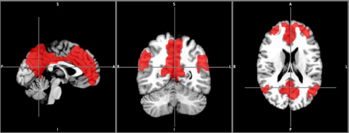
the nasal cavity. This affects the parasympathetic autonomic reflex of the central nervous system, to regulate and correct any imbalances in the nervous system that may be involved in some types of migraine [22]. Regulation of the nervous system through stimulation through the nasal cavity may explain why KOS treatment is seemingly effective for a range of debilitating conditions. Group comparison of ICA output of resting-state fMRI data, lends itself well to provide supporting evidence for this hypothesis. Since ICA is such a popular method of analysis for resting-state fMRI data, a solid knowledge of how dimensionality selection affects ICA results is vital to using ICA to conduct this group comparison study.
2.5 STUDY OUTLINE
To confidently use ICA for group comparison studies, how the selection of dimensionality affects ICA results for resting-state fMRI data must be better understood. In order to study how the selection of NIC affects ICA results, group ICA on different resting-state fMRI datasets were performed with sequentially increasing NIC from 20 – 100. Performing group ICA analysis for multiple datasets, produces a large amount of output ICs, and visually inspecting all the output ICs is very cumbersome. To facilitate the investigation, an analysis framework to automate the time consuming process of visual inspection of output ICs was developed based on Support Vector Machines (SVM) [23]. The feature-optimized classification of ICs with SVM (FOCIS) framework was implemented in a series of bash and R (https://www.r-project.org/) scripts. FOCIS was first evaluated for its performance accuracies on both single subject and group ICA results. Classification results for FOCIS was then compared against FSL-fix and manual classification results obtained through visual inspection. With favorable classification performance, FOCIS was used to automatically classify all output ICs for the different resting-state fMRI datasets at the specified range of NIC. Sub-routines within FOCIS allows for tracking individual ICs in any NIC and investigate how the specified IC changes in its time-course and spatial pattern through increasing NIC. FOCIS is also capable of tracking all output ICs in a given NIC set and compare how all the ICs change with incremental NICs. These tools allowed for better understanding of how the selection of NIC affects ICA output results. This information also provides valuable insight to how ICA should be used to perform group comparison studies.
Applying the knowledge gathered from investigating the dimensionality of resting-state fMRI datasets and how the selection of NICs affect group ICA output results, a group comparison study was conducted on migraine patients before and after KOS treatment, compared to healthy control volunteers using group ICA. The aim was to provide supporting evidence for the hypothesis for a mechanism of the KOS treatment. In addition, to be able to effectively and accurately compare sets of group ICA results, to extract differences in RFNs between patient and control groups, and before and after treatment. Group ICA were performed individually for each group for migraine patients and healthy volunteers before, during; and after KOS treatment. The results were then analyzed using the 3-way analysis of variance (ANOVA) method to detect differences between the groups, and the effect of KOS treatment.
2.6 FOCIS
The base of the FOCIS analysis framework is a classification routine aimed to automatically delineate noise and artefact ICs from those corresponding to functional connectivity networks. FOCIS is designed to obtain general information about the ICs in any given set of output ICs. Classification is performed using SVM, which is a supervised learning algorithm tailored towards binary classification. Classification features were derived from visual inspection guidelines. Potential functional connectivity network ICs should:
1. Have a t-map with activation voxels, that fulfills the voxel-wise threshold of p<0.001 and contiguous cluster size of a minimum of 20 voxels; that exhibits peak activation in cortical grey-matter; possesses little spatial overlap with known vascular, ventricular, motion, and susceptibility artefacts; and of a reasonably compact and smooth shape. 2. Have its associated time-course that reflects the expected low frequency spontaneous
fluctuations with adequate dynamic range
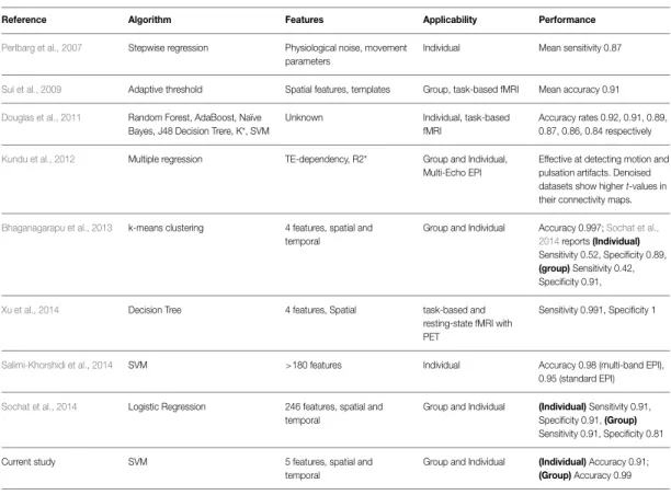
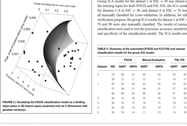
A total of 18 features were devised based on these instructions. To avoid over-fitting, only significant classifiers were chosen from the final set of features used for the classifier. Significance tests were done iteratively using a general linear model with a logit function kernel tailored to evaluate the binary classification significance. 5 of the 18 features showed to be significant at a 99% significance level. This optimization of feature selection is crucial to avoid bias and over-fitting, while retaining computational efficiency.
The ICA framework is implemented in R, using the kernlab package based on LIBSVM. Since the model cannot be expected to be linear, a non-linear SVM model was constructed using a Gaussian radial basis function kernel. Technical details concerning the implementation can be found in the relevant article [23].
2.7 ICA ANALYSIS
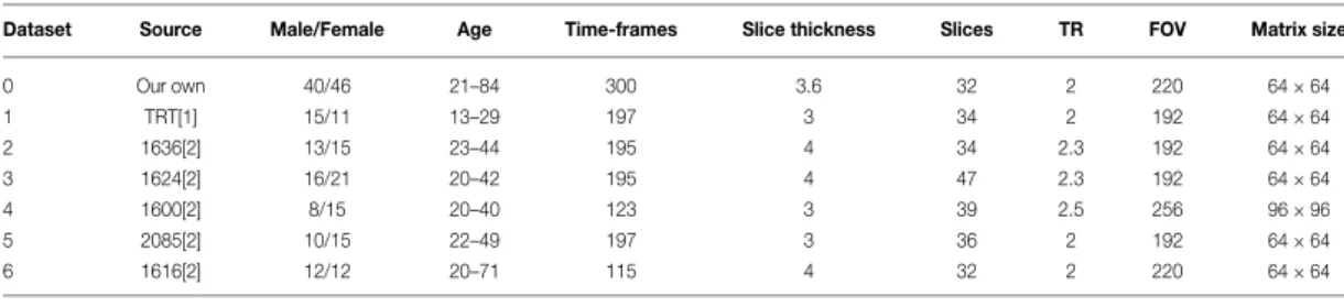
A total of 7 datasets were investigated. One dataset was acquired locally (dataset 0) and the other 6 datasets (datasets 1-6) were downloaded from the functional connectome open access database (https://www.nitrc.org/frs/?group_id=296). Consensus from multiple studies suggests that there is a relatively stable set of 10 RFNs at the level of major brain networks [6, 7, 24]. Trial runs of ICA analysis using our existing preprocessing pipeline suggests, in the worst case, the need for twice as many NICs as approximately half of the output ICs represents artefact or noise signals. Based on this information, the range of NIC was set to 20 – 100.
Group ICA was performed using the standalone melodic program in the FSL package [15, 25, 26] for different resting-state fMRI datasets ranging from 20 – 100 as the output number of ICs. 6 datasets running group ICA was investigated and a 7th dataset running single subject ICA for 5 different subjects. The datasets have differing acquisition parameters, obtained from different type of scanners, and consists of different number of subjects (details on how ICA
2.6 FOCIS
The base of the FOCIS analysis framework is a classification routine aimed to automatically delineate noise and artefact ICs from those corresponding to functional connectivity networks. FOCIS is designed to obtain general information about the ICs in any given set of output ICs. Classification is performed using SVM, which is a supervised learning algorithm tailored towards binary classification. Classification features were derived from visual inspection guidelines. Potential functional connectivity network ICs should:
1. Have a t-map with activation voxels, that fulfills the voxel-wise threshold of p<0.001 and contiguous cluster size of a minimum of 20 voxels; that exhibits peak activation in cortical grey-matter; possesses little spatial overlap with known vascular, ventricular, motion, and susceptibility artefacts; and of a reasonably compact and smooth shape. 2. Have its associated time-course that reflects the expected low frequency spontaneous
fluctuations with adequate dynamic range
A total of 18 features were devised based on these instructions. To avoid over-fitting, only significant classifiers were chosen from the final set of features used for the classifier. Significance tests were done iteratively using a general linear model with a logit function kernel tailored to evaluate the binary classification significance. 5 of the 18 features showed to be significant at a 99% significance level. This optimization of feature selection is crucial to avoid bias and over-fitting, while retaining computational efficiency.
The ICA framework is implemented in R, using the kernlab package based on LIBSVM. Since the model cannot be expected to be linear, a non-linear SVM model was constructed using a Gaussian radial basis function kernel. Technical details concerning the implementation can be found in the relevant article [23].
2.7 ICA ANALYSIS
A total of 7 datasets were investigated. One dataset was acquired locally (dataset 0) and the other 6 datasets (datasets 1-6) were downloaded from the functional connectome open access database (https://www.nitrc.org/frs/?group_id=296). Consensus from multiple studies suggests that there is a relatively stable set of 10 RFNs at the level of major brain networks [6, 7, 24]. Trial runs of ICA analysis using our existing preprocessing pipeline suggests, in the worst case, the need for twice as many NICs as approximately half of the output ICs represents artefact or noise signals. Based on this information, the range of NIC was set to 20 – 100.
Group ICA was performed using the standalone melodic program in the FSL package [15, 25, 26] for different resting-state fMRI datasets ranging from 20 – 100 as the output number of ICs. 6 datasets running group ICA was investigated and a 7th dataset running single subject ICA for 5 different subjects. The datasets have differing acquisition parameters, obtained from different type of scanners, and consists of different number of subjects (details on how ICA
analysis was performed and information on the datasets can be found in the corresponding article [23]). This process produces a great amount of ICs to investigate, more than 30000 IC time-courses with their corresponding t-maps. Without tools to partially automate the analysis process, just visually inspecting all the ICs will take a considerable amount of time.
2.8 CLASSIFICATION AND DIMENSIONALITY INVESTIGATION
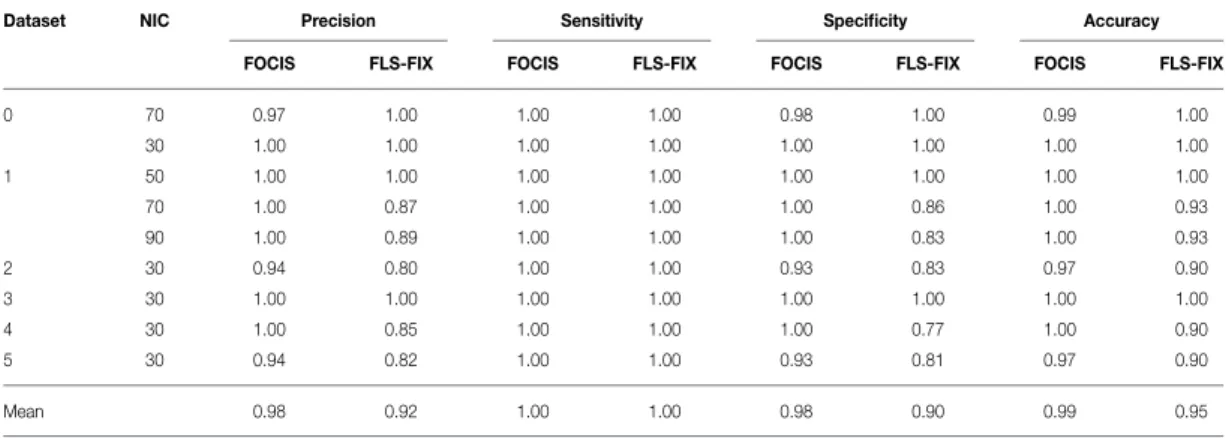
Group ICA results for dataset 1 at NIC=50, was used as training input for the classification framework. For cross evaluation, the following NIC values were used for group ICA results: NIC=30 for datasets 0-5, NIC=50 and NIC=70 for dataset 0 and NIC 70 and NIC 90 for dataset 1. Overall, FOCIS achieved 0.92 in precision, 1.00 in sensitivity and 0.98 in specificity in identifying artefact/noise ICs. All misclassifications are false negatives, where the ICs have borderline characteristics of both RFN and artefact signal contamination. Visual inspection was particularly difficult for these ICs and their “ground truth” is a matter of dispute.
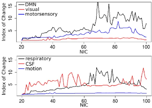
Figure 4: Index of Change for selective RFNs and artefact ICs through increasing NIC.
To quantify the changes for specific ICs, the index of change was defined based on spatial overlap and temporal association based on the ICs time course: 𝐼𝑛𝑑𝑒𝑥 𝑜𝑓 𝐶ℎ𝑎𝑛𝑔𝑒 = 1/(𝑠𝑝𝑎𝑡𝑖𝑎𝑙 𝑜𝑣𝑒𝑟𝑙𝑎𝑝 × 𝑐𝑜𝑟𝑟𝑒𝑙𝑎𝑡𝑖𝑜𝑛 𝑐𝑜𝑒𝑓𝑓𝑖𝑐𝑖𝑒𝑛𝑡 𝑜𝑓 𝐼𝐶 𝑡𝑖𝑚𝑒 𝑐𝑜𝑢𝑟𝑠𝑒), where the spatial overlap for a given IC is defined as the fraction overlap area relative to the original area of the spatial pattern given as reference. Index of Change was evaluated for well-known RFNs and
analysis was performed and information on the datasets can be found in the corresponding article [23]). This process produces a great amount of ICs to investigate, more than 30000 IC time-courses with their corresponding t-maps. Without tools to partially automate the analysis process, just visually inspecting all the ICs will take a considerable amount of time.
2.8 CLASSIFICATION AND DIMENSIONALITY INVESTIGATION
Group ICA results for dataset 1 at NIC=50, was used as training input for the classification framework. For cross evaluation, the following NIC values were used for group ICA results: NIC=30 for datasets 0-5, NIC=50 and NIC=70 for dataset 0 and NIC 70 and NIC 90 for dataset 1. Overall, FOCIS achieved 0.92 in precision, 1.00 in sensitivity and 0.98 in specificity in identifying artefact/noise ICs. All misclassifications are false negatives, where the ICs have borderline characteristics of both RFN and artefact signal contamination. Visual inspection was particularly difficult for these ICs and their “ground truth” is a matter of dispute.
Figure 4: Index of Change for selective RFNs and artefact ICs through increasing NIC.
To quantify the changes for specific ICs, the index of change was defined based on spatial overlap and temporal association based on the ICs time course: 𝐼𝑛𝑑𝑒𝑥 𝑜𝑓 𝐶ℎ𝑎𝑛𝑔𝑒 = 1/(𝑠𝑝𝑎𝑡𝑖𝑎𝑙 𝑜𝑣𝑒𝑟𝑙𝑎𝑝 × 𝑐𝑜𝑟𝑟𝑒𝑙𝑎𝑡𝑖𝑜𝑛 𝑐𝑜𝑒𝑓𝑓𝑖𝑐𝑖𝑒𝑛𝑡 𝑜𝑓 𝐼𝐶 𝑡𝑖𝑚𝑒 𝑐𝑜𝑢𝑟𝑠𝑒), where the spatial overlap for a given IC is defined as the fraction overlap area relative to the original area of the spatial pattern given as reference. Index of Change was evaluated for well-known RFNs and
artefact ICs, and irrespective of an IC being an RFN or artefact, the change of a given IC can be relatively steady or volatile (Figure 4).
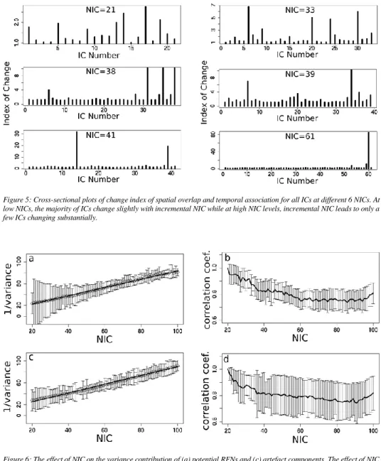
Figure 5: Cross-sectional plots of change index of spatial overlap and temporal association for all ICs at different 6 NICs. At low NICs, the majority of ICs change slightly with incremental NIC while at high NIC levels, incremental NIC leads to only a few ICs changing substantially.
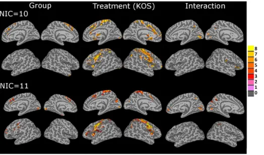
Figure 6: The effect of NIC on the variance contribution of (a) potential RFNs and (c) artefact components. The effect of NIC on the IC time-course for (b) potential RFNs and (c) artefact components.
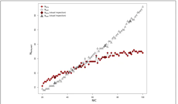
An interesting aspect to note, is the pattern for overall change of all ICs with incremental NIC. At relatively low NICs, incrementing the NIC by 1 gives rise to changes in a large fraction of all ICs. At higher NICs, a sequential increment of NIC by 1 results in major changes to only a limited number of ICs (Figure 5). This pattern can be appreciated with the variance
artefact ICs, and irrespective of an