Almost the Best of Three Worlds: Risk,
Consistency and Optional Stopping for the
Switch Criterion in Nested Model Selection
Stéphanie van der Pas∗ and Peter Grünwald∗,† e-mail:[email protected]
e-mail: [email protected]
Abstract: We study the switch distribution, introduced by Van Erven et al. (2012), applied to model selection and subsequent estimation. While switching was known to be strongly consistent, here we show that it achieves minimax optimal parametric risk rates up to alog lognfactor when comparing two nested exponential families, partially confirming a conjecture by Lauritzen (2012) and Cavanaugh (2012) that switching behaves asymptotically like the Hannan-Quinn criterion. Moreover, like Bayes factor model selection but unlike standard significance testing, when one of the models rep-resents a simple hypothesis, the switch criterion defines arobust null hypothesis test, meaning that its Type-I error probability can be bounded irrespective of the stopping rule. Hence, switching is consistent, insensitive to optional stopping and almost mini-max risk optimal, showing that, Yang’s (2005) impossibility result notwithstanding, it is possible to ‘almost’ combine the strengths of AIC and Bayes factor model selection.
Keywords and phrases: model selection, post model selection estimation, switch distribution, AIC-BIC dilemma, worst-case risk, optional stopping, consistency, expo-nential family.
1. Introduction
We consider the following standard model selection problem, where we have i.i.d. observa-tionsX1, . . . , Xn and we wish to select between two nested parametric models,
M0={pµ|µ∈M0} and M1={pµ |µ∈M1}. (1.1)
Here the Xi are random vectors taking values in some setX, M1 ⊆Rm1 for somem 1>0
and M0 = {pµ : µ ∈ M0} ⊂ M1 represents an m0-dimensional submodel of M1, where 0 ≤m0 < m1. We may thus denote M0 as the ‘simple’ and M1 as the ‘complex’ model.
We will assume that M1 is an exponential family, represented as a set of densities on X
with respect to some fixed underlying measure, so that pµ represents the density of the
observations, and we take it to be given in its mean-value parameterization. As the notation indicates, we require, without loss of generality, that the parameterizations ofM0 andM1
coincide, that is M0 ⊂ M1 is itself a set of m1-dimensional vectors, the final m1−m0
components of which are fixed to known values. We restrict ourselves to the case in which bothM1and the restriction ofM0to its firstm0components are products of open intervals.
Most model selection methods output not just a decision δ(Xn) ∈ {0,1}, but also an
indication r(Xn) ∈
R of the strength of evidence, such as a p-value or a Bayes factor. As
a result, such procedures can often be interpreted as methods for hypothesis testing, where M0represents thenull model andM1the alternative; a very simple example of our setting
is when the Xi consist of two components Xi ≡ (Xi1, Xi2), which according to M1 are
independent Gaussians whereas under M2 they can have an arbitrary bivariate Gaussian
distribution and hence can be dependent. Since we allowM0to be a singleton, this setting
also includes some very simple, classical yet important settings such as testing whether a coin is biased (M0 is the fair coin model,M1contains all Bernoulli distributions).
We consider three desirable properties of model selection methods: (a) optimal worst-case risk rate of post-model selection estimation (with risk measured in terms of squared error
∗Research supported by the Netherlands Organization for Scientific Research. †This research was supported by NWO VICI Project 639.073.04.
1
loss, squared Hellinger distance, Rényi or Kullback-Leibler divergence); (b) consistency, and, (c), for procedures which also output a strength of evidencer(Xn), whether the validity of
the evidence is insensitive to optional stopping under the null model. We evaluate the recently introduced model selection criterionδsw based on the switch distribution (Van Erven et al.,
2012) on properties (a), (b) and (c).
The switch distribution, introduced by1 Van Erven et al., (2007), was originally designed
to address the catch-up phenomenon, which occurs when the best predicting model is not the same across sample sizes. The switch distribution can be interpreted as a modification of the Bayesian predictive distribution. It also has an MDL interpretation: if one corrects standard MDL approaches (Grünwald,2007) to take into account that the best predicting method changes over time, one naturally arrives at the switch distribution. Lhéritier and Cazals (2015) describe a successful practical application for two-sample sequential testing, related to the developments in this paper but in a nonparametric context. We briefly give the definitions relevant to our setting in Section 2; for all further details we refer to Van Erven et al. (2012) andEin the Appendix.
When evaluating any model selection method, there is a well-known tension between properties (a) and (b) above: the popular AIC method (Akaike,1973) achieves the minimax optimal parametric rate of order1/nin the problem above, but is inconsistent; the same holds for the many popular model selection methods that asymptotically tend to behave like AIC, such ask-fold (for fixedk) and leave-one-out-cross-validation, the bootstrap and Mallow’s
Cp in linear regression (Efron, 1986; Shao, 1997; Stone, 1977). On the other hand, BIC
(Schwarz,1978) is consistent in the sense that for large enoughn, it will select the smallest model containing the ‘true’µ; but it misses the minimax parametric rate by a factor oflogn. The same holds for traditional Minimum Description Length (MDL) approaches (Grünwald,
2007) and Bayes factor model selection (BFMS) (Kass and Raftery, 1995), of which BIC is an approximation. This might lead one to wonder if there exists a single method that is optimal in both respects. A key result by Yang (2005) shows that this is impossible: any consistent method misses the minimax optimal rate by a factorg(n)withlimn→∞g(n) =∞.
In Section4.2we show that, Yang’s result notwithstanding, the switch distribution allows us to get very close to satisfying property (a) and (b) at the same time, at least in the problem defined above (Yang’s result was shown in a nested linear regression rather than our exponential family context, but it does hold in our exponential family setting as well; see the discussion at the end of Section3.3). We prove that in our setting, the switch model selection criterion δsw (a) misses the minimax optimal rate only by an exceedingly small
gsw(n)log lognfactor (Theorem1). Property (b), strong consistency, was already shown
by Van Erven et al. (2012). The factorgsw(n)log lognis an improvement over the extra
factor resulting from Bayes factor model selection, which has gbfms(n) logn. Indeed, as discussed in the introduction of van Erven et al. (2012), the catch-up phenomenon that the switch distribution addresses is intimately related to the rate-suboptimality of Bayesian inference. Van Erven et al. (2012) show that, while model selection based on switching is consistent, sequential prediction based on model averaging with the switching method achieves minimax optimal cumulative risk rates in general parametric and nonparametric settings, where the cumulative risk at sample sizen is obtained by summing the standard, instantaneous risk from 1 to n. In contrast, in nonparametric settings, standard Bayesian model averaging typically has a cumulative risk rate that is larger by a lognfactor. Using the cumulative risk is natural in sequential prediction settings, but Van Erven et al. (2012) left open the question of how switching would behave for the more standard, instantaneous risk. In contrast to the cumulative setting, we cannot expect to achieve the optimal rate here by Yang’s (2005) result, but it is interesting to see that switching gets so close.
We now turn to the third property, robustness to optional stopping. While consistency in the sense above is an asymptotic and even somewhat controversial notion (see Section 6), there exists a nonasymptotic property closely related to consistency that, while arguably more important in practice, has received relatively little attention in the recent statistical
1Matlab code for implementing model selection, averaging and prediction by the switch distribution is
available athttp://www.blackwellpublishing.com/rss. In general run times are comparable to those of the corresponding Bayesian methods.
literature. This is property (c) above, insensitivity to optional stopping. In statistics, the issue was thoroughly discussed, yet never completely resolved, in the 1960s; nowadays, it is viewed as a highly desirable feature of testing methods by, for example, psychologists; see (Sanborn and Hills,2014;Wagenmakers,2007). In particular, it is often argued (Wagenmakers,2007) that the fixed stopping rule required by the classical Neyman-Pearson paradigm severely and unnecessarily restricts the application domain of hypothesis testing, invalidating much of thep-values reported in the psychological literature. Approximately 55% of psychologists admitted in a survey to deciding whether to collect more data after looking at their results to see if they were significant (John et al.,2012). We analyze property (c) in terms ofrobust null hypothesis tests, formally defined in Section 5. A method defines a robust null hypothesis test if (1) it outputs evidence r(Xn) that does not depend on the stopping rule used to
determine n, and (2) (some function of) r(Xn) gives a bound on the Type-I error that
is valid no matter what this stopping rule is. Standard (Neyman-Pearson) null hypothesis testing and tests derived from AIC-type methods are not robust in this sense. For example, such tests cannot be used if the stopping rule is simply unknown, as is often the case when analyzing externally provided data — but this is just the tip of an iceberg of problems with nonrobust tests. For an exhaustive review of such problems we refer toWagenmakers(2007) who builds on, amongst others, Berger and Wolpert(1988) andPratt(1962).
Now, as first noted by Edwards et al. (1963), in simple versus composite testing (i.e. whenM0is a singleton), the output of BFMS, the Bayes factor, does provide a robust null
hypothesis test. This is one of the main reasons why for example, in psychology, Bayesian testing is becoming more and more popular (Andrews and Baguley, 2012; Dienes, 2011), even among ‘frequentist’ researchers (Sanborn and Hills, 2014). Our third result, in Sec-tion5, shows that the same holds for the switch criterion: if M0 is a singleton, so that the
problem (1.1) reduces to a simple versus composite hypothesis test, then the evidencer(Xn)
associated with the switching criterion has the desired robustness property as well and thus in this sense behaves like the Bayes factor method. The advantage, from a frequentist point of view, of switching as compared to Bayes is then that switching is a lot more sensitive: our risk rate results directly imply that the Type II error(1−power)of the switch criterion goes to0 as soon as, at sample size n, the distance between the ‘true’ distributionµ1 and
the null model, i.e.infµ∈M0kµ−µ1k 2
2 is of order (log logn)/n; for Bayes factor testing, in
order for the Type-II error to reach0, this distance must be of order(logn)/n(this was in-formally recognized byLhéritier and Cazals(2015), who reported substantially larger power of switching as compared to the Bayes factor method in a sequential two-sample testing setting).
Thus, for singleton M0, switching gives us ‘almost the best of three worlds’: minimax
rate optimality up to a log logn factor (in contrast to BFMS), consistency (in contrast to AIC-type methods) and nonasymptotic insensitivity to optional stopping (in contrast to standard Neyman-Pearson testing) in combination with a small Type-II error. For composite M0, we show in Section5 that nonasymptotic robustness to optional stopping still holds,
albeit only in a much weaker sense — thus pointing towards an obvious goal for future work, discussed in Section6: can we modify the switch distribution so as to get full optional stopping robustness also for compositeM0?
Organization This paper is organized as follows. The switch criterion is introduced in Section 2. In Section 3, we provide some preliminaries: we list the loss/risk functions for which our result holds, describe the sets in which the truth is assumed to lie, and discuss the tension between consistency and rate-optimality. Suitable post-model-selection estimators to be used in combination with the switch criterion are introduced in Section4, after which our main result on the worst-case risk of the switch criterion is stated. We also go into the relationship between the switch criterion and the Hannan-Quinn criterion in that section. In Section5we define robust null hypothesis tests, give some examples, and show that testing by switching has the desired nonasymptotic robustness to optional stopping; in constrast, AIC does not satisfy such a property at all and the Hannan-Quinn criterion only satisfies an asymptotic analogue. We also provide some simulations that illustrate our results. Section6
Appendix.
Notations and Conventions We use xn = x
1, . . . , xn to denote n observations, each
taking values in a sample spaceX. For a set of parameters M, µ∈M, andx∈ X, pµ(x)
invariably denotes the density or mass function of x under the distribution Pµ of random
variable X, taking values inX. This is extended to n outcomes by independence, so that
pµ(xn) :=Q n
i=1pµ(xi)and Pµ(Xn ∈An), abbreviated toPµ(An), denotes the probability
thatXn ∈AnforXn=X1, . . . , Xni.i.d.∼Pµ. Similarly,Eµdenotes expectation underPµ.
As is customary, we writean bn to denote0<limn→∞infan/bn ≤limn→∞supan/bn <
∞. For notational simplicity we assume throughtout this paper that whenever we refer to a sample sizen, thenn≥3 to ensure thatlog lognis defined and positive.
Throughout the text, we refer to standard properties of exponential families without always giving an explicit reference; all desired properties can be found, in precise form, in (Barndorff-Nielsen, 1978) and, on a less formal level, in (Grünwald,2007, Chapter 18,19).
2. Model Selection by Switching
The switch distribution (Van Erven et al., 2007; 2012) is a modification of the Bayesian predictive distribution, inspired by Dawid’s (1984) ‘prequential’ approach to statistics and the relatedMinimum Description Length (MDL) Principle (Barron et al.,1998;Grünwald,
2007). The correspondingswitch criterioncan be thought of as Bayes factor model selection with a prior on meta-models, where each meta-model consists of a sequence of basic models and associated starting times: until timet1, follow modelk1, from timet1tot2, follow model
k2, and so on. The fact that we only need to select between two nested parametric models
allows us to considerably simplify the set-up of Van Erven et al. (2012), who dealt with countably infinite sets of arbitrary models.
It is convenient to directly introduce the switch criterion as a modification of the Bayes factor model selection (BFMS). Assuming equal prior 1/2 on each of the models M0 and
M1, BFMS associates each modelMk,k∈ {0,1}, with amarginal distribution pB,k with pB,k(xn) :=
Z
µ∈Mk
ωk(µ)pµ(xn)dµ, (2.1)
where ωk is a prior density on Mk. It then selects model M1 if and only if pB,1(xn) >
pB,0(xn).
The basic idea behind MDL model selection is to generalize this in the sense that each model Mk is associated with some ‘universal’ distribution pU,k; one then picks the k for
whichpU,k(xn)is largest.pU,k may be set to the Bayesian marginal distribution, but other
choices may be preferable in some situations. Switching is an instance of this; in our simplified setting, it amounts to associatingM0with a Bayes marginal distributonpB,0as before.pU,1
however is set to the switch distribution psw,1. This distribution corresponds to a switch
between modelsM0 andM1 at some sample points, which is itself uncertain; before point
s, the data are modelled as coming from M0, usingpB,0; after points, they are modelled
as coming from M1, using pB,1. Formally, we denote the strategy that switches from the
simple to the complex model aftertobservations byp¯t;psw,1 is then defined as the marginal
distribution by averagingp¯tovert, with some probability mass functionπ(analogous to a
Bayesian prior) overt∈ {1,2, . . .}:
¯ pt(xn) =pB,0(xt−1)·pB,1(xt, . . . , xn |xt−1) psw,1(xn) = ∞ X t=1 π(t)¯pt(xn),
where switching at t = 1 corresponds to predicting with pB,1 at each data point, and
switching at any t > nto predicting with pB,0. We remind the reader that even for i.i.d.
learns from data. The model selection criterionδsw mapping sequences of arbitrary length
tok∈ {0,1}is then defined, for each n, as follows:
δsw(xn) = 0 if psw,1(x n) pB, 0(xn) ≤1 1 if psw,1(x n) pB, 0(xn) >1 . (2.2)
When definingpsw,1it is sufficient to consider switching times that are equal to a power of
two. Thus, we restrict attention to ‘priors’πon switching time with support on20,21,22, . . .. For our subsequent results to hold, π should be such that π(2i) decays like i−κ for some
κ >1. An example of such a prior withκ= 2isπ(2i) = 1/((i+ 1)(i+ 2)),π(j) = 0for any j that is not a power of 2.
To prepare for Theorem1, we instantiate the switch criterion to the problem (1.1). We define pB,1 as any distribution of the form (2.1) whereω1 is a continuous prior density on
M1 that is strictly positive on all µ∈M1. To define pB,0 we need to take a slight detour,
because we parameterizedM0in terms of anM0 that has a fixed value on its finalm1−m0
components: it is an m0-dimensional family with an m1-dimensional parameterization, so
one cannot easily express a prior onM0as a density onM0. To overcome this, we distinguish
between the case that m0= 0 and m0>0. In the former caseM0 has a single element ν,
and we define pB,0 = pν. In the latter case, we define Π00 : M0 → Rm0 as the projection
of µ ∈ M0 on its first m0 components, and Π00(M0) := {Π00(µ) : µ ∈ M0}. For µ ∈ M0,
we definepΠ0
0(µ)=pµ, and we then letω0be a continuous strictly positive prior density on Π00(M0), and we definepB,0(xn) :=
R µ0∈Π0
0(M0)
ω0(µ0)pµ0(xn)dµ0.
Two important remarks are in order: first, the fact that we associateM1with a
distribu-tion incorporating a ‘switch’ fromM0toM1does not meanthat we really believe that data
were sampled, until some pointt, according toM0and afterwards according toM1. Rather,
it is suggested by prequential and MDL considerations, which suggest that one should pick the model that performs best in sequentially predicting data; and if the data are sampled from a distribution in M1 that is not in M0, but quite close to it in KL divergence, then
pB,1is suboptimal for sequential prediction, and can be substantially outperformed bypsw,1.
This is explained at length by Van Erven et al. (2012), and Figure 1 in that paper especially illustrates the point. The same paper also explains how one can use dynamic programming to arrive at an implementation that has the same computational efficiency as computation of the standard Bayes model selection decision.
Second, the criterion (2.2) as defined here is not 100% equivalent to the special case of the construction of Van Erven et al. (2012) specialized to two models, but rather a simplification thereof. We do this purely for ease of explanation: varying the exponentκin the priorπ(2i)∝i−κ defined above — which is a free parameter of the switch distribution — has a stronger effect on the switch criterion than switching between the two versions of the switch distribution. This is explained in the Appendix, where we also explain why all our results continue to hold if we were to follow the original construction; conversely, the strong consistency result for the construction of Van Erven et al. (2012) trivially continues to hold for the criterion (2.2) used in the present paper.
3. Rate-optimality of post-model selection estimators
This section contains some background to our main result, Theorem1. In Section3.1, we first list the loss functions for which our main result holds, and define the CINECSI sets in which the truth assumed to lie. We then discuss the minimax parametric risk for our model selection problem in Section3.2. This section ends with a discussion on the generality of the impossibility result ofYang (2005) in Section3.3.
3.1. Loss functions and CINECSI sets
LetM={pµ |µ∈M} be an exponential family given in its mean-value parameterization
some m > 0; see the Appendix for a formal definition of exponential families and mean-value parameterizations. Note that we do not require the family to be ‘full’; for example, the Bernoulli model with success probabilityµ∈M1 = (0.2,0.4) counts as an exponential
family in our (standard) definition.
Suppose that we measure the quality of a densitypµ0 as an approximation topµ by a loss
functionL:M ×M →R. The standard definition of the (instantaneous) risk of estimator ˘
µ : S i>0X
i → M at sample size n, as defined relative to loss L, is given by its expected
loss,
R(µ,µ, n˘ ) =Eµ[L(µ,µ˘(Xn))],
whereEµ denotes expectation overX1, . . . , Xn i.i.d. ∼Pµ. Popular loss functions are:
1. Thesquared error loss:dSQ(µ0, µ) =kµ0−µk22;
2. The standardized squared error loss which is a version of the squared Mahalonobis distance, defined as
dST(µ0kµ) := (µ−µ0)TI(µ0)(µ−µ0), (3.1)
where T denotes transpose,I(·)is the Fisher information matrix, and we viewµand
µ0 as column vectors;
3. The Rényi divergence of order1/2, defined as
dR(µ0, µ) =−2 logEµ0 h (pµ(X)/pµ0(X)) 1 2 i ;
4. The squared Hellinger distancedH2(µ0, µ) = 2
1− Eµ0 h (pµ(X)/pµ0(X)) 1 2 i ; 5. The KL (Kullback-Leibler) divergenceD(pµ0kpµ), henceforth abbreviated toD(µ0kµ).
We note that there is a direct relationship between the Rényi divergence and squared Hellinger distance:
dH2(µ0, µ) = 2
1−e−dR(µ0,µ)/2. (3.2)
In fact, as we show below, these loss functions are all equivalent (equal up to universal constants) on CINECSI sets. Such sets will play an important role in the sequel. They are defined as follows:
Definition 1 (CINECSI). A CINECSI (Connected, Interior-Non-Empty-Compact-Subset-of-Interior) subsetof a setM is a connected subset of the interior ofM that is itself compact and has nonempty interior.
The following proposition is proved in the Appendix.
Proposition 1. LetM be the mean-value parameter space of an exponential family as above, and letM0be a CINECSI subset ofM. Then there exist positive constantsc1, c2, . . . , c6 such
that for all µ, µ0∈M0,
c1kµ0−µk22≤c2·dST(µ0kµ)≤dH2(µ0, µ)≤dR(µ0, µ)≤D(µ0kµ)≤c3kµ0−µk22. (3.3)
and for allµ0 ∈M0, µ∈M (i.e.µis now not restricted to lie inM0),
dH2(µ0, µ)≤c4kµ0−µk22≤c5·dST(µ0kµ)≤c6kµ0−µk22. (3.4)
CINECSI subsets are a variation on the INECCSI sets of (Grünwald, 2007). Our main result, Theorem 1, holds for all of the above loss functions, and for general ‘sufficiently efficient’ estimators. While the equivalence of the losses above on CINECSI sets is a great help in the proofs, we emphasize that we never require these estimators to be restricted to CINECSI subsets of M — although, since we require M to be open, every ‘true’ µ ∈ M
will lie insomeCINECSI subsetM0 ofM, a statistician who employs the modelMcannot know what thisM0 is, so such a requirement would be unreasonably strong.
3.2. Minimax parametric risk
We say that a quantityfn converges at rategn if fn gn. We say that an estimator µ˘ is
minimax-rate optimal relative to a modelM={pµ|µ∈M}restricted to a subsetM0⊂M
if
sup µ∈M0
R(µ,µ, n˘ )
converges at the same rate as
inf ˙ µ µsup∈M0
R(µ,µ, n˙ ), (3.5)
where µ˙ ranges over all estimators ofµat sample size n, that is, all measurable functions fromXn to M.
For parametric models, the minimax risk (3.5) is typically of order 1/n when R is de-fined relative to any of the loss measures dede-fined in Section 3.1 and M0 is an arbitrary
CINECSI subset of M (Van der Vaart, 1998) — models for which this holds include e.g. most location families and all curved exponential families, which include as a special case all standard exponential families. For this reason, from now on we refer to 1/n as the minimax parametric rate. Note that, crucially, the restriction µ ∈M0 is imposed only on the data-generating distribution, not on the estimators, and, since we will require models with open parameter sets M such that for every δ > 0, there is a CINECSI subset Mδ0
of M with supµ∈Minfµ0∈M0
δkµ−µ
0||2
2 < δ, every possible µ ∈ M will also lie in some
CINECSI subset Mδ0 that ‘nearly’ covers Mδ. This makes the restriction to CINECSI M0
in the definition above a mild one. Still, it is necessary: at least for the squared error loss, for most exponential families (the exception being the Gaussian location family), we have
infµ˙supµ∈M0
δR(µ,µ, n˙ ) = Cδ/n for some constant Cδ > 0, but the smallest constant for
which this holds may grow arbitrarily large asδ→0, the reason being that the determinant of the Fisher information may tend to0or ∞asδ→0.
Now consider a model selection criterion δ : S i>0X
i → {0,1, . . . , K−1} that selects,
for given data xn of arbitrary length n, one of a finite number K of parametric models
M0, . . . ,MK−1 with respective parameter sets M0, . . . , MK−1. One way to evaluate the
quality ofδis to consider the risk attained after first selecting a model and then estimating the parameter vector µ using an estimatorµ˘k associated with each model Mk. This
post-model selection estimator (Leeb and Pötscher, 2005) will be denoted by µ˘˘k(xn), where ˘k
is the index of the model selected by δ. The risk of a model selection criterion δ is thus
R(µ, δ, n) = EµL(µ,µ˘˘k(Xn)), where L is a given loss function, and its worst-case risk
relative to µrestricted toMk0 ⊂Mk is given by sup µ∈M0 k R(µ, δ, n) = sup µ∈M0 k EµL(µ,µ˘˘k(Xn)). (3.6)
We are now ready to define what it means for a model selection criterion to achieve the minimax parametric rate.
Definition 2. A model selection criterionδ achieves the minimax parametric rate if there exist estimators µ˘k, one for each Mk under consideration, such that, for every CINECSI
subsetMk0 ofM:
sup µ∈M0
k
R(µ, δ, n)1/n.
Just as in the fixed-model case, the restriction µ ∈ Mk0 is imposed only on the data-generating distribution, not on the estimators.
3.3. The result of Yang (2005) transplanted to our setting
In this paper, as stated in the introduction, we further specialize the setting above to problem (1.1) where we select between two nested exponential families, which we shall always assume to be given in their mean-value parameterization. To be precise, the ‘complex’ model M1
vectorµ, and the ‘simple’ modelM0contains distributions with the same parametrization,
where the finalm1−m0 components are fixed to valuesνm0+1, . . . , νm1. We introduce some
notation to deal with the assumption that M1 and its restriction of M0 to its first m0
components are products of open intervals. Formally, we require thatM1andM0are of the
form
M1= (ζ1,1, η1,1)×. . .×(ζ1,m1, η1,m1)
M0= (ζ0,1, η0,1)×. . .×(ζ0,m0, η0,m0)× {νm0+1} ×. . .× {νm1} (3.7)
where, for j = 1, . . . , m0, we have −∞ ≤ ζ1,j ≤ ζ0,j < η0,j ≤ η1,j ≤ ∞; and for j = m0+ 1, . . . , m1, we have−∞ ≤ζ1,j < νj < η1,j ≤ ∞.
For example, M1 could contain all normal distributions with meanµ and varianceσ2,
with mean value parametersµ1=µ2+σ2andµ2=µ, andM1= (0,∞)×(−∞,∞), while
M0 could contain all normal distributions with mean zero and unknown variance σ2, so
M0= (0,∞)× {0}.
Yang(2005) showed in a linear regression context that a model selection criterion cannot both achieve the minimax optimal parametric rate and be consistent; a practitioner is thus forced to choose between a rate-optimal method such as AIC and a consistent method such as BIC. Inequality (3.9) below provides some insight into why this AIC-BIC dilemma can occur. A similar inequality appears in Yang’s paper for his linear regression context, but it is still valid in our exponential family setting, and the derivation — which we now give — is essentially equivalent.
To state the inequality, we need to relateµ1∈M1to a component inM0. For any given
µ1= (µ1,1, . . . , µ1,m1) T ∈M
1, we will define
Π0(µ1) := (µ1,1, . . . , µ1,m0, νm0+1, . . . , νm1)
T (3.8)
to be theprojection ofµ1 onM0. The difference betweenΠ0 of (3.8) andΠ00 in Section2is
thatΠ0 is a function fromRm1 to
Rm1, whereasΠ0
0is a function fromR m1 to
Rm0;Π 0(µ1)
andΠ00(µ1)agree in the firstm0components. Note thatΠ0(µ1)obviously minimizes, among
allµ∈M0, the squared Euclidean distancekµ−µ1k22topµ1; somewhat less obviously it also
minimizes, amongµ∈M0, the KL divergenceD(pµ1kpµ)(Grünwald,2007, Chapter 19); we
may thus think of it as the ‘best’ approximation of the ‘true’µ1 withinM0; we will usually
abbreviateΠ0(µ1)toµ0.
Let An be the event that the complex model is selected at sample size n. Since M1 is
an exponential family, the MLE bµ1 is unbiased and µb0 coincides with µb1 in the first m0
components, so thatEµ1[µ0−µb0(X
n)] = 0, and hence we can rewrite, for anyµ
1∈M1, the
squared error risk as
R(µ1, δ, n) =Eµ1 1Ankµ1−µb1(X n)k2 2+1Ac nkµ1−bµ0(X n)k2 2 =Eµ1 1Ankµ1−µb1(X n)k2 2+1Ac nkµ0−bµ0(X n)k2 2+ 1Ac nkµ1−µ0k 2 2 ≤Eµ1 kµ1−µb1(X n)k2 2+kµ0−µb0(X n)k2 2 +P(Acn)kµ1−µ0k22 ≤2R(µ1,bµ1, n) +P(Acn)kµ1−µ0k22. (3.9)
The first part of the proof of our main result, Theorem 1, extends this decomposition to general estimators and loss functions.
The first term on the right of (3.9) is of order 1/n. The second term depends on the ‘Type-II error’, i.e. the probability of selecting the simple model when it is not actually true. A low worst-case risk is attained if this probability is small, even if the true parameter is close to µ0. This does leave the possibility for a risk-optimal model selection criterion to
incorrectly select the complex model with high probability. In other words, a risk-optimal model selection method may not be consistent if the simple model is correct. The theorem byYang (2005), arguing from decomposition (3.9), essentially demonstrates that it cannot be. Due to the general nature of (3.9), it seems likely that his result holds in much more general settings: a procedure attains a low worst-case risk by selecting the complex model with high probability, which is excellent if the complex model is indeed true, but leads to
inconsistency if the simple model is correct. Indeed, we have shown in earlier work that the dilemma is not restricted to linear regression, but occurs in our exponential family problem (1.1) as well as long asM0={ν}is a singleton (see (Van der Pas,2013) for the proof, which
is a simple adaptation of Yang’s proof that, we suspect, can be extended to nonsingleton M0as well). Hence, as the switch criterion is strongly consistent (Van Erven et al. (2012)),
we know that the worst-case risk rate of the switch criterion cannot be of the order1/n in general.
4. Main result
We perform model selection by using the switch criterion, as specified in Section2. After the model selection, we estimate the underlying parameterµ. We discuss post-model selection estimators suitable to our problem in Section 4.1. We are then ready to present our main result, Theorem 1 in Section 4.2, stating that the worst-case risk for the switch criterion under the loss functions listed in Section 3.1 attains the minimax parametric rate up to a
log lognfactor.
4.1. Post-model selection: sufficiently efficient estimators
Our goal is to determine the worst-case rate for the switch criterion applied to two nested exponential families, which we combine with an estimator as follows: if the simple model is selected, µ will be estimated by an estimator µ˘0 with range M0. If the complex model is
selected, the estimate of µ will be provided by another estimator µ˘1 with range M1. Our
result will hold for all estimatorsµ˘0 andµ˘1 that aresufficiently efficient:
Definition 3 (sufficiently efficient). The estimators{µ˘k→Mk|k∈ {0,1}}aresufficiently
efficient with respect to a divergence measuredgen(·k·)if (withµ0= Π0(µ1)as in (3.8)), for
every CINECSI subsetM10 ofM1, there exists a constantC >0such that for alln, sup µ1∈M0 1 Eµ1[dgen(µ0kµ˘0)]≤C· sup µ1∈M0 1 Eµ1[dgen(µ1kµ˘1)]≤ C n. (4.1)
Note that this is a stronger requirement than just rate-optimality: we additionally re-quire that, if the estimate µ˘0 is used on data sampled from µ1 ∈M1 (‘misspecification’),
then still µ˘0 converges to µ0, the best approximation of µ1 within M0 at rate O(1/n). In
the Appendix we provide a detailed discussion of sufficiently efficient estimators by means of several examples. In a nutshell, it turns out that for (standardized) squared error and Hellinger distance, the MLE is either sufficiently efficient (e.g. for the Gaussian and gamma families), or can be made sufficiently efficient by trivial modifications. For the same losses, Bayes MAP estimates based on proper priors are sufficiently efficient without modification for nearly all exponential families. For Rényi and KL divergences, MLEs can sometimes be problematic but Bayes MAP estimators are still usually sufficiently efficient.
4.2. Main result: risk of the switch criterion
We now present our main result, which states that for the exponential family problem under consideration, the worst-case instantaneous risk rate ofδsw is of order (log logn)/n.
Hence, the worst-case instantaneous risk ofδswis very close to the lower bound of1/n, while
the criterion still maintains consistency.
The theorem holds for any of the loss functions listed in Section 3.1. We denote this by using the generic loss function dgen, which can be one of the following loss functions:
squared error loss, standardized squared error los, KL divergence, Rényi divergence of order 1/2, or squared Hellinger distance. Apart from the sufficiently efficient condition onµ˘0and ˘
µ1, there are two minor conditions on the priors used in defining the switch distribution:
prior normally considered for exponential family inference. Assumption 3 requires that the prior probability of switching at time t = 2i is strictly decreasing and not exponentially
small in i. Since these priors are user-defined and not dependent on the underlying true distribution, these conditions can easily be satisfied in practice.
Theorem 1. Let M0 = {pµ | µ ∈ M0} and M1 = {pµ | µ ∈ M1} be nested
exponen-tial families in their mean-value parameterization, where M0 ⊆ M1 are of the form (3.7).
Assume:
1. µ˘0 and µ˘1 are sufficiently efficient estimators relative to the chosen lossdgen;
2. δsw is constructed withpB,0andpB,1 defined as in Section2with priorsωk that admit
a strictly positive, continuous density;
3. andpsw,1is defined relative to a prior πwith support on{0,1,2,4,8, . . .} andπ(2i)∝
i−κ for someκ >1.
Then for every CINECSI subset M10 of M1, we have: sup µ1∈M0 1 R(µ1, δsw, n) =O log logn n ,
forR(µ, δsw, n)the risk at sample size ndefined relative to the chosen loss dgen.
Example 1. [Our Setting vs. Yang’s]Yang(2005) considers model selection between two nested linear regression models with fixed design, where the errors are Gaussian with fixed variance. The risk is measured as the in-model squared error risk (‘in-model’ means that the loss is measured conditional on a randomly chosen design point that already appeared in the training sample). Within this context he shows that every model selection criterion that is (weakly) consistent cannot achieve the 1/n minimax rate. The exponential family result above leads one to conjecture that the switch distribution achieves O((log logn)/n)
risk in Yang’s setting as well. We suspect that this is so, but actually showing this would require substantial additional work. Compared to our setting, Yang’s setting is easier in some and harder in other respects: under the fixed-variance, fixed design regression model, the Fisher information is constant, making asymptotic results hold nonasymptotically, which would greatly facilitate our proofs (and obliterate any need to consider CINECSI sets or undefined MLE’s). On the other hand, evaluating the risk conditional on a design point is not something that can be directly embedded in our proofs.
Example 2. [Switching vs. Hannan-Quinn] In their comments on Van Erven et al. (2012),Lauritzen(2012) andCavanaugh(2012) suggested a relationship between the switch model selection criterion and the criterion due toHannan and Quinn(1979). For the expo-nential family models under consideration, the Hannan-Quinn criterion with parameter c, denoted as HQ, selects the simple model, i.e.δHQ(xn) = 0, if
−logp b µ0(x n)< −logp b µ1(x n) +clog logn,
and the complex model otherwise. In their paper, Hannan and Quinn show that this criterion is strongly consistent forc >1.
As shown byBarron et al.(1999), under some regularity conditions, penalized maximum likelihood criteria achieve worst-case quadratic risk of the order of their penalty divided by n. One can show (details omitted) that this is also the case in our specific setting and hence, that the worst-case risk rate of HQ for our problem is of order(log logn)/n. Our main result, Theorem1, shows that the same risk rate is achieved by the switch distribution, thus partially confirming the conjecture ofLauritzen(2012) andCavanaugh(2012): HQ achieves the same risk rate as the switch distribution and, for the right choice of c, is also strongly consistent. This suggests that the switch distribution and HQ, at least for some specific value c0, may behave asymptotically indistinguishably. The earlier results of Van der Pas
(2013) suggest that this is indeed the case if M0 is a singleton; if M0 has dimensionality
larger than 0, this appears to be a difficult question which we will not attempt to resolve here — in this sense the conjecture ofLauritzen(2012) andCavanaugh(2012) has only been partially resolved.
Because HQ and δsw have been shown to be both strongly consistent and achieve the
same rates for this problem, one may wonder whether one criterion is to be preferred over the other. For this parametric problem, HQ has the advantage of being simpler to analyze and implement. The criterionδsw can however, be used to define a robust hypothesis test
as in Section 5 below. As we shall see there, HQ is insensitive to optional stopping in an asymptotic sense only, whereas robust tests such as the switch criterion are insensitive to optional stopping in a much stronger, nonasymptotic sense. Except for the normal location model, for which the asymptotics are precise, the HQ criterion cannot be easily adapted to define such a robust, nonasymptotic test. Another advantage of switching is that it can be combined with arbitrary priors and applied much more generally, for example when the constituting models are themselves nonparametric (Lhéritier and Cazals,2015), are so irregular that standard asymptotics such as the law of the iterated logarithm are no longer valid, or are represented by black-box predictors such that ML estimators and the like cannot be calculated. In all of these cases the switch criterion can still be defined and — given the explanation in the introduction of Van Erven et al. (2012) — one may still expect it to perform well.
5. Robust null hypothesis tests
Bayes factor model selection, the switch criterion, AIC, BIC, HQ and most model selection methods used in practice are really based on thresholding the output of a more informative model comparison method. This is defined as a function from data of arbitrary size to the nonnegative reals. Given data xn, it outputs a number r(xn) between 0 and ∞ that is a deterministic function of the dataxn. Every model comparison methodrand thresholdthas an associated model selection method δr,t that outputs 1 (corresponding to selecting model
M1) ifr(xn) ≤t, and 0 otherwise. As explained below, such model comparison methods
can often be viewed as performing a null hypothesis test withM0 the null hypothesis,M1
the alternative hypothesis andt akin to a significance level.
Example 1 (BFMS): The output of the Bayes factor model comparison method is the posterior odds ratio rBayes(xn) = P(M0|xn)/P(M1|xn). The associated model selection
method (BFMS) with thresholdt selects model M1 if and onlyrBayes(xn)≤t. Example 2 (AIC): Standard AIC selects modelM1 iflog(pµb1(x
n)/p b µ0(x
n))> m 1−m0.
We may however consider more conservative versions of AIC that only selectM1 if log(p b µ1(x n)/p b µ0(x n))−(m 1−m0)≥ −logt. (5.1)
We may thus think of AIC as a model comparison method that outputs the left-hand side of (5.1), and that becomes a model selection method when supplied with a particulart.
Now classical Neyman-Pearson null hypothesis testing requires the sampling plan, or equivalently, the stopping rule, to be determined in advance to ensure the validity of the subsequent inference. In the important special case of (generalized) likelihood ratio tests, this even means that the sample sizenhas to be fixed in advance. In practice, greater flexibility in choosing the sample sizenis desirable (Wagenmakers(2007) provides sophisticated examples and discussion). Below, we discuss hypothesis tests that allow such flexibility by virtue of the property that their Type I-error probability remains bounded irrespective of the stopping rule used. Theserobust null hypothesis tests are defined below. As will be shown, whenever the null hypothesisM0 ={pµ0} is ‘simple’, i.e. a singleton (simple vs. composite testing),
both Bayes factor model selection (BFMS) and the switch distribution define such robust null hypothesis tests, whereas AIC does not and HQ does so only in an asymptotic sense. As we argue in Section5.3, the advantage of switching over BFMS is then that, while both share the robustness Type-I error property, switching has significantly smaller Type-II error (larger power) than BFMS when the ‘truth’ is close to M0, which is a direct consequence
of it having a smaller risk under the alternative M1. To make this point concrete, and
to indicate what may happen if M0 is not a singleton, we provide a simulation study in
5.1. Bayes Factors with singleton M0 are Robust under Optional Stopping
In many cases, for each 0 < α < 1 there is an associated threshold t(α), which is a strictly increasing function of α, such that for every t ≤ t(α) we have that δr,t becomes
a null hypothesis significance test (NHST) with type-I error probability bounded by α. In particular, then δr,t(α) is a standard NHST with type-I error bounded byα. For example,
for AIC withM0 ={0} and M1 =R representing the normal family of distributions with
unit variance, we may select t(α) = exp(−2/zα/2 2), wherezα/2 is the upper (α/2)-quantile
of the standard normal distribution. This results in the generalized likelihood ratio test at significance levelα.
We say that model comparison method r defines a robust null hypothesis test for null hypothesisM0if for all µ0∈M0, all0≤α≤1,
Pµ0(∃n:δr,t(α) (X
n) = 1)≤α. (5.2)
Hence, a test that satisfies (5.2) is a valid NHST test at each fixed significance levelα, inde-pendently of the stopping rule used. If a researcher can obtain a maximum ofnobservations, the probability of incorrectly selecting the complex model will remain bounded away from one, regardless of the actual number of observations made.
It is well-known that Bayes factor model selection provides a robust null hypothesis test if we set t(α) =α, as long as M0 is a singleton. In other words, we may view the output
of BFMS as a ‘robust’ variation of the p-value. This was already noted by Edwards et al.
(1963) and interpreted as a frequentist justification for BFMS; it also follows immediately from the following result.
Theorem 2 (Special Case of Eq. (2) of Shafer et al. (2011)). Let M0,M1, M0 and M1
be as in Theorem 1with common support X ⊂Rd for some d >0. Let(X1, X2, . . .) be an
infinite sequence of random vectors all with support X, and fix two distributions,P0¯ and¯P1 onX∞ (so that under both ¯
P0 andP1¯ ,(X1, X2, . . .)constitutes a random process). Let, for
each n, p¯(jn) represent the marginal density of (X1, . . . , Xn) for the first n outcomes under
distributionP¯j, relative to some product measureρn on (Rd)n (we assumeP0¯ andP1¯ to be
such that these densities exist). Then for all α≥0,
¯ P0 ∃n: p¯ (n) 0 (X n) ¯ p(1n)(Xn) ≤α ! ≤α.
We first apply this result for Bayes factor model selection, with model priorsπ0=π1 = 1/2, so thatrBayes(xn) =P(M0|xn)/P(M1|xn) =pB,0(xn)/pB,1(xn). We immediately see: Corollary 1. If M0 = {µ0} represents a singleton null model, then pB,0 = pµ0 so that,
applying Theorem2withPB,0=Pµ0, we see from (5.2) that, if we sett(α) =α, then Bayes
factor model selection constitutes a robust hypothesis test for null hypothesis M0.
What happens ifM0 is not singleton? Full robustness would require that (5.2) holds for
allµ0∈M0. The simulations below show that this will in general not be the case for Bayes
factor model selection. Yet, the same reasoning as used in Corollary1 implies that we still have some type of robustness in a much weaker sense, which one might call “robustness in prior expectation” relative to priorω0onM0. Namely, we have for all0≤α≤1:
PB,0(∃n:δr,t(α) (Xn) = 1)≤α, (5.3)
wherePB,0is the Bayes marginal distribution under priorω0. In other words, if the beliefs
of a Bayesian who adopts prior ω0 on model M0 were accurate, then the BFMS method
would still give robust p-values, independently of the stopping rule. While for a subjective Bayesian, such a weak form of robustness might perhaps still be acceptable, we will stick to the stronger definition instead, equating ‘robust hypothesis tests’ with tests satisfying (5.3) uniformly for allµ0∈M0.
Remark In practice we may very well be interested in a significance level αn that is a
fixed function of the sample size n, i.e., given data Xn, we choose M
1 iff the output of
the model comparison method is larger thant(αn). Both Bayesian and switch-based model
comparison may be used in this manner, and Theorem2still holds withαreplaced byαn;
we focus on the fixedαcase for simplicity only.
5.2. AIC is not, and HQ is only Asymptotically Robust
The situation for AIC is quite different from that for BFMS and switching: for every function
t: (0,1)→R>0, we have, even for everysingle0< α <1, thatδAIC,t(α)isnot a robust null
hypothesis test for significance levelα. Hence AIC cannot be transformed into a robust test in this sense. This can immediately be seen when comparing a 0-dimensional (fixed mean
µ0) with a 1-dimensional Gaussian location familyM1 (extension to general multivariate
exponential families is straightforward but involves tedious manipulations with the Fisher information). Evaluating the left hand side of (5.1) yields that δAIC,t(α) will select the
complex model if n X i=1 ˜ Xi ≥ √ 2n t(α), (5.4)
where theX˜i are variables with mean 0 and variance 1 if M0 is correct. Hence, as a
con-sequence of the law of the iterated logarithm (see for example Van der Vaart (1998)), with probability one, infinitely manynexist such that the complex model will be favored, even though it is incorrect.
It is instructive to compare this to the HQ criterion, which, in this example, using the same notation as in (5.4), selects the complex model if
n X i=1 ˜ Xi ≥p2cnlog logn.
Ifc >1(the case in which HQ is strongly consistent), then this inequality will almost surely not hold for infinitely many n, as again follows from the law of the iterated logarithm. The reasoning can again be extended to other exponential families, and we find that the HQ criterion with c >1 is robust to optional stopping in the crude, asymptotic sense that the probability that there exist infinitely many sample sizes such that the simple model is incorrectly rejected is zero. Yet HQ does not define a robust hypothesis test in the sense above: to get the numerically precise Type I-error bound (5.2) we would need to definet(α)
in a model-and sample-size-dependent manner, which is quite complicated in all cases except the Gaussian location families where the asymptotics hold precisely. We note that the same type of asymptotic robustness holds for the BIC criterion as well.
5.3. Switching with singleton M0 is Robust under Optional Stopping
The main insight of this section is simply that, just like BFMS, switching can be used as a robust null hypothesis test as well, as long asM0is a singleton: we can view the switch
distri-bution as a model comparison method that outputs odds ratiorsw(xn) =pB,0(xn)/psw,1(xn).
Until now, we used it to select model 1 ifrsw(xn)≤1. If instead we fix a significance levelα
and select model 1ifrsw(xn)≤α, then we immediately see, by applying Theorem2 in the
same way as for the Bayes factor case, thatrsw constitutes a robust null hypothesis test as
long as M0 is a singleton model (of course, if we selectM1 as soon as rsw outputs t≤α,
thenαis merely an upper bound on the Type-I error; the actual value might even be lower, as illustrated in the simulations below). Similarly – at least if the priors involved in the switch criterion are chosen independently of the stopping rule — just like BFMS, the result
rsw(xn)of model comparison by switching does not depend on the ‘sampling intentions’ of
— at least for singletonM0. Yet, from a frequentist perspective, switching is preferable to
BFMS, since it has substantially better power (type-II error) properties. As could already be seen from Yang’s decomposition (3.9), there is an intimate connection between Type-II error and the risk rate achieved by any model comparison method. Formally, we have the follow-ing result, a direct corollary of Theorem4of the Appendix, which is itself a major building block of our main result Theorem1 (plug inγ=α−1into (D.3) to get the corollary):
Corollary 2. Using the same notations and under the same conditions as Theorem 1, for anyα >0, there exist constantsC1, C2>0 such that, for every CINECSI subsetM10 of M1,
for every sequence µ(1)1 , µ(2)1 , . . . of elements of M0
1 with for all n,infµ0∈M0kµ (n)
1 −µ0k22 ≥
C1(log logn)/n, we have
Pµ(n) 1
(rsw(xn)≥α)≤
C2
logn. (5.5)
Hence, for any fixed significance level, the power of testing by switching goes to1as long as the data are sampled from a distributionµ(1n)in M1 that is farther away fromM0than
order (log logn)/n; for BFMS, the power only goes to 1 if µ(n) is farther away than order
O((logn)/n).
Corollary 2 holds for general M0 including composite ones. Yet robustness to optional
stopping (and hence ‘almost the best of three worlds’) only holds if M0 is a singleton; if
M0 is composite, then — using again the same argument as for the Bayes factor case (see
Corollary1and directly below) — we immediately see from Theorem2that the much weaker ‘prior expected robustness’ property (5.3) still holds. But, the simulations below show that full robustness does fail if µ0 is ‘atypical’, i.e. if it resides far out in the tails of the prior
ω0. A major question for future work is now obviously whether there exist versions of the
switch criterion that give a truly robust null hypothesis test even under a composite null hypothesisM0. We return to this question in Section6.
5.4. Simulation study
We now provide a simulation to illustrate the differences between AIC, BIC, HQ and the switch criterion in terms of consistency, strong consistency and robustness to optional stop-ping, illustrating the insights of the previous subsections. In each setting, two of the following three models are compared:
• M0={N(0,1)}.
• M1 ={N(µ,1), µ∈ R}, with a normal prior with mean zero and variance equal to
100 on µ.
• M2 = {N(µ, σ2), µ ∈ R, σ ∈ R>0}, with a normal-inverse-gamma prior: µ|σ2 ∼
N(0, C×σ2), σ2∼IG(α, β), with C= 100, α= 1, β= 1.
To illustrate standard consistency, M1 and M2 are considered. In the first setting, M1
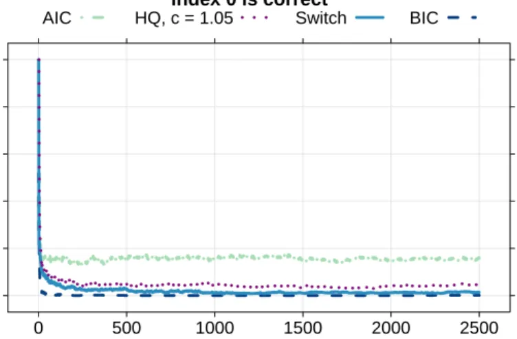
is true. N = 1000 data sets of length n = 2500 are generated from a standard normal distribution, and AIC, BIC, HQ withc = 1.05 andδsw are evaluated at each sample size.
The average selected model index (0 forM1, 1 forM2) is given in Figure1.
In the second setting,M2 is true. The data is generated from a normal distribution with
mean 0 and a variance that is varied. For each value of σ, N = 1000 datasets of length
n= 2500are generated, and the four model selection criteria are evaluated at that sample size. The average selected model index is given in Figure2.
The results are as expected. When the complex model is true, AIC is most likely to select it, at the cost of inconsistency when the simple model is true. BIC is the slowest to correctly select the complex model and the first to correctly select the simple model. HQ and δsw
show intermediate behaviour, HQ being slightly more likely to select the complex model. To illustrate strong consistency and optional stopping, three scenarios are considered: 1. M0 vs M1, data from a standard normal distribution (“scenario 1" — Theorem
2/Corollary 1 implies that switching defines a test that is robust with respect to optional stopping).
2. M1 vs M2, data from a standard normal distribution (“scenario 2”, Theorem 2 does
not only imply robustness, because null model is composite).
3. M1 vs M2, data from a normal distribution with mean 35 and variance 1 (“scenario
3", Theorem 2again does not imply robustness).
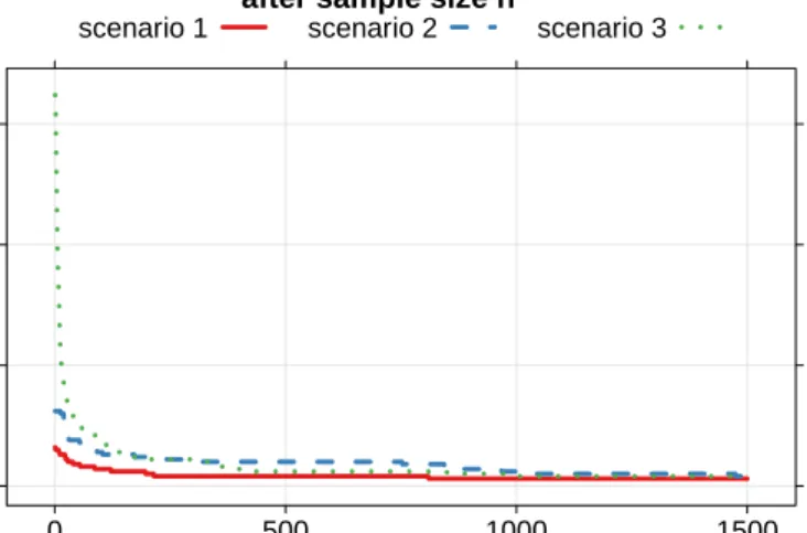
We create N = 1000 data sets of length nmax = 10000 in each scenario. We select the
complex model when δsw is larger than 20 (in terms of the robust p-value interpretation of
Theorem 2, this corresponds to a significance level of 0.05). We estimate two probabilities at each sample sizen:
• The probability that there will ever be a model index after nat which the complex model will be selected (Figure 3), approximated by checking whether the complex model is selected at any sample size betweennand3nmax.
• The probability that there exists a model index beforenat which the complex model would have been selected (Figure4).
Figure3 can be interpreted as a check whether strong consistency holds — if it does, then the probabilities should converge to0as n→ ∞. Van Erven et al.’s (2007) theorem implies that strong consistency holds in all three scenarios, and the graphs confirm this — even though for scenario 3, in which data comes from aµ∈M0that is ‘atypical’ under the prior,
it takes a bit longer — illustrating that strong consistency is not a uniform notion. The graph also illustrates that strong consistency can be viewed as an asymptotic, nonuniform version of robustness to optional stopping — it implies that from some sample size (which may be very large though) onwards, one will never again falsely reject no matter how long one keeps sampling.
Figure 4 refers to nonasymptotic optional stopping: in scenario 1, the conditions from Theorem 2hold, and indeed the figure shows that the probability that the complex model is ever incorrectly selected even when optional stopping is used, is bounded by 0.05 (the observed bound is 0.015). In scenarios 2 and 3, the conditions from Theorem2do not hold. In scenario 2, the behaviour of the switch criterion is similar to scenario 1. However, in scenario 3, the probability of a false rejection opportunity before sample size n is not bounded by 0.05, but quickly goes to 0.15. We clearly see thatδsw is not robust to optional stopping in
scenario 3.
When the simplest model is not a singleton, the choice of prior on the model parameters (in scenarios 2 and 3 onµin M1 and on(µ, σ2)inM2) affects the results. In both scenario
2 and 3, δsw must still satisfy the weak, prior-expected version of robustness (5.3), as we
have seen in Section 5.3. In scenario 2, the prior is centered at the data-generating value of zero and we do observe actual robustness. In scenario 3 however, the prior is centered at zero while the data is generated with a mean of 35, 3.5 standard deviations away from the prior mean — thusµis ‘atypical’ under the prior, and, as the figure shows, nonasymptotic robustness is violated.
6. Discussion and Future Work
In this paper we showed that switching combines near-rate optimality, consistency and, for singleton M0, robustness to optional stopping. We end the paper by highlighting three
issues which, we feel, need additional discussion: first, the desirability of consistency; second, whether there is anything ‘special’ to the switch criterion as opposed to other possible trade-offs between risk optimality and consistency; and third, the limitations of switching in its current form.
Consistency Since the desirability of consistency, in the sense of finding the smallest model containing the true distribution, is somewhat controversial, let us discuss it a bit further. The main argument against consistency is made by those adhering to Box’s maxim ‘Essentially, all models are wrong, but some are useful’ (Box and Draper,1987). According to some, the goal of model selection should therefore not be to select a non-existing ‘true’ model, but to obtain the best predictive inference or best inference about a parameter
Average selected model index Index 0 is correct n 0.0 0.2 0.4 0.6 0.8 1.0 0 500 1000 1500 2000 2500
AIC HQ, c = 1.05 Switch BIC
Fig 1.N = 1000data sets of lengthn= 2500are generated from a standard normal distribution and the
criteria are evaluated at each sample size. The figure shows the average selected model index (0 forM1, 1
forM2). The true index is 0.
Average selected model index Index 1 is correct σ 0.0 0.2 0.4 0.6 0.8 1.0 1.00 1.05 1.10
AIC HQ, c = 1.05 Switch BIC
Fig 2.N = 1000data sets of lengthn= 2500are generated from a normal distribution with mean 0 and
varianceσ2for a range of values ofσ. The criteria are evaluated atn= 2500. The figure shows the average
Probability of false rejection opportunity after sample size n
n 0.00 0.05 0.10 0.15 0 500 1000 1500
scenario 1 scenario 2 scenario 3
Fig 3. N= 1000data sets of lengthnmax= 10000in each scenario, from the simple model. The complex
model is selected whenδsw(xn)>20. Estimated probability that there exists a model index afternat which
the complex model will be selected. Results shown up to n= 1500for clarity. Aftern= 1500, the three curves are indistinguishable and all very close to zero.
Probability of false rejection opportunity before sample size n
n 0.00 0.05 0.10 0.15 0 2000 4000 6000 8000 10000
scenario 1 scenario 2 scenario 3
Fig 4. Setting as Figure3. Estimated probability that there exists a model index before nat which the
(Burnham and Anderson,2004; Forster,2000). Another issue with consistency is that it is a ‘nonuniform’ notion, which in our context means that — as is indeed easy to see — it is impossible to give a bound on the probability under Pµ of selecting the wrong model at
sample sizenthat converges to0uniformly for allµ∈M. This nonuniformity implies that consistency is of little practical consequence for post-model selection inference (Leeb and Pötscher,2005).
As to the first argument, one can reply that there do exist situations in which a model can be correct, for example in the field of extrasensory perception (Bem, 2011), in which it seems exceedingly likely that the null model (expressing that no such thing exists) is correct; another example is genetic linkage (Gusella et al., 1983; Tsui et al., 1985). The second argument is more convincing, but only to argue that even if consistency holds, a method may not be very useful in practice. It does not contradict that consistency can sometimes be a highly desirable (but never the only highly desirable) property — we feel that this is the case whenever we are not purely interested in prediction but instead are also seeking to find out whether a certain structural relationship (e.g. dependence between variables) holds or not.
Going one step further, it seems a good idea to study model selection methods not in terms of the asymptotic, nonuniform notion of consistency but instead by a more tangible finite-sample analogue. For the case of just two models, Type-I and Type-II errors provide exactly this analogue — note that if both errors go to 0 asn→ ∞, this implies consistency. Thus, thepracticalimportance of the present work, for us, is mostly that model comparison by switching defines, like Bayes, a robust null hypothesis test — providing Type-I errors irrespective of the stopping rule and thus more in line with actual practice — yet has better Type-II error behaviour, allowing the Type-II error to become small (i.e. the power to go to 1) whenever the true distribution sits at a distance of order p(log logn)/n rather than
p
(logn)/n, as with Bayes. We only showed robustness for singletonM0, however, and our
simulations show that it may fail for composite M0, so the major goal for future work is
therefore, to come up with methods that are robust to optional stopping also under composite M0.
How special is the switch distribution? Since Yang proved that in general, the conflict between consistency and risk-optimality is not resolvable, one might argue that any model selection rule just picks some position in the spectrum of behaviours of consistency vs. risk-optimality. For example, one might have a modified HQ criterion which picks M1
if, using the same setup and notation as in (5.4),
n X i=1 ˜ Xi ≥p
nlog log logn. (6.1)
By the central limit theorem, such a method will be consistent, yet when combined with an efficient estimator will achieve the minimax estimation rate up to alog log lognfactor, improving on the switch criterion by an additional logarithm. Note however that both the switch distribution and HQ (withc >1) achievestrong consistency. The meaning of strong consistency is illustrated in Figure3above: it means that, from somenonward, the wrong model will never be selected any more, no matter how long one keeps sampling. It is easy to see from the law of the iterated logarithm that any strongly consistent method can have rate no faster than order (log logn)/n — in particular, (6.1) is not strongly consistent. Thus, in this sense both switching and HQ do take a special place in the consistency vs. risk-optimality spectrum as obtaining the fastest rates compatible with strong consistency, which may be viewed as asymptotic robustness to optional stopping. While this may mostly be of theoretical interest, the switch distribution also takes a special place in terms of its nonasymptotic robustness to optional stopping: again, the law of the iterated logarithm implies that any model comparison method that defines a robust hypothesis test cannot achieve estimation rate better than order(log logn)/n. Again, the main open question here is whether one can modify it so that robustness for compositeM0 is achieved as well.
Future Work — Limitations of the Switch Distribution and Our Results Whereas the results in this paper all apply to the original switch distribution as defined by Van Er-ven et al. (2007) and a simplification thereof, for full robustness to optional stopping with composite M0, some substantial changes have to be made, as suggested by the results in
Figure4. Initial research suggests that such a modification of the switch distribution might indeed be constructed, based on techniques inRamdas and Balsubramani (2015); whereas, compared to Bayes factor testing, in the current switch criterion,pB,1is modified to another
distribution andpB,0can remain the same, in this new version we would also have to change
pB,0— the resulting distribution would not have a Bayesian interpretation any more. While
this work is still under development, to avoid the nonrobustness seen in Figure4as much as possible, for the time being we recommend using flat priors (but in this case, not completely flat - Jeffreys’ prior onµis improper, in which case Theorem2holds in none of the scenarios and simulations — not reported here — show that optional stopping robustness is violated). Another limitation lies not in the switch distribution, but in our results: these are re-stricted to two nested exponential family models. It would be interesting to extend them to more than two models — highlighting the distinction between model selection and test-ing — and gotest-ing beyond exponential families. We are hopeful that switchtest-ing still behaves well in such contexts — we note that the risk rate convergence results of Van Erven et al. (2012) were for countable, possibly infinite collections of completely general models — but they invariably dealt with the cumulative risk. While all our experiments suggest that small cumulative risk usually goes together with small instantaneous risk, formal analysis of the switch criterion’s instantaneous risk is far more difficult, and the present paper heavily relies on sufficiency to do so — so extension of our results beyond exponential families would be difficult.
Before doing so, we would prefer to modify the switch distribution further, since the present version has a drawback when used in nonsequential settings: the precise results it gives are dependent on the order of the data, even if all the models under consideration are i.i.d. Thus, it would be interesting and challenging to design an alternative, order-independent method that, like the switch distribution, is strongly consistent, near rate-and power-optimal, rate-and is robust to optional stopping under compositeM0. Such a method
would essentially truly achieve the best of the three worlds we considered in this paper — and this is the method we aim for in our future research.
Acknowledgements
The central result of this paper, Theorem 1, already appeared in the Master’s Thesis (Van der Pas,2013) for the (very) special case wherem1= 1andm0= 0, but the proof supplied
there contained a (serious but repairable) error. We are grateful to Tim van Erven for pointing this out to us. We are also thankful to the anonymous referees and to Hannes Leeb for raising the issue of whether the switch distribution has a ‘special’ place on the spectrum of a model selection criterion’s possible risk and consistency behaviors.
We start by listing some well-known properties of exponential families which we will repeatedly use in the proofs. Then, in SectionD, we provide a sequence of technical lemmata that lead up to the proof of our main result, Theorem1. Finally, in SectionE, we compare the switch distribution and criterion as defined here to the original switch distribution and criterion of Van Erven et al. (2012).
Additional Notation Our results will often involve displays involving several constants. The following abbreviation proves useful: when we write ‘for positive constants~c, we have ...’, we mean that there exist some (c1, . . . , cN) ∈ RN, with c1, . . . , cN > 0, such that ...
holds; hereN is left unspecified but it will always be clear from the application what N is. Further, for positive constants~b= (b1, b2, b3), we define small~b(n)as
small~b(n) = (
1 ifn < b1
and we frequently use the following fact. Suppose thatE1,E2, . . .is a sequence of events such
thatP(En)≤small~b(n). Then we also have, for any eventA, and for alln,
P(A,Enc)≥P(A)−small~b(n), (.2)
as is immediate fromP(A,Enc) =P(A)−P(A,En)≥P(A)−P(En).
The components of a vector µ∈ Rn are given by (µ1, µ2, . . . , µn). If the vector already
has an index, we add a comma, for exampleµ1= (µ1,1, µ1,2, . . . , µ1,n). A sequence of vectors
is denoted byµ(1), µ(2), . . ..
Appendix A: Definitions Concerning and Properties of Exponential Families
The following definitions and properties can all be found in the standard reference ( Barndorff-Nielsen,1978) and, less formally, in (Grünwald,2007, Chapters 18 and 19).
A k-dimensional exponential family is a set of distributions on X, which we invariably represent by the corresponding set of densities {pθ|θ∈Θ}, whereΘ⊂Rk, such that any
memberpθ can be written as pθ(x) =
1
z(θ)e θTφ(x)
r(x) =eθTφ(x)−ψ(θ)r(x), (A.1) where φ(x) = (φ1(x), . . . , φk(x))is a sufficient statistic, ris a non-negative function called
thecarrier,zthepartition functionandψ(θ) = logz(θ). We assume the representation (A) to beminimal, meaning that the components ofφ(x)are linearly independent.
The parameterization in (A.1) is referred to as thecanonical ornatural parameterization; we only consider families for which the setΘis open and connected. Every exponential family can alternatively be parameterized in terms of itsmean-value parameterization, where the family is parameterized by the meanµ=Eθ[φ(X)], with µtaking values inM ⊂R, where
µas a function ofθis smooth and strictly increasing; as a consequence, the setM of mean-value parameters corresponding to an open and connected set Θ is itself also open and connected. Whenever for data x1, . . . , xn, we have 1n
Pn
i=1φ(xi)∈M, then the maximum
likelihood is uniquely achieved by theµthat is itself equal to this value,
b µ(xn) = 1 n n X i=1 φ(xi). (A.2)
We thus define the maximum likelihood estimator (MLE) to be equal to (A.2) whenever
1 n n X i=1 φ(Xi)∈M. (A.3)
Since the result below which directly involves the MLE (Lemma 3) does not depend on its value for xn with 1
n Pn
i=1φ(xi) 6∈ M, we can leave µb(x
n) undefined for such values.
However, if we want to use the MLE as a ‘sufficiently efficient’ estimator as used in the statement of Theorem 1, we need to define µb(xn) for such values in such a way that the
‘sufficiently efficient property’ (4.1) is satisfied. The following examples show various ways of constructing such sufficiently efficient estimators.
Example 3. [Sufficient Efficiency for MLE’s for squared (standardized) error and Hellinger] For many full families such as the full (multivariate) Gaussians, Gamma and many others, (A.3) holds µ-almost surely for each n, for all µ ∈ M. If we compare two familiesM0 andM1 given in their mean-value parameterization withM0⊂M1 whereM1
is any such family, then the MLE is almost surely well-defined for M1 and thus we need
not worry about the issue indicated above. We can then take µ˘1 :=bµ1 to be the MLE for
M1. To get a sufficiently efficient estimator forM0, we takeµ˘0 to be the projection ofbµ1
on the first m0 coordinates (usually (A.3) will still hold for M0 and then thisµ˘0 will also