A Hyper-Heuristic Ensemble Method for Static
Job-shop Scheduling
Emma Hart
[email protected]Institute for Informatics and Digital Innovation, Edinburgh Napier University, Edinburgh, EH10, UK
Kevin Sim
[email protected]Institute for Informatics and Digital Innovation, Edinburgh Napier University, Edin-burgh, EH10, UK
Abstract
We describe a new hyper-heuristic methodNELLI-GPfor solving job-shop schedul-ing problems (JSSP) that evolves an ensemble of heuristics. The ensemble adopts a divide-and-conquer approach in which each heuristic solves a unique subset of the in-stance set considered. NELLI-GPextends an existing ensemble method called NELLI by introducing a novel heuristic generator that evolves heuristics composed of linear sequences of dispatching rules: each rule is represented using a tree structure and is itself evolved. Following a training period, the ensemble is shown to outperform both existing dispatching rules and a standard genetic programming algorithm on a large set of new test instances. In addition, it obtains superior results on a set of 210 benchmark problems from the literature when compared to two state-of-the-art hyper-heuristic approaches. Further analysis of the relationship between hyper-heuristics in the evolved ensemble and the instances each solves provides new insights into features that might describe similar instances.
Keywords
Job-shop-scheduling, dispatching rule, heuristic ensemble, hyper-heuristic, genetic programming
1
Introduction
The Job Shop Scheduling problem (JSSP) is one of the most researched combinatorial problems studied by practitioners over recent decades, due to its relevance in many industrial applications. The simplest form is known as thestatic JSSP: a number of operations that need to be scheduled across multiple machines, with all operations available at the start. Dispatching rules that derive a priority index for each operation to be scheduled provide a quick and simple method for creating a schedule (Baker, 1984), and hence for practical reasons are commonly used in real-world applications. Many dispatching rules are described in the literature, designed by hand by human-experts, although according to Geiger et al. (2006), often through considerable effort. In an effort to automate this, hyper-heuristic methods have been used to create novel, reusable dispatching rules. A comprehensive recent survey is provided by Branke et al.
(2015) who summarize the state-of-the-art, noting that the most common approach has been to use variable-length grammar-based methods (e.g. genetic programming) to generate new dispatching rules. While this has achieved much success, they highlight a number of open questions and challenges, the first of which is the need to deal with complex scenarios by evolvingensemblesof heuristics, rather than a single rule.
Currently, a few examples of small ensembles that evolvepairsof heuristics exist, e.g. (Miyashita, 2000; Nguyen et al., 2014a; Park et al., 2013). Most recently, Park et al. (2015) evolve a larger ensemble of rules in which each heuristic in the ensemble votes to determine the priority of an operation at each iteration, using a similar methodology to ensemble approaches to classification typically seen in machine learning (Valentini and Masulli, 2002). From an optimisation perspective, Smith-Miles et al. (2014) point out that any given algorithm will have individual weaknesses on a given set of instances. Ensemble methods in which a mixture of algorithms is used to solve a set of instances would therefore appear a fruitful line of research. We propose an ensemble approach in which a set of heuristics is evolved using GP, each of which generates a complete solution to a subset of instances in a distinct region of the instance space (i.e. the set of problem instances of interest). This can be be loosely described as ‘mixture-of-experts’ model to borrow terminology from the machine learning literature. It is also similar to thealgorithm portfoliomethods that are common in Operations Research, particularly for solving SAT problems, e.g. (Leyton-Brown et al., 2003). However, in contrast to many portfolio methods that focus mainly on selection from a portfolio, our approach addresses portfolio composition, ensuring that the portfolio contains a behaviourally diverse range of algorithms.
Our approach extends a previously described ensemble method called NELLI, that has been extensively tested in the bin-packing domain (Sim et al., 2015) and on a small set of 62 JSSP instances (Sim and Hart, 2014). NELLI-GP extends NELLI by evolving a pool of novel dispatching rules, each represented as an expression tree. The novel rules are combined into variable length sequences called heuristics, which are themselves subject to evolution. Using a large set of static JSSP instances, we address two main questions using NELLI-GP:
• Do evolvedheuristics, composed of variable lengthsequencesof evolved dispatch-ing rules, outperform the individual evolved rules?
• Doensemblesof evolved heuristics outperform individual heuristics?
Our approach extends existing work on tree-based rule evolution of single dispatching-rules by considering an extended node set and multiple methods for se-lection of eligible jobs. It extends current approaches toensemblemethods in that the role of each member of the ensemble is to solve a subset ofinstances, rather than vot-ing to prioritise individualoperations. Evaluation on over 700 problem instances shows significant improvement with respect to existing dispatching rules, and to state-of-the approaches (Park et al., 2015; Nguyen et al., 2013b), improving on published results on benchmark sets by up to 16%. Finally, analysis of the ensemble in terms of map-ping heuristics to instances provides new insights into the relationship between simple instance parameters and algorithmic performance.
The paper proceeds with a brief introduction to JSSP and to previous approaches for automating the production of dispatching rules. In section 4 we provide both a
conceptual and algorithmic description of the approach, clarifying the modifications that were made to NELLI and describing the new problem generator. After providing detailed experimental results, the paper concludes with an analysis section that pro-vides some insight into the function of the individual elements of the ensembles, the diversity of heuristics, and the difficulty of the problems in the instance space.
2
Background
Using theα|β|γnotation (Graham et al., 1979) the two JSSP problems investigated are denoted asJ m||CmaxandJ m||PωiTiwhere the termJmtranslates as a Job Shop
envi-ronment and the last term corresponds to the objective (Makespan (Cmax) and Summed
Weighted Tardiness (SWT) respectively). An nxmJSSP problem has a set of njobs,
{Ji}1≤j≤n andmmachines, {Mk}1≤k≤m. Each job Ji containsmoperations, each of
which has processing timepjkand weight given bywi. Every job is processed on every
machine with no recursion allowed. Each job has a release timeriwhich imposes a hard
constraint on the earliest start time of a job and a due time ofdi which imposes a soft
constraint on the time that the job should be completed by. Machines process a single operation at a time and all machines are available for the duration of the schedule.
2.1 Dispatching Rules
Many simple dispatching rules have been developed to quickly prioritise operations in order to select an appropriate operation for scheduling in an iterative process (see Panwalkar and Iskander (1977); Haupt (1989); Blackstone et al. (1982)). Typically, rules are hand-designed by experts in a trial and error-process (Geiger et al., 2006), and each one optimises one or a limited number of scheduling objectives based on some partic-ular conditions. CompositeDRs combines single dispatching rules into a new rule and have been shown to outperform single DRs (Nguyen et al., 2013a). Both types of DR typically fall into one of two categories: DRs that can be evaluated before a schedule is commenced (e.g. Job Arrival Date and Operation Processing Time) or DRs that return different priorities for operations as the schedule is built (e.g. Number of Remaining Operations).
Many simple dispatching rules have been known for decades — a comprehensive survey in Panwalkar and Iskander (1977) describes over one hundred. Some of the earliest hyper-heuristic approaches to scheduling (though the term was not in use at the time) recognised improved performance could be achieved by combining existing dispatching rules into sequences that could be applied iteratively to build a solution. For instance, Ulrich and Erwin (1995) and Hart and Ross (1998) both use evolutionary algorithms to search for promising sequences of dispatching rules, showing promising results compared to the single rules.
In addition to specifying priority, a dispatching rule needs to also specify the el-igible job set, i.e., the subset of jobs that should be prioritised by the rule. Non-delay selection only considers jobs that are currently waiting to be scheduled, and hence min-imises idle-time. In the majority of hyper-heuristics that generate dispatching rules, el-igibility is limited to waiting jobs, i.e. follows the non-delay method. Non-delay sched-ules are not guaranteed to be optimal; the Giffler-Thompson algorithm (Giffler and Thompson, 1960) includes in the list of eligible jobs those arriving in the near future, before the shortest operation of waiting jobs can be completed. Hyper-heuristic
meth-ods that adopt this approach (or variants of it) include (Geiger et al., 2006; Miyashita, 2000; Pickardt et al., 2013). Rather than pre-defining eligibility, the hyper-heuristic it-self can optimise the method by which eligible jobs are selected. Hart and Ross (1998) evolved an extra parameter for each rule that defined the method that should be used to generate the conflict set of operations; Nguyen et al. (2013a) propose a representation for evolving scheduling rules that incorporates a hybrid scheduling strategy between non-delay and active scheduling. InNguyen et al. (2013b), a separate function for the non-delay factor is evolved which can then adapt to changing shop conditions.
2.2 Evolving Novel Dispatching Rules
Despite the large number of existing dispatching rules and proposed methods for com-bining them, interactions between scheduling rules can be complex; in order to address this, more recent research has attempted to automate the process of designing rules, through the use of Genetic Programming to evolve arithmetic expressions of rules. This is ahyper-heuristicapproach in that the space of heuristics (dispatching rules) is searched, rather than the space of potential solutions (schedules). A very comprehen-sive survey of hyper-heuristic approaches to automated design of dispatching rules is provided in (Branke et al., 2015).
Most hyper-heuristic methods evolve a single dispatching rule. For example, Tay and Ho (2008) successfully evolved rules that determined the priority of operations to be scheduled for static problems. This work was later shown to be less useful in dynamic cases. Hildebrandt et al. (2010) advanced this work by using four varied training scenarios and found effective but complex rules. Noting that most rule-based approaches lack a global-perspective in that they only consider the current state of a machine and its queue.
Nguyen et al. (2013b) evolve iterated dispatching rules that iteratively improve the schedules by utilising the information from completed schedules; in (Nguyen et al., 2013a), they extend the terminal set available to GP to include both recorded infor-mation regarding a previous schedule,‘look-ahead’ inforinfor-mation and composite DRs, finding good results on static JSSP problems. Hunt et al. (2014) extend this approach of using ‘less-myopic’ information, evolving new rules with an extended terminal set that were tested on a set of randomly created test scenarios. Their results show evolution of better DRs in terms of total weighted tardiness across the test simulation scenarios with high utilisation. In relation to dynamic JSSP problems, Nguyen et al. (2014b) compare surrogate-assisted selection methods in conjunction with GP, and automatic program-ming via iterated local search in (Nguyen et al., 2015). Note that in addition to trees, other representations of dispatching-rules are possible, for example using neural net-works to represent a function or simple linear combinations of attributes. However a recent paper by Branke et al. (2014) evaluated potential representations and concluded that in terms of solution quality then the expression tree representation was preferable. The GP systems described above evolve asinglerule that should generalise across a range of benchmarks. Another strand of research utilises GP to evolve multiple rules that are used collaboratively to solve problems. Miyashita (2000) develop a system called GP-3 that evolves two dispatching rules and a choice function that selects be-tween the two rules depending on whether a machine creates a bottleneck; this shows improvement over the use of a single evolved rule. Nguyen et al. (2014a) consider two approaches to evolving rules for dynamic JSSPs. In the first approach, a single
individ-ual is evolved that contains two separate subtrees that together specify a scheduling policy. In their second approach, a cooperative co-evolution method inspired by Potter and De Jong (2000) is used to evolve trees in two separate sub-populations: trees from each sub-population are combined to specify a complete policy, and three objectives are used to select individuals based on dominance criteria.
2.3 Collectives of Rules
GP has previously been used to evolve ensembles of rules in the classification domain, e.g. (Downey et al., 2012; Bhowan et al., 2013, 2014). The evolved ensembles pro-mote behavioural diversity amongst the evolved classifiers, and have proved promis-ing when applied to classifypromis-ing unbalanced data-sets. Each evolved classifier votes on the class of a given data-record, with the majority vote recorded. In the hyper-heuristic JSSP domain, at the time of writing we are aware of only one ensemble ap-proach. Park et al. (2015) extend the cooperative co-evolution method first proposed by Nguyen et al. (2014a) to evolvessub-populations of trees; a set consisting of one tree from each sub-population is formed and each member of the subset votes as to which operation should be selected for scheduling. The operation with the most votes is then scheduled. The approach shows promising results but was limited to testing on 80 problems.
In contrast to the above ensemble method in which members of the ensembleeach votes as to which operation should be scheduled, we have previously described a sys-tem called NELLI that evolves an ensemble in which each member of the ensemble ‘wins’ a unique subset of the instances under consideration (Sim et al., 2015, 2013; Sim and Hart, 2014). NELLI uses a method inspired by Artificial Immune Systems (AIS) to evolve a set of heuristics, which are behaviourally diverse in the sense that each solves different subsets of a large instance set. This approach bears considerable re-semblance tobagging (bootstrap aggregating) approaches from the machine learning literature (Breiman (1996)) which have been shown to improve the stability and accu-racy of machine learning algorithms, by reducing variance and avoiding overfitting. The approach can also be considered asmixture of expertsmethods (Valentini and Ma-sulli (2002)): in these methods a supervising learner divides the input space and assigns an appropriate element of the ensemble to each division. WhileNELLI-GPretains the core AIS element of NELLI which ensures diverse heuristics are retained, it replaces the component that evolves the heuristics, using GP to evolve new dispatching rules which are sequenced into new heuristics.
3
Method
In NELLI-GP, an ensembleEis defined by a tuplehH, R, Di.H specifies the maximum number ofheuristicsin the ensemble, each of which is composed of a sequence ofrules. The maximum length of the rule sequence is denoted byR. Each rule is defined by a tree that can have maximum depthD. Thus, an ensemble signified by the expres-sionH5−R3−D10for example describes an ensemble composed of a maximum of 5 heuristics, each of which is composed of a sequence of rules of maximum length 3, and where each rule has maximum depth 10. The creation of trees, rules, and heuristics that forms a key contribution of this paper are described in turn below.
3.1 Tree-based Dispatching Rules
In contrast to previous work in which NELLI used dispatching rules taken directly from the literature (Sim and Hart, 2014), in NELLI-GP we formulate novel dispatching rules as trees of depthd, where0 ≤ d≤ dmax. The tree returns a real value for each
operation that can be considered for scheduling — these values are subsequently used to prioritise each operation. Trees are formulated using a set of terminal and function nodes described below.
3.1.1 Terminals & Function Nodes
We use a large set of function nodes as defined in table 2. The terminal node set contains 28 dispatching rules, compared to 14 in Hunt et al. (2014) and 7 in Tay and Ho (2008). The majority of these have been obtained from the literature and includes examples of both simple and composite dispatching rules and examples from each of the three classes defined in section 2.1 —static, dynamic, less-myopic. Additional terminals have been added to increase diversity.
Note that many of the acronyms used here differ from those commonly used in the literature due to the fact that the set of priorities returned by a rule can be or-dered eitherascending or descending. For example the Shortest Processing Time rule (SPT) named OpPT here can sort operations from smallest to largest or from largest to smallest, depending on whether the terminal is set as positive or negative. Terminals prefixed with Op, J, or M denote that they operate on the operation, its associated job or its allocated machine. For example for each operation to be prioritised, MTPT returns the total processing time of the operations to be scheduled on the associated machine and JTPT returns the total processing time of the job.
The list includes simple DRs such as Weighted Shortest Processing Time (WSPT), Earliest Due Date (EDD) and Minimum Slack (MS) (named JWPT, JDD and JS respec-tively). These DRs have been shown to provide optimal solutions for the 1||Pω
jTj
single machine problem when release dates and due dates are zero (WSPT), or when they are sufficiently spread out (EDD or MS). The terminal set also includes composite DRs from the literature such as Apparent Tardiness Cost (JATC) which encapsulates features of both WSPT and MS. JATC has been shown to outperform its component parts in Vepsalainen and Morton (1987) for the SWT objective. Some less myopic rules such as Next Operation Processing Time (OpNPT) are also implemented.
When a terminal node is added to a tree, it is randomly assigned as apositive or negativenode, i.e. a rule can order its list of operations from largest to smallest or vice-versa. Thus in effect, the size of the terminal set is doubled.
3.1.2 Rule Wrappers: Eligible Operations
Each newly generated tree is encapsulated in a wrapper named a rule. A rule is ran-domly assigned a labelA, B, Cspecifying the algorithm that should be used to generate the setS∗ of operations that are eligible for scheduling, thus expanding the search-space of possible rules. Algorithm A is a modified version of the Giffler and Thompson algorithm (Giffler and Thompson, 1960) described in Algorithm 1; Algorithm B is the Non-Delay algorithm (Baker, 1984) described in Algorithm 2; Algorithm C is the set of all available waiting operations.
Table 1: Terminals: Dispatching Rules Terminal Nodes
Acronym Description JAPT Average Job Processing Time JATC Job Apparent Tardiness Costvar= 0.35 JDD Job Due Date
JEγD From Arkin 1991γ= 1
JPTSF Job Processing Time So Far JRPTI Job Remaining Processing Time
(including this op)
JRPT Job Remaining Processing Time (NOT including this op) JS Job Slack Time JTPT Job Total Processing Time JWPT Job Weighted Processing Time JW Job Weight
JAD Job Arrival Date MIT machine idle time (so far) MLFT Machine Last Op Finish Time MPTRI Machine Processing Time Remaining
(inclusive of the operation)
Terminal Nodes
Mnemonic Description
MPTR Machine Processing Time Remaining (not including the operation) MPTSF Machine Processing Time So Far
(not including idle)
MTPT Machine Total Processing Time (sum of all operations to be scheduled) OpEST Operation Earliest Schedule Time OpFCFS Operation First Come First served OpNPT Next operation in the job’s processing time
(or 0 if last op in job)
OpNRO Number of Remaining Operations OpPPT Previous operation from the job’s processing
time (or 0 if first op in job) OpPT Operation Processing Time OpWPT Weighted Processing Time OpRT Random Operation INT Random Integer Value REAL Random double between 0 and 1
Table 2: Function Nodes Function Set
Mnemonic #Ops Returns
ABS 1 Absolute Value of Op + 2 Sum of Op 1 and Op 2
- 2 Difference between Op 1 and Op 2 X 2 Product of Op 1 and Op 2
/ 2 Protected Division of Op 1 by Op 2∗ NEG 1 Negation of Op 1
IGTZ 3 If Op 1≥= 0; Op 2 else Op 3 Exp 1 The Exponential of Op 1
MAX 2 The maximum value of Op 1 and Op 2 Comp 2 If Op 1<Op 2 returns -1
If Equal returns 0: Else returns 1
∗
IfOp2 = 0,∞is returned
Algorithm 1Giffler & Thomson
1:Calculate the set C of all operations that can be scheduled next
2:Calculate the completion time of all operations in C, and let m* equal the machine(s) on which the minimum completion time t is achieved.
3:LetS∗denote the conflict set of operations on machine(s) m* - this is the set of operations in C which take place on m*, and whose start time is less than t.
Algorithm 2Non Delay
1:Calculate the set C of all operations that can be scheduled next
2:Calculate the starting time of each operation in C and letS∗equal the subset of operations that can start earliest
MPTRI
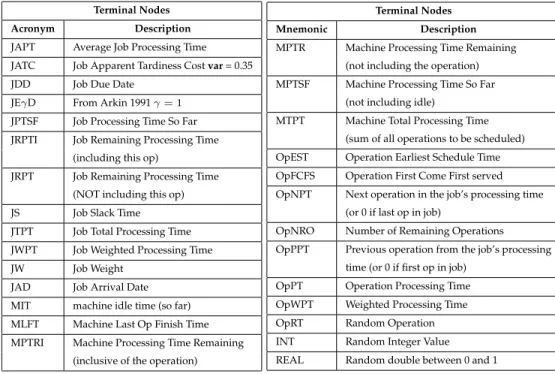
Conflict Set Dispatching Rule (D=0) (a) Max X-JAD -JRPTI MTPT MIT
B Conflict Set Dispatching Rule (D=2) (b)
Figure 1: Example rules comprising a conflict set and a tree dispatching rule of depth 0 (left) and 2 (right). Terminal nodes prefixed with-return a negated value
The first two algorithms are known to generate schedules from a reduced solu-tion space that includes the optimal solusolu-tion. The Giffler and Thompson algorithm is modified as shown in algorithm 1 such that if more than one machine shares the same minimum completion time, then all machines with that time are included inS∗. The third method is included given that hyper-heuristics are often used in situations in which optimality is not required, merely an acceptable solution found quickly — note however, that the evolutionary process might subsequently discard this rule. An oper-ation is chosen for scheduling fromS∗according to the value returned by the priority rule.
Note that there are28∗2∗3 = 168possible dispatching rules described by trees of depth = 0 only: a rule can contain one of 28 terminals, each of which can be set as positive or negative and use one of the 3 possible conflict sets. The number of potential complex rules composed of trees of depth>0is obviously considerably larger.
3.2 Heuristics
A heuristic,hi, is defined as a variable length sequence of rules, of minimum length 1
and maximum lengthR. To produce a solution for a problem instance, each rule in the heuristic is applied in turn and schedules a single operation. After the last rule in the sequence is used the procedure repeats starting from the first rule until all operations have been scheduled. When a rule is selected, the subsetS∗ of operations to be con-sidered for scheduling is generated according to the scheduling rule A,B,C defined by the rule. The tree defined by the rule is then applied to sort the available operations. The first operation from the sorted list is then selected. If more than one operation may be placed at the head of the sorted list (i.e. set of equal values is returned) then one is selected randomly. The selected operation is scheduled at the earliest available time on its predetermined machine as determined by the maximum of the completion time
of the last operation to be processed on the machine, the completion time of the last operation from the selected operations associated job and the job’s arrival time.
3.3 Evolving Ensembles of Heuristics
Evolution of the ensemble is managed using the NELLI method previously mentioned in section 2, modified in order to cope with the use of tree-based rules. In brief, the algorithm provides a cooperative method of evolving a set of heuristics that interact to cover a problem space, favouringheuristicsthat are able to find a niche in solving at least one problem better than any other heuristic in the system. Heuristics are sustained in the system by ‘winning’ instances, e.g. achieving a result on an instance that is better than anything else in the ensemble.
The heuristics in the ensemble continuously adapt due to evolutionary processes that continually trial new heuristics, and the size of the ensemble is an emergent prop-erty of the system. On the one hand, this enables the network to both continually improve its responseand adapt to changing problem instances. On the other, it pro-vides an immediate solution to new problem instances that appear as each heuristics generalises over some part of the problem space. A full description of the algorithm can be found in Sim et al. (2013, 2015); Sim and Hart (2014); Hart and Sim (2014) which describes applications in which heuristics were formed from pre-defined rules only.
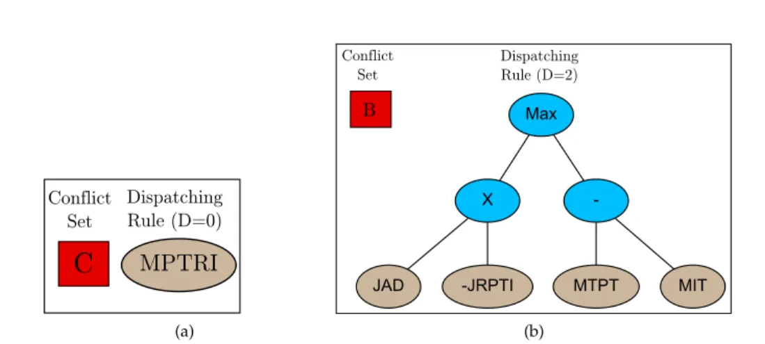
4
Implementation
A conceptual view of the system is given in figure 2 and is described by Algorithm 3. The system contains three key components: a continual stream of problem instances (theproblem-space), a continual stream of novel heuristics and a network of heuristics inspired by the idiotypic model of the immune system. The dynamics of the network determine the final constitution of the system in retaining only problems that are repre-sentative of characteristic regions of the problem space, and heuristics that solve prob-lems that cannot be solved by other heuristics. The system was originally proposed as a lifelong learningapproach that could autonomously adapt to changing problem charac-teristics (Sim et al., 2015) — here we use a modified form to evolve a fixed ensemble of heuristics that collectively map the problem space based on a training set of problems. As in any machine learning method, the quality of the system relies on the training set being representative of the problem space, hence a large, diverse set of problem instances is desirable.
The key improvements to previous work using NELLI Sim and Hart (2014) are provided by the new heuristic generator. Heuristics are now represented as sequences of novel tree-based dispatching rules. This also differs from previous work in Sim et al. (2015) that uses Single-Node genetic programming to represent bin-packing heuristics. The new approach provides increased diversity and results in a trained ensemble that better generalises across the problem space. A brief descripton of the core network is provided before describing the novel modifications in detail.
4.1 Immune Network
The immune network lying at the heart of the system is unchanged from the system used previously, e.g. (Hart and Sim, 2014), and is covered here briefly for clarity. The
Figure 2: NELLI-GP comprises three components: a heuristic generator to supply a continual stream of novel heuristics, a set of problem instances and a network inspired by the idiotypic network theory of the immune system. The heuristic generator is ex-panded (the shaded area) here by the addition of a Rule Generator
hstim= X p∈P δp ( δp = min (f(H0p))−f(hp) : if min (f(H0p))−f(hp)>0 δp = 0 : otherwise (1) pstim= X h∈H δh ( δh= min (f(H0p))−f(hp) : if min (f(H0p))−f(hp)>0 δh= 0 : otherwise (2) Where f(hp) is the result (MS or SWT) achieved by heuristic h on problem pand min (f(H0
p)) is the best result obtained on problem p by the rest of the ensemble H0=H −h
immune network models heuristics as antibodies and problems as pathogen. The ob-jective is to find a minimal repertoire of heuristics that effectively solve the problems being supplied to the system. A heuristic ‘wins’ a problem instance if it obtains a so-lution to the instance that is better thananyother heuristic in the system. The immune network promotesbehaviouraldiversity within the ensemble in that for a heuristic to persist it must win at least one problem. Similarly, a problem only survives in the system if it is won by onlyoneheuristic, i.e. it is representative of a hard part of the instance space. Both heuristics and problems have their behaviours governed by two variables — concentration and stimulation. The key steps of the immune network sim-ulation are described from line 10 onwards in Algorithm 3. Each iteration, after new problems and heuristics have been injected into the system, thestimulationlevels of both heuristics and problems are calculated using equations 1 and 2. Based on the stimulation received, concentration levels are adjusted up or down by a fixed amount
(∆c)depending on whether the stimulation value of a cell lies within upper and lower
Algorithm 3NELLI-GP Pseudo Code Require:H=∅ :The set of heuristics
Require:P=∅ :The set of problems currently in the system Require:E :The set of all available problems
1:repeat
2: p=U(0,1)
3: if(p≤probhm)∧(H 6=∅)then
4: Generate a newheuristichvia heuristic mutation1 5: else
6: Initialise a newheuristichvia heuristic initialisation2 7: end if
8: AddhtoHwith concentrationcinit
9: Addmax(np,|E − P|)randomly selected problem instances fromE − PtoPwith concentrationcinit
10: Calculatehstim∀h∈ Husing Equation 1
11: Calculatepstim∀p∈ Pusing Equation 2
12: Increment all concentrations (bothHandP) that have concentration< cmaxand stimulation>0by∆c
13: Decrement all concentrations (bothHandP) with stimulation≤0by∆c
14: Remove heuristics (fromH) and problems (fromP) with concentration≤0 15: while|H|>Hmaxdo
16: Remove the heuristic that contributes the least3to the ensemble 17: end while
18:untilstopping criteria met
For all experiments conducted hereprobhm= 0.9, np= 10, pm= 0.9
∆c= 50, cmax= 1000, cinit= 200
Hmaxis varied between 1 and infinity. Thestopping criteriais set to 10000 iterations
1 2are described by Algorithm 5 and Algorithm 4 respectively. 3
is determined as the heuristic that contributes the least to the global fitness achieved by greedily applying allh∈ Hto allp∈ P
of concentration(cinit)that allows them to persist in the network for a number of
iter-ations, even without receiving any stimulation. If any concentration level falls to zero or below it is removed from the system. Heuristics have an implicit affect on each oth-ers behaviour leading to complex network behaviour; for example a newly introduced heuristic that outperforms an existing heuristic may limit the stimulation received by the existing heuristic to such an extent that its concentration is reduced and it is even-tually removed from the network.
Note that there is noglobalfitness function: a new heuristic is only included in the ensemble if it wins at least one instance from another heuristic, hence every addition of a new heuristic necessarily improves global fitness. The stimulation level of a heuristic provides a measure of itsindividual fitness: this drives selection for mutation, providing evolutionary pressure for individuals to improve. Specialisation of heuristics to spe-cific niches with the instance space occurs due to the explicit need to win instances to survive.
4.2 Heuristic Generator
As previously described, a heuristic is composed of a sequence ofrules. Each rule com-prises two parts; a method of generating a conflict set of waiting operations and a tree dispatching rule that is used to prioritise the operations from the conflict set. New heuristics are created through cloning, initialisation and mutation processes, the latter two of which are described by Algorithms 4 and 5 and remain identical to our previous work described in Sim and Hart (2015a).
Algorithm 4Heuristic Initialisation
n=U(1. . . rmax initial): random integer value between 1 andrmax initial
R=∅
while|R|< ndo
R=R+ getRule{using Algorithm 6}
end while
Return a new heuristic created using the set of rulesR
Algorithm 5Heuristic Mutation
Require:H: The set of heuristics currently in the system ifH=∅then
generate new heuristic through initialisation. Algorithm 4 else
h=roulette(H): Roulette selection based on heuristic stimulation
R={r1. . . rn}: The set ofnrules that make up heuristich With equal probability generate a new heuristic by:
1 Cloningh
2 Adding a rule toRat a random position. the rule is selected using GetRule1
3 Removing a random rule fromR
(if|R|>1else do nothing)
4 Swap the position of 2 randomly selected rules fromR
(if|R|>1else do nothing)
5 Replace a random rule fromRwith a new rule selected using GetRule1
6 Select a second heuristich0=roulette(H)
generate a new heuristic by concatenating the rules inR0toR end if
Return the new heuristic
Both the heuristic mutation and heuristic initialisation procedures may result in the requirement for new rules to be generated. In previous work (Sim and Hart, 2015a) when a rule was required it was selected randomly from a set of 13 rules taken directly from the scheduling literature. In the work presented here, a rule generator is imple-mented that creates novel rules formulated as tree structures as described in section 3.1. The process described in Algorithm 6 outlines the method for generating a new rule. New rules can be formed either through initialisation, using the ramped half and half method of Koza (1992), as described in Algorithm 7, or by mutating an existing rule using sub-tree swap mutation.
Algorithm 6Get Rule
Require:H: The set of heuristics currently in the system
1:ifH=∅then
2: generate a new rulerusing a random conflict set and a priority rule formulated as a tree generated through tree initialisation. Algorithm 7
3:else
4: h=roulette(H): Roulette selection based on heuristic stimulation
5: R={r1. . . rn}: The set ofnrules that make up heuristich
6: r=U(R): Select a random rule fromR
7:end if
8:r0=mutate(r)1
9:ifdepth(r0)< depthmaxthen
10: r=r0
11:end if
12:returnr
1mutate(r)replaces a random node from rulerwith a new sub-tree
generated using Algorithm 7
Algorithm 7Initialise Tree
Require:depthinitial: The maximum initial depth for a tree
1:d=U(0. . . depthinitial): Random integer between 0 anddepthinitial
2:p=U(0,1): Random double between 0 and 1
3:ifp <0.5then
4: generate a tree of maximum depthdusing thegrowtree method1
5:else
6: generate a tree of depthdusing thefulltree method1
7:end if
8:return tree
1
If the procedure detailed above is used recursively to generate a population oftreesthen it is identical to the classic
ramped half and halfmethod of initialising a GP populations taken from Koza (1992) in which can also be found details of the
grow treeandfull treemethods used at lines 4 and 6.
population of available rules that is used as the starting point to generate new rules. This is motivated by the fact that any heuristic maintained in the system has already proved it provides a contribution to the ensemble, and thus can be considered as ‘high fitness’. Unlike conventional GP, which uses crossover to converge to a optimal solu-tion, only cloning and mutation procedures are used here to generate new heuristics and rules. The rationale for this implementation decision is that the purpose of the en-semble is to finddiverse heuristics, therefore utilising crossover was deemed unhelpful as crossover inevitably leads to convergence. Initial empirical investigation including crossover validated this assertion, leading to convergence of heuristics and no improve-ment in the collective performance of the ensemble: this is directly antagonistic to the goal of NELLI-GP to sustain a diverse population of heuristics.
4.3 Problem Generator
In addition to a stream of heuristics, NELLI-GP requires a continuous stream of problem instances that ideally are widely distributed over the potential problem space. Many JSSP datasets are available in the literature (Applegate and Cook, 1991; Lawrence, 1984; Taillard, 1993). Often, these problems have known lower bounds which provide useful benchmarks, but tend to consist of small sets of problems gen-erated from a specified parameter set. A common approach from researchers studying JSSP has been to generate new problems using a specified problem generator, e.g. Hunt et al. (2014). This method has the advantage of being able to create very large numbers of problems; furthermore, by varying the parameters of the generator, a wide area of the potential problem space can be covered. For both of these reasons, we use the latter approach.The generator is made available on-line at at Sim and Hart (2015b).
We consider problems specified by n jobs and m machines, where n ∈ [10,25,50,100]andm ∈ [5,10,15,20,25]. Instances are generated from each possible combination(n, m). The processing time for an operation is selected randomly from a uniform distribution followingpir=U[2, ...,10]wherepikrefers to the processing time
of the operation of jobjon machinek. Release dates are drawn randomly from one of two distributions as in Tay and Ho (2008) using Equation 3 depending on the number of jobs in the problem instance.
ri= (
U[0,20] ifn <50
Due dates are defined as in Baker (1984) using Equation 4. The termcis fixed at
1.3, the average of the values used in Singer and Pinedo (1998) which investigated the difficulty of relatively “tight” problems generated withc= 1.4andc= 1.2.
di=ri+c× n X
j=1
pij (4)
Job weights (wi. . . wn) are selected using the 4:2:1 rule taken from Zhou et al. (2009)
which is informed by research suggesting that 20% of a company’s customers are the most important, 60 % are of of average importance and 20% are less important. Con-sequently the first 20% of jobs in an instance are assigned a weight of 4, the next 60% receive a weight of 2 and the remaining 20% of an instances jobs are given a weight of 1. The order in which a job’s operations are assigned to machines may differ for each job and is allocated randomly during the problem generation process. All jobs visit each machine exactly once. In total, 20 different instance classes are defined by the combi-nations of(n, m, p, r, d). Within a class, each instance is unique due to the stochastic nature ofp(processing time) andr(release date).
4.4 Training and Test Sets
35 instances are generated from each of the 20 classes. Within each class, 25 instances are selected at random and added to atraining set, with the remaining 10 allocated to atestset. Thus, 700 problem instances are generated in total with 500 instances in the training set, and 200 in the test set.
Each of the data sets is considered using two different objective fitness functions. The makespanis a measure of the time to completion of the last job and is given by Cmax=max{Ci} : 1≤i≤n, whereCiis the completion time of jobi. The Summed
Weighted Tardiness relates to the lateness of a job and is given byPn
i=1ωiTi, where the
tardiness of a job is denoted byTiandTi =max{Ci−di,0}. In the following section
we describe a number of experiments that are conducted separately using each of these objectives. All problem instances are available at Sim and Hart (2015b).
5
Experimental Method
The experiments described below have the following objectives:
• to investigate whether there is a performance benefit from evolving tree-based rules in comparison to a large set of pre-defined scheduling rules
• to investigate if a performance benefit is obtained by combining rules into heuris-tics composed of linear sequences of rules, compared to using single rules
• to investigate the benefit of using an ensemble of heuristics compared to single heuristics
• to compare the results obtained to the state-of-the-art from the literature
To address the first three objectives, ensembles described by hHx, Dy, Rzi are
in whichx >1describeensemblesconsisting of more than one heuristic. Experiments in whichy = 0have rules of depth 0, i.e only use the scheduling rules defined in the literature. Experiments in whichz= 1use a single scheduling rule (either evolved or from the literature), rather than heuristic composed of a sequence of rules.
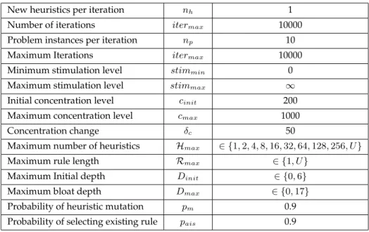
Parameters used in all experiments are given in table 3. These are unchanged from those used in previous works with additional parameters added relating to the initial and maximum depth for trees which are both set to either 0 or to 6 (dinit) and 17 (dmax)
respectively. The probabilitypaisandpmare set to high values to encourage
exploita-tion, i.e. mutation of existing rules and/or heuristics. This follows work reported in Sim and Hart (2014) that noted that the best results were obtained when new heuristics were formulated predominantly by mutating existing heuristics. Only two values of Rmax andDmaxwere investigated: Rmaxwas either set to 1 orU = unlimited, i.e. the
length of the sequence of rules defining a heuristics was either exactly one or set to unlimited, so that the sequences could grow to any length depending on the evolution-ary operators applied. The maximum depth of the trees was either set to 0 (use only a single terminal node) or 17 as in Koza (1992). The size of the ensemble was varied such thatH ∈ 1,2,4,8,16,32,64,128,256, U where U indicatesunlimited, i.e. no enforced restriction on the size of the ensemble.
As the rules are all stochastic (more than one operation may receive the highest priority score which results in a random selection from the set of highest priority oper-ations) all experiments were conducted 30 times, each for 10,000 iterations. This results in 30 sets of results for each training scenario: the heuristic(s) that gave the best results for each scenario during training were evaluated 30 times on set of 200 test problems using the corresponding objective function.
Table 3: Parameters
New heuristics per iteration nh 1
Number of iterations itermax 10000
Problem instances per iteration np 10
Maximum Iterations itermax 10000
Minimum stimulation level stimmin 0
Maximum stimulation level stimmax ∞
Initial concentration level cinit 200 Maximum concentration level cmax 1000
Concentration change δc 50
Maximum number of heuristics Hmax ∈ {1,2,4,8,16,32,64,128,256, U}
Maximum rule length Rmax ∈ {1, U}
Maximum Initial depth Dinit ∈ {0,6}
Maximum bloat depth Dmax ∈ {0,17}
Probability of heuristic mutation pm 0.9 Probability of selecting existing rule pais 0.9
68000 70000 72000 H1 D0 R1 H1 D0 RU H1 D17 R1 H1 D17 RU HU D0 R1 HU D0 RU HU D17 R1 HU D17 RU Total Summe d Makespan (a) 3.05 3.1 3.15 3.2 3.25 3.3 3.35 H1 D0 R1 H1 D0 RU H1 D17 R1 H1 D17 RU HU D0 R1 HU D0 RU HU D17 R1 HU D17 RU Total Summe d Weighte d Tardin ess (X 10 6) (b)
Figure 3: Results on the test problems for Makespan (left) and SWT (right)
5.1 Results
This section gives results from experiments in which ensembles were evolved using the training set of 500 instances and test set of 200 instances described in 4.4. Figure 3 shows boxplots that directly contrast performance when switching between trees, heuristics and ensembles on the test sets for both objectives. In each case, the four left-hand results (H=1) indicate ‘one-size-fits-all’ experiments in which a single heuristic is evolved. The right-hand four results represent ensembles, in which the components can consist of single rules (R=1) or sequences of rules (R=U). Configurations withDmax= 0
represent rules composed only of terminal nodes. Those withDmax= 17contain
tree-based rules. For theCmaxobjective,H1D0R1corresponds exactly to the rule−J RP T
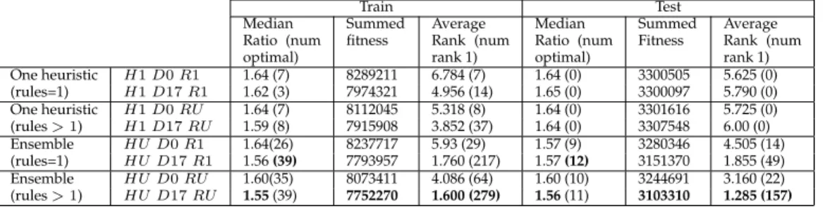
(annotated with conflict set B) shown in table 1 which is the best performing single terminal node and to−J ACT (again with conflict set B) for the SWT objective. The box plots present the summed fitness over the 200 test instances obtained from each configuration over 30 runs. The following general observations are made:
• Using an evolved rule (Dmax= 17) is always preferable to creating heuristics from
the terminal nodes only, regardless of whether ensembles or rule sequences are used
• For the non-ensemble methods (H=1), then a heuristic that contains a single rule rather than a sequence of rules is preferable: this is not observed in the ensemble methods in which the sequences (R=U) provide better results. This may result from overfitting on the training set when a single sequence is evolved, particularly forD= 0.
• Ensembles provide better results than a single ‘one-size-fits-all’ approach (H = 1), regardless ofRandD.
• The ensemble method used in conjunction withDU−RUis the clear winner, show-ing the benefit of an ensemble, of evolvshow-ing trees, and sequencshow-ing them into heuris-tics
Two-tailed t-tests between all pairs of results show that all observations are sta-tistically significant at the 5% confidence level, with the exception of the comparison
Table 4: CmaxFor each configuration<H*D*R*>, the table shows the median ratio to
theoretical optimal and summed fitness over all instances, and average rank compared to the other configurations. Results taken from the single best run in all cases.
Train Test Median Ratio (num optimal) Summed fitness Average Rank (num rank 1) Median Ratio (num optimal) Summed Fitness Average Rank (num rank 1) One heuristic H1D0R1 1.12 (4) 178329 7.452(4) 1.30 (1) 71236 6.355(2) (rules=1) H1D17R1 1.09 (62) 173299 4.486 (81) 1.10 (20) 69729 3.935(36) One heuristic H1D0RU 1.10 (78) 174113 4.232 (113) 1.15(0) 71914 6.945 (0) (rules>1) H1D17RU 1.09 (67) 172892 4.036 (90) 1.15 (0) 71286 6.415 (1) Ensemble HU D0R1 1.10 (49) 175151 5.474 (58) 1.10(19) 69970 4.225 (28) (rules=1) HU D17R1 1.05 (121) 169696 1.302 (363) 1.07 (40) 68146 1.405(129) Ensemble HU D0RU 1.07 (94) 171841 2.694 (191) 1.09 (25) 68976 2.555 (60) (rules>1) HU D17RU 1.05 (121 169777 1.400 (337) 1.07 (45) 68125 1.430(133)
H1D0R1toH1D17R1 using the SWT objective, where we were unable to find a sta-tistically better single rule that generalised better than the JATC rule, known for its performance on the SWT objective. However our results using ensembles (H > 1) improved on the single best rule on all occasions.
Tables 4 and 5 provide results from each configuration from the single best run obtained for both objectives. As the summed fitness metric used in figure 3 can be distorted by the larger instances, and masks performance on individual instances, we also provide an comparison to the theoretical optimal. For makespan this can be easily calculated (Taillard, 1993); the table gives the median value for the ratioactual/optimal makespan. For the TWT objective, we estimate thetheoretical optimal as the sum of the weighteddue-dates, and calculate the ratio of the summed weightedactualarrival date to the summed weighted due-dates. For both objectives, we also give the actual number of optimal solutions found. Additionally, we rank each of the 8 configurations on each instance (where rank 1 is best) and calculate the average rank over all instances, and the number of instances assigned rank 1 for each configuration.
In terms of the summed fitness, the ensemble composed of heuristics containing rule-sequences (HUD17RU) provides the best result for both objectives. Comparing average ranks and instances of rank 1, the same ensemble proves best for the TWT ob-jectives. It is marginally beaten by HUD17R1 for makespan in terms of average rank, but has more instances assigned rank 1. In terms of number of optimal solutions and median ratio, although the ensemble methods are clearly preferable, there is little differ-ence between the ensemble of rule sequdiffer-ences (HUD17RU) and the ensemble of single rules (HUD17R1). The RU configuration appears to faciliate the emergence of heuristics that improve fitness (reducing the sum) on some of the larger instances, while having little impact on the overall ratio to optimal, most likely due to the increased size of the search space.
5.2 Comparison to a Disposable Hyper-heuristic Approach
Hyper-heuristic methods aim to find quick and acceptable solutions to problems, often trading some loss in quality against speed of producing a solution. Given a new prob-lem instancepand a trained ensemble containinghheuristics, then exactlyhheuristics need to be executed once to find the best solution to the instance. In contrast, a typ-ical meta-heuristic approach applied to each instance to obtain a heuristic would run
Table 5:T W T For each configuration<H*D*R*>, the table shows the median ratio to theoretical optimal and summed fitness over all instances, and average rank compared to the other configurations. Results taken from the single best run in all cases.
Train Test Median Ratio (num optimal) Summed fitness Average Rank (num rank 1) Median Ratio (num optimal) Summed Fitness Average Rank (num rank 1) One heuristic H1D0R1 1.64 (7) 8289211 6.784 (7) 1.64 (0) 3300505 5.625 (0) (rules=1) H1D17R1 1.62 (3) 7974321 4.956 (14) 1.65 (0) 3300097 5.790 (0) One heuristic H1D0RU 1.64 (7) 8112045 5.318 (8) 1.64 (0) 3301616 5.725 (0) (rules>1) H1D17RU 1.59 (8) 7915908 3.852 (37) 1.64 (0) 3307548 6.00 (0) Ensemble HU D0R1 1.64(26) 8237717 5.93 (29) 1.57 (9) 3280346 4.505 (14) (rules=1) HU D17R1 1.56(39) 7793957 1.760 (217) 1.57(12) 3151370 1.855 (49) Ensemble HU D0RU 1.60(35) 8073411 4.086 (64) 1.60 (10) 3244691 3.160 (22) (rules>1) HU D17RU 1.55(39) 7752270 1.600 (279) 1.56(11) 3103310 1.285 (157)
fori iterations. Although not entirely fair, it is instructive to compare the quality of solutions obtained by greedy selection from an evolved ensemble to the quality of the solutions obtained by directly evolving a new heuristic to solve each individual in-stance. A standard GP algorithm with parameters set as in Koza (1992) (population size = 500, initialised using ramped half and half up to a depth of 6 using crossover 90% and cloning 10% and maximum tree depth of 17) was executed for 20 generations (10,000 evaluations as with NELLI-GP) is used. After initialisation, each tree is ran-domly assigned one of three possible rules to determine operation eligibility defined in section 3.1.2. This rule does not undergo mutation. The following experiments are performed 30 times:
• GP (1P) : GP is run on each of the 200 instances in the test set in isolation. i.e. a single rule is evolved for each test instance.
• GP (200P) : GP is run on the full set of the 200 test instances. i.e. 1 rule is evolved for the complete test set.
Table 6 shows the best, mean and standard deviation obtained over 30 runs. T-test results in each column show a comparison with the previous columns results. As well as results from the two experiments described, 3 sets of results from the exper-iments conducted in the previous section are included for comparison. GP (1P) and HU D17R1both evolves exactly one rule per problem, and hence can be directly com-pared. SimilarlyH1D17R1and GP (200P) both evolve a single rule that is evaluated on all 200 problem instances and hence are directly comparable. The results of apply-ing the best ensemble obtained durapply-ing trainapply-ing (H1 D17 RU) to the test set are also included.
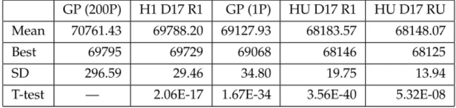
As would be expected GP(1P), which evolves a different rule for each problem in-stance, obtains better results than both GP(200P) andH1 D17 R1which evolve only a single generalist rule. Interestingly, when the evolved H1 D17 R1 rule is applied to the test set it outperforms the single rule that was evolved by GP directly on those instances, demonstrating good generalisation from the training set. All of the above re-sults are eclipsed by the rere-sults obtained by applying the reusableensemblesof heuris-tics generated by NELLI-GP. Furthermore the best trained ensemble (HU D17 RU), comprising of 264 heuristics, requires less than 3 % of the evaluations required for ei-ther of the GP experiments.
Table 6: Comparison of ensembles (Cmax)to disposable hyper-heuristic approaches
GP (200P) H1 D17 R1 GP (1P) HU D17 R1 HU D17 RU Mean 70761.43 69788.20 69127.93 68183.57 68148.07
Best 69795 69729 69068 68146 68125
SD 296.59 29.46 34.80 19.75 13.94
T-test — 2.06E-17 1.67E-34 3.56E-40 5.32E-08
5.3 Comparison to Existing Approaches
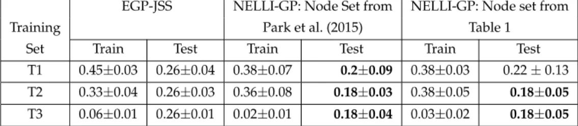
We compare our method to two recent approaches from the literature. Nguyen et al. (2013b) describe a new GP based approach to learning new iterative dispatching rules, using four well-known benchmarks datatsets (LA, ORB, TA, DMU). A training set is formed consisting of all odd numbered instances from each of the four sets, with the remainder making up a test-set. Each set has 105 instances. Park et al. (2015) use GP to evolve an ensemble of rules that vote to determine which operation is selected for scheduling at each iteration. Their approach is tested on the 80 instance Taillard (TA) set (which is included in Nguyen et al. (2013b)), using three different training sets each containing 5 instances, with the remaining 65 instances making up the test set in each case.
A direct comparison of ensemble methods is given by comparing NELLI-GP to the ensemble method of Park et al. (2015), i.e. the ‘Mixture-of-experts’ ensembles of the former and the majority voting approach taken by the latter. We use the same train-ing and test sets described in (Park et al., 2015) and evolve an ensemble of heuristics using NELLI-GP in the formH4 D17 RU in order to allow a fair comparison to the 4 islands used by Park et al. (2015). In order to provide an exact comparison, NELLI-GP is first limited to exactly the same set of function and terminal nodes used by Park et al. (2015). The experiment is then repeated using the full set of nodes given in table 7. Both NELLI-GP ensembles outperform the results from Park et al. (2015). T-tests at the 5% significance level confirm this result. T-tests additionally show no significant difference between the NELLI-GP results with different terminal sets. To compare to Nguyen et al. (2013b), we evolve an ensemble defined by HUD17RU using exactly the same training and test sets as their approach. Results averaged over 30 runs are given in the final line of table 8. NELLI-GP significantly outperforms the published approach on both training and test sets.
The ensembles evolved by NELLI-GP should be reusable. We take ensembles evolved on the new 500 training instances (as described in section 4.4) and reuse on the test sets used by Nguyen et al. (2013b) and Park et al. (2015), comparing to their published results. Results are given in table 8 for three ensembles (H4, H64, HU). All three significantly outperform EGP-JSS from Park et al. (2015) on the 65 Taillard in-stances. H8 and HU significantly outperform the results of the new GP method∆0
proposed by Nguyen et al. (2013b) and the results from their simple GP algorithm∆. Clearly the NELLI-GP ensembles arereusable— ensembles evolved on one data-set can be directly applied to adifferentdataset, and demonstrate improved performance over methods that were tailored to the tested dataset. In addition, the ensemble provides a robustoptimisation method. The instances in the datasets given in table 8 have similar parameters in terms of(jobs, machines)but contain operations whose processing times
Table 7: Comparison of NELLI-GP to EGP-JSS from Park et al. (2015) EGP-JSS NELLI-GP: Node Set from NELLI-GP: Node set from
Training Park et al. (2015) Table 1
Set Train Test Train Test Train Test
T1 0.45±0.03 0.26±0.04 0.38±0.07 0.2±0.09 0.38±0.03 0.22±0.13 T2 0.33±0.04 0.26±0.03 0.36±0.08 0.18±0.03 0.38±0.05 0.18±0.05 T3 0.06±0.01 0.26±0.01 0.02±0.01 0.18±0.04 0.03±0.02 0.18±0.05
Table 8: Reusability and robustness of ensembles: NELLI-GPT refers to ensembles
trained on the 500 new instances and applied directly to new test sets. Results from EGP-SS and∆,∆0taken directly from Park et al. (2015), Nguyen et al. (2013b) respec-tively. For comparison, NELLI-GPEgives the result from evolving an ensemble on the
same training set given in the relevant publications
Park et al. (2015) Nguyen et al. (2013b) 65 test instances 105 train 105 test (Park, 2015) EGP-JSS 0.26±0.001 (Nguyen, 2013) ∆ 0.179±0.003 0.187±0.005 ∆0 0.151±0.004 0.160±0.005 NELLI-GPT H4D17RU 0.18±0.005 0.178±0.001 0.171±0.002 H64D17RU 0.14±0.002 0.140±0.001 0.136±0.001 HU D17RU 0.15±0.002 0.140±0.001 0.136±0.001 NELLI-GPE HU D17RU 0.18±0.05 0.119±0.006 0.127±0.001
are drawn from different distributions to those used by the instances used to evolve the ensembles. Hence, they can be considered perturbed versions of the original instance set.
6
Analysis
This section provides an analysis of the ensemble in terms of the role and structure of the constituent heuristics, and relationship between heuristic performance and prob-lem structure.
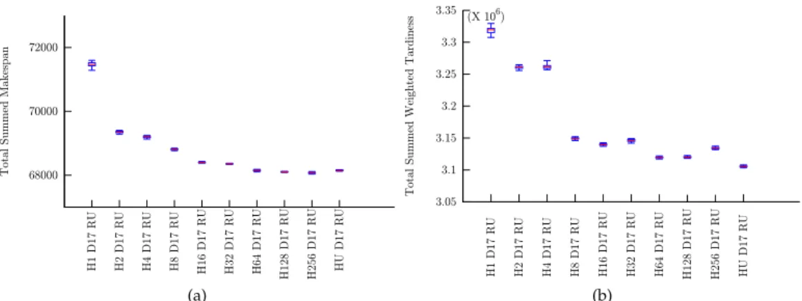
6.1 Effect of ensemble size
The experiments in section 5 allow ensembles of unlimited size (H = U) to evolve, although in practice evolution limits the actual size that emerges. In the following experiments, we examine the effect of restricting the size of the ensemble to H ∈ (1,2,4,8,16,32,64,128,256) rather than allowing evolution to proceed unrestricted. Figure 4 shows results on the test sets for both objective functions asHis varied.
A clear correlation between the size of the ensemble and the collective performance of the ensemble is apparent in all cases. However the benefit clearly tails off as the size of the ensemble increases beyond a saturation level. An ensemble size of|H| ≈ |P|/10
appears appropriate as a rule of thumb given the investigations conducted. However, this is clearly problem dependent, the larger and more diverse the training set the better the evolved heuristics.
68000 70000 72000 H1 D17 RU H2 D17 RU H4 D17 RU H8 D17 RU H16 D17 RU H32 D17 RU H64 D17 RU H128 D17 RU H256 D17 RU HU D17 RU Total Summe d Makespan (a) 3.05 3.1 3.15 3.2 3.25 3.3 3.35 H1 D17 RU H2 D17 RU H4 D17 RU H8 D17 RU H16 D17 RU H32 D17 RU H64 D17 RU H128 D17 RU H256 D17 RU HU D17 RU Total Summe d Weighte d Tardin ess (X 10 6) (b)
Figure 4: Varying ensemble size: Makespan (left) and SWT (right) results
6.2 Structure of evolved heuristics
The heuristics contained in evolved ensembles of size 1−264are analysed in terms of the number of rules contained in each heuristic, and the number of nodes in each rule, with results given in table 9. As previously noted the number of heuristics in the ensemble, the number of rules in a heuristic and the tree depth of the rules is an emergent property of NELLI-GP. Some general trends are observed. Heuristics tend to increase in complexity in terms of the number of rules-per-heuristic as the ensemble size increases, peaking at|H| = 64when the trend reverses. This suggests that large ensembles favour less complex rules, as each heuristic needs to operate in a smaller region of the instance space. In terms of nodes-per-rule, the pattern is less obvious; the number of nodes tends to increase as the size of the ensemble increases, but does not grow linearly. The average depth per rule is given in the final column — note that in all cases, this is significantly less that the maximum allowed depth of 17 and often produces small, easy to analyse heuristics with depth around 5. In contrast, in typical GP, bloat is common. We suggest that in NELLI-GP, bloat is largely suppressed by the elitist requirement that a heuristic must solve at least one instance better than the existing heuristics to replace another in the ensemble. In standard GP with a large population, weak trees can be sustained due to the replace-worst step, encouraging bloat. A typical rule taken from 1 of the heuristics from H64 R17 DU is shown in Figure 5
6.3 The role of the ensemble
To understand how each heuristic within the ensemble contributes to the collective performance we analyse an ensemble ofhheuristics applied to the set ofi= 200test instances. For each instance we calculatefi∗, i.e. the best result achieved on the instance by the ensemble, and calculatecias the number of heuristics that achievefi∗for a given
instancei.
For instances withci>1, multiple heuristics achieve the same resultf∗. From an
algorithmic perspective, we suggest that these instances do not represent ‘interesting’ regions in the instance space, given many heuristics perform equally well. In contrast,
Table 9: Analysis of the structure of the evolved heuristics
Actual H Avg R Avg Tnodes Avg Nodes Avg (max) Depth
per H per R per R Per R
H1D17RU 1 2 1 1 0 (0) H2D17RU 2 1.5 2.33 3.67 1.33 (2) H4D17RU 4 1 4.75 10 4.25 (5) H8D17RU 8 2.5 10.4 22.95 6.00 (7) H16D17RU 16 3.875 7.60 18.16 7.39 (12) H32D17RU 32 2.25 7.76 15.07 5.24 (9) H64D17RU 64 8.125 8.53 17.92 6.26 (10) H128D17RU 128 6.31 7.24 20.24 9.94 (12) H256D17RU 253 4.75 6.20 13.36 4.58 (9) HU D17RU 264 3.19 8.24 17.22 4.89 (8)
Figure 5: An average rule from 1 of the 64 heuristics evolved in experiment H64 R17 DU. The 64 heuristics contained on average 8 rules with rules having an average depth of 6. In general the depth of rules that emerged was much less than the maximum value of 17
H1 H2 H3 H4 H5 H6 H7 H8 Heuristic N umb er of in st an ce s w on 0 5 10 15 20 25 (a) Heuristic N umb er of in st an ce s w on 0 1 2 3 4 5 6 7 (b)
Figure 6: Number of instances uniquely won by each heuristic a) Ensemble of 8 heuris-tic (b) Ensemble of 64 heurisheuris-tics (sorted by wins)
ifci = 1, then the instance has a unique winner, and these instances represent regions
in which algorithm-selection becomes a key issue.
Letw(hj)be the number of instances won by heuristic,hj. Aspecialistheuristic, one
with smallw(hj), operates in a niche region of the instance space. Ageneralistheuristic
on the other hand, with largew(hj), operates across large regions of the space. The
balance between the specialist/generalist nature of the heuristics evolved is an emer-gent property of NELLI-GP that is closely linked to the structure of the instances in the dataset. We consider the 20 classes of makespan instances described in section 4.4 and the heuristics generated by the experimentH8D17RUandH64D17RU. Figure 6 shows the number of instancesw(hi)won by each of the heuristics for both experiments. For
an ensemble of 8 heuristics, we observe that for 32% of the 200 instances, there is no uniquely best heuristic. For the remaining 134 instances ‘interesting’ instances, no par-ticular heuristic is dominant; the most general heuristic (H3) wins 26 instances while the most specialist (H2) wins 11. In the ensemble of 64 heuristics, only 10% of instances do not have a unique winner. The 64 heuristics tend to specialise equally: the number of instances won ranges from 2-7, with no heuristic generalising across many instances.
6.3.1 Relationship between instance class and heuristic performance
NELLI-GP promotes the emergence of heuristics which are behaviourally diverse in that each heuristic has to uniquely win at least one instance in order to survive. As-suming that the instances within the subset won by each heuristic share similar fea-tures, we investigate theintra-class andinter-class membership of each subset, given the 20 classes defined in section 4.4. Figure 7 uses a network representation to cap-ture the relationships between heuristics and classes for an 8 heuristic ensemble. An edge exists between a heuristic and a class if the heuristic wins at least one instance in that class. The weight of the edge reflects how many instances within the class were won, and the size of a heuristic denotes how many different classes it wins instances in. The degree of aheuristicindicates the number of different classes the heuristic wins instances from. The degree of aclassindicates how many different heuristics win
in-H1 H2 H3 H4 H5 H6 H7 H8
Total processing time + + ++
Mean processing time ++ + ++
Processing time range ++ ++
Ratio jobs:machines ++ ++
Table 10: Examining the distribution of features in setIHi compared toIr, i.e. all re-maining instances. Table shows p-values obtained from Wilcoxon rank sum test for each feature
H1 H2 H3 H4 H5 H6 H7 H8
Total processing time ++ + +
Mean processing time
Processing time range + + + +
Ratio jobs:machines ++ ++
Table 11: Examining the distribution of features in setIHicompared toIu, i.e. the subset of remaining instances that are uniquely solved. Table shows p-values obtained from Wilcoxon rank sum test for each feature
stances from that class, thus is representative of intra-class niches. Heuristics have a median degree of 8.5, indicating there are clearly manyinter-class relationships be-tween instances. Classes have a median degree of 4, i.e. a typical class of 10 instances generated from the same parameter set has at least 4intra-class clusters. H3 is strongly associated with class 18 (defined by 25 jobs and 25 machines) winning 7/10 instances. Only 3 of the 20 classes are uniquely associated with a heuristic, implying uniformity across instances within these classes. Note that two of these classes (1,2) contain the easiest (in terms of finding optimal solutions) instances, due to the small number of jobs and machines.
Clusters of similar instances — those won by the same heuristic — naturally emerge from NELLI-GP. Each cluster can be examined with respect to a feature set to potentially identify correlations across instances. Ingimundardottir and Runarsson (2012) consider a set of 16 features and attempt to relate them to instance difficulty. 13 of these features are recalculated on a step-by-step basis after every operation has been scheduled (e.g. current makespan); the remaining 3 are static and apply to the instance as whole (e.g total job processing time). Smith-Miles et al. (2009) cluster instances (us-ing a tardiness objective) accord(us-ing to 6 features, then examine the distribution of fit-ness values to infer knowledge about the relationships between instance structure and heuristic performance. Taking the< H8>ensemble as an example, for each heuristic in turn we examine whether the features of the instances within the cluster defined by the instances it uniquely won differ significantly from the remainder of the instances. As NELLI-GP assigns a single heuristic to an instance, only static features are relevant. We consider four features: mean processing time, processing time range, total processing timeare used in both (Ingimundardottir and Runarsson, 2012; Smith-Miles et al., 2009); we addratio machines:jobsas this is known to influence problem hardness (Streeter and Smith, 2006).
If It is the 200 instances in the test set then let IHj be the subset of instances uniquely won by heuristicHj;Irthe subset ofallremaining instances fromIt;Iuthe
1 2 3 4 5 6 7 8 9 10 11 12 13 14 15 16 17 18 19 20 H1 H2 H3 H4 H5 H6 H7 H8
Figure 7: A network capturing the relationship between a heuristic the instance classes in which it wins instances. Edges are weighted according to the number of instances in the class won
instances inItuniquely won1by the remaining heuristics. For each of the four features,
we apply a Wilcoxon rank sum test to compare the feature values in the instances in IHi to those in subsetIr, and then separately to those inIu.
Results are shown in table 10 which differentiates between results significant at the 5% level (+) and at the 1% level (++). For three heuristics (H2, H5, H6) none of the features are discriminatory. However, for the remaining heuristics, at least one feature discriminates the instances won by the heuristic from the remainder of all in-stances or the remainder of heuristics uniquely won. All features are discriminatory in at least two tests. The results generally concur with the findings of Ingimundardottir and Runarsson (2012) who attempt to correlate features with hardness, noting that ‘the features distinguishing hard problems were scarce. Most likely due to their more complex data structure their key features are of a more composite nature’. NELLI-GP removes the need to define features in order to discriminate between instances; the clustering of instances emergesas a result of applying the algorithm. The emergent clusters capture structure within the problems that cannot be easily defined by humanly-intuitive features or by the features used togenerateinstances.
7
Conclusion
The automated design of reusable production scheduling heuristics is currently of great interest to the optimisation community as evidenced in detail by Branke et al. (2015). The need to move towardsensemble methods has been highlighted as an open chal-lenge, given the requirement to deal with complex decisions and varied problem in-stances. We have described a novel ensemble method for evolving JSSP heuristics called NELLI-GP in which each heuristic in the ensemble generates solutions to prob-lems in a niche region of the instance space.
Experiments on a large set of newly generated problem instances as well as exist-ing benchmarks have shown that novel rules can be evolved that outperform existexist-ing scheduling rules and recent hyper-heuristic methods. The power of the method is at-tributed to (a) evolving new dispatching rules that both define job-eligibility and use a large set of terminal; (b) Combining rules into variable length sequences to form new heuristics; (c) evolving ensembles of heuristics, in which each operates in a distinct part of the instance space. The reusability and robustness of the ensemble is demon-strated by applying an ensemble evolved on one set of instances to new instance sets, outperforming existing benchmarks. Analysing the evolved ensemble in terms of per-formance on different classes has enabled new insights to be gained relating to instance-structure. In agreement with Ingimundardottir and Runarsson (2012) we find that in-tuitive problem features are insufficient to characterise instances. Using the instance clusters that emerge from running NELLI-GP however, future work will focus on at-tempting to characterise the clusters in terms of combinations of known features or deriving new complex features. In addition, we intend to apply NELLI-GP todynamic scheduling problems in which it is possible to derive more fine-grained features.
Acknowledgment
This work is funded by EPSRC Grant Number EP/J021628/1
References
Applegate, D. and Cook, W. (1991). A computational study of the job-shop scheduling problem. ORSA Journal on Computing, 3(2):149–156.
Baker, K. R. (1984). Sequencing rules and due-date assignments in a job shop. Manage-ment Science, 30(9):1093–1104.
Bhowan, U., Johnston, M., Zhang, M., and Yao, X. (2013). Evolving diverse ensem-bles using genetic programming for classification with unbalanced data.Evolutionary Computation, IEEE Transactions on, 17(3):368–386.
Bhowan, U., Johnston, M., Zhang, M., and Yao, X. (2014). Reusing genetic programming for ensemble selection in classification of unbalanced data.Evolutionary Computation, IEEE Transactions on, 18(6):893–908.
Blackstone, J. H., Phillips, D. T., and Hogg, G. L. (1982). A state-of-the-art survey of dispatching rules for manufacturing job shop operations.International Journal of Pro-duction Research, 20(1):27–45.
Branke, J., Hildebrandt, T., and Scholz-Reiter, B. (2014). Hyper-heuristic evolution of dispatching rules: A comparison of rule representations. Evolutionary Computation, 23(2).
Branke, J., Nguyen, S., Pickardt, C., and Zhang, M. (2015). Automated design of pro-duction scheduling heuristics: a review. IEEE Transactions on Evolutionary Computa-tion.